Discovering Representative Models in Large Time Series Databases Simona Rombo DIMET Universit`a di Reggio Calabria Via Graziella, Localit`a Feo di Vito 89060 Reggio Calabria, Italy
[email protected]
Giorgio Terracina∗ Dipartimento di Matematica Universit`a della Calabria Via Pietro Bucci 87036 Rende (CS), Italy
[email protected] ∗ Corresponding author
Abstract The discovery of frequently occurring patterns in a time series could be important in several application contexts. As an example, the analysis of frequent patterns in biomedical observations could allow to perform diagnosis and/or prognosis. Moreover, the efficient discovery of frequent patterns may play an important role in several data mining tasks such as association rule discovery, clustering and classification. However, in order to identify interesting repetitions, it is necessary to allow errors in the matching patterns; in this context, it is difficult to select one pattern particularly suited to represent the set of similar ones, whereas modelling this set with a single model could be more effective. In this paper we present an approach for deriving representative models in a time series. Each model represents a set of similar patterns in the time series. The approach presents the following peculiarities: (i) it works on discretized time series but its complexity does not depend on the cardinality of the alphabet exploited for the discretization; (ii) derived models allow to express the distribution of the represented patterns; (iii) all interesting models are derived in a single scan of the time series. The paper reports the results of some experimental tests and compares the proposed approach with related ones. Keywords: Time Series, Frequent Pattern Discovery.
1
Introduction
In the literature, several approaches have been developed for efficiently locating previously defined patterns in a time series database (i.e., query by content) [1, 6, 9, 12, 13, 18]. However, a challenging issue is the discovery of previously unknown, frequently occurring patterns; indeed, in most cases, the patterns that could be of interest are unknown. As an example, some relevant medical problems are today faced by processing electrical signals detected on the human body; tests, such as the Electroencephalogram (EEG) or the Electrocardiogram (ECG) produce complex, large and analog signals allowing to perform diagnosis and/or prognosis. In this context, the discovery of frequently occurring patterns could be exploited to both identify disease-characterizing patterns and to foretell the risk of being subject to a disease. Some approaches have been already proposed in the literature for discovering frequent patterns [15, 17] or periodicities [4, 19] in time series. The knowledge discovery approaches for time series can be subdivided in two main categories: those ones working directly on the original time series and those ones requiring a discretized representation of them. Generally the former approaches are very precise 1
but more complex, since they require the application of complex mathematical operators, whereas the latter ones are more efficient but their precision and performance are constrained by the number of symbols (the alphabet) exploited in the discretization. A first contribution of this paper is the proposal of a technique exploiting a discrete representation of the time series but whose complexity does not depend on the size of the alphabet used for the discretization; this allows to preserve efficiency of discrete techniques yet maintaining a good accuracy of the results. The discovery of frequent patterns can play a relevant role both in the computation of time series similarities [2] and in several data mining tasks, such as association rule discovery [7, 11], clustering [8] and classification [14]. However, given a set of patterns characterized by a high similarity degree, it is difficult to select from them one representative pattern. This problem is even more relevant when the pattern must be exploited as a reference within different time series [2]. Some approaches exploit fitness measures [?] to select the most suited pattern; however, their effectiveness could be biased by the distribution of the patterns and the exploited fitness measure. A second contribution of this paper consists in the construction of models for frequent patterns appearing in a time series. Intuitively, a model is a pattern that may never be present in the time series which represents a set of patterns characterized by a high similarity degree. The construction of models provides two main benefits: • The recognition of characterizing features (i.e., representative patterns) from a time series is not biased by the relative differences among its patterns; indeed, approaches selecting one representative pattern from a set of similar ones need to determine the best pattern, among those in the set. On the contrary, the model generation phase is independent from the relative differences among the similar patterns. • Models simplify the comparison of characterizing features among different time series; this is important, for instance, in time series similarity detection approaches [2]. In this paper we carefully introduce the definition of model, we show the relationship between a model and the represented patterns and we present an algorithm for determining the K models best characterizing a time series. Finally, it is worth pointing out that the main problems arising in the discovery of frequent patterns in a time series are caused by both the length of the time series and the difficulty of efficiently computing the distance between the set of candidate frequent patterns and the portions of the time series. Indeed, a time series might contain up to billions of observations; as a consequence, minimizing the number of accesses to its values is mandatory. Moreover, the computation of distances between portions of the time series generally requires the construction of (possibly large) matrices and a number of comparisons which, in some cases, could be quadratic in the length of the time series [3, 16]. A third contribution of this paper consists in the definition of an approach which derives all interesting models in a single scan of the time series (thus minimizing the number of accesses to its values) and which exploits models to significantly simplify the identification of similar patterns. The plan of the paper is as follows: in Section 2 we provide some preliminary definitions and formally state the addressed problem. Section 3 describes the model extraction algorithm in detail whereas, Section 4 is devoted to present some results of experiments we have conducted on real data sets. In Section 5 we relate our proposal with existing ones pointing out similarities and differences among them; finally, in Section 6 we draw our conclusions.
2
2
Preliminaries
In this section we provide some preliminary definitions needed to describe our algorithm and we formally state the addressed problem. Definition 2.1 Time Series: A time series T = t1 , . . . , tm is a sequence of m values captured from the observation of a phenomenon. 2 Usually, time series regard very long observations containing up to billions of values. However, the main purpose of knowledge discovery on time series is to identify small portions of the time series characterizing it in some way. These portions are called subsequences. Definition 2.2 Subsequence: Given a time series T = t1 , . . . , tm a subsequence s of T is a sequence of l contiguous values of T , that is s = tq , . . . , tq+l , for 1 ≤ q ≤ m − l. 2 As we have pointed out in the Introduction, we require the input time series to be discretized. Our approach is quite independent from the discretization technique and any of the approaches already proposed in the literature (e.g., [6, 15, 13, 18]) can be exploited. Definition 2.3 Discretized Time Series: Given a time series T = t1 , . . . , tm and a finite alphabet Σ, the discretized time series D, obtained from T by applying a discretization function fΣ , can be represented as a sequence of symbols D = fΣ (T ) = α1 , . . . , αn such that αi ∈ Σ and n ≤ m. 2 Obviously, the accuracy of the discretization heavily depends on both the dimensionality reduction and the cardinality of Σ. As we will see in the following, the complexity of our approach does not depend on Σ; as a consequence, we may work on very accurate representations yet guaranteeing good performances. Analogously to what we have done for subsequences, we can introduce the concept of word. Definition 2.4 Word: Given a discretized time series D = α1 , . . . , αn , a word w of D is a sequence of l contiguous symbols in D, that is w = αq , . . . , αq+l , for 1 ≤ q ≤ n − l. 2 In this context, determining if two subsequences are similar, may correspond to determining if the associated words are equal. However, considering exact matches between words may produce too restrictive comparisons in presence of highly accurate discretizations. For this reason, we introduce the concept of distance between two words and of word similarity as follows. Definition 2.5 Distance: Given two words w1 and w2 , w1 is at an Hamming distance (or simply at distance) e from w2 if the minimum number of symbol substitutions required for transforming w1 in w2 is e. 2 Definition 2.6 Similarity: Given two words w1 and w2 and a maximum distance e, w1 and w2 are similar if the Hamming distance between them is less than or equal to e. 2 It is worth pointing out that the distance measure defined above is quite different from the Euclidean distance usually exploited for time series [6, 13, 18]; however, as we will show, this definition is one of the key features allowing our technique to have a complexity independent from the alphabet exploited in the discretization. In Section 3.2 we characterize the relationship between the distance defined above and the euclidean distance between two subsequences that are considered similar; moreover, in Section 4 we provide experimental results showing that this notion of distance allows to effectively identify sets of patterns sufficiently similar each other. 3
Example 2.1 Consider the words w1 = bcabb and w2 = baabc. By exploiting Definition 2.5 we say that w1 is at distance e = 2 from w2 . 2 Given a word w of length l, a time series may contain a set of up to Σei=1 (li )(|Σ| − 1)i distinct words at a distance less than or equal to e from w. However, none of them can be considered the most suited to represent this set. It is, therefore, necessary to refer to this set with one single word which is not present in the time series but correctly represents the whole set. We call this word a model for that set. In order to specify how models can be described, the following definition is important. Definition 2.7 Don’t care Symbol: Given an alphabet Σ, the “don’t care” symbol X is a symbol not present in Σ and matching, without error, all the symbols in Σ. 2 Example 2.2 Consider the words w1 = bcabb and w = baabc; both of them match exactly the word wM = bXabX. 2 Now, consider a generic word wM containing some don’t care symbols. This can be used to represent the set W SM of words in the time series exactly matching all the symbols of wM . As a consequence, we may say that wM represents or models W SM . Note that, for each pair of words wi , wj ∈ W SM , the maximum distance between wi and wj equals the number of don’t care symbols present in wM . Therefore, the number of don’t care symbols in a model can be exploited as the maximum distance considered acceptable for indicating that two words are similar. Finally, if we associate each don’t care symbol in the model with the list of symbols in Σ it must be substituted with for obtaining words in W SM , we are able to allow the model to express the distribution of the words in W SM . More formally: Definition 2.8 e-model: Given a discretized time series D and a maximum acceptable distance e, an e-model wM for D is a tuple of the form wM = hw, σ1 , . . . , σe i such that w ∈ {Σ ∪ X}+ is a word which contains e don’t care symbols and matches at least one word in D; each σi is a list of substitutions [ai1 |...|ais ] indicating the symbols that can be substituted to the ith don’t care symbol of w to obtain a word in D. 2 Example 2.3 Consider the discretized time series D=aabccdaddabbcadcaadbcad and a maximum distance e = 2. The tuple haXbcXd, [a|b|d], [a|c]i is an e-model for D; indeed, it represents the words {aabccd, abbcad, adbcad} in D. 2 When this is not confusing, we will represent the e-models in the more compact form aX[a|b|d]bcX[a|c]d or, simply, aXbcXd. Moreover, when it is not necessary to specify the number of don’t care symbols characterizing an e-model, we will use the terms e-model and model interchangeably. We are now able to formally state the problem addressed in this paper. Definition 2.9 Statement of the Problem: Given a discretized time series D, a maximum acceptable distance e and an integer K, our algorithm derives the K best e-models for D, that is the K e-models representing the maximum number of words in D. 2 Consider now a word w1 ; from Definition 2.8 we have that it can be modelled by (le ) different e-models, each one given by different positions of its e don’t care symbols. We call each of these models an e-neighbor of w1 , because it allows to represent a set of words at distance e from w1 . 4
Definition 2.10 e-neighbor set: Given a word w, the set of e-models representing it is called the e-neighbor set of w. 2 Example 2.4 Consider the word w = abcd and a maximum allowed distance e = 2. We have that the e-neighbor set of w is {abXX, aXcX, aXXd, XbcX, XbXd, XXcd} 2 Note that the e-neighbor set of a word w2 at distance e from w1 is only partially overlapped to the e-neighbor set of w1 . In this case, the overlapping models can be considered more representative than the other ones, since they represent more words. The following example illustrates this important concept. Example 2.5 Consider a distance e = 1 and the words w1 = aab and w2 = abb. The e-neighbor set of w1 is {aaX, aXb, Xab} whereas the e-neighbor set of w2 is {abX, aXb, Xbb}. Only the e-model aXb represents both w1 and w2 and, therefore, it is more representative than the other ones. The complete representation of this model is haXb, [a|b]i from which both w1 and w2 can be derived. 2
3
The Model Discovery Algorithm
The main idea underlying our approach is that of deriving the models during one single scan of the time series and minimizing the number of comparisons between candidate models. Indeed, the main problems arising in the discovery of frequent patterns in a time series are due to both the length of the time series and to the difficulty of efficiently computing the distance between the candidate patterns and the portions of the time series. As for the former problem, minimizing the number of accesses to the time series is important because this can contain up to billions of elements. As far as the latter one is concerned, classical approaches require the construction of (possibly large) matrices for the computation of distances and a number of comparisons which, in some cases, is O(n2 ) [3, 16]. In our approach, the role of models and, in particular, of don’t care symbols, is fundamental for solving both problems mentioned above. In particular, we scan the time series with a sliding window of length l and, for each extracted word we compute its e-neighbor set1 . Each e-model in the e-neighbor set is suitably stored and associated with a counter indicating the number of words it represents in the time series; each time a model is generated, its number of occurrences is incremented (the first time it occurs, its counter is set to 1). Moreover, when a model is stored, also the word it has been generated from is taken into account for updating its lists of substitutions (see Definition 2.8). At the end of the computation, only the K most frequent models are taken into account. From the description above, it should be clear that one important point in our approach is the efficient storage/update of the models. In order to solve this problem, we exploit a compact Keyword Tree [?] as support index structure for improving the efficiency of the algorithm. Keyword trees are tree-based structures which allow to efficiently store and access a set of words by representing their symbols as arc labels in the tree; each leaf node corresponds to the word that can be obtained by concatenating the symbols in the path from the root to that leaf node. The compact representation is obtained by collapsing chains of unary nodes into single arcs; words sharing the same prefixes share also the corresponding nodes and arcs in the tree. It is worth observing that: (i) if l is the length of the words stored in the tree, l is the maximum depth of the tree; (ii) the space required by a compact keyword tree is O(nw ), where nw is the number of distinct words it represents; this is motivated by the fact that, in the compact representation, each word insertion requires the creation of at most one 1
Recall that the e-neighbor set of a word is the set of e-models representing it.
5
Figure 1: Example of compact Keyword Tree storing a set of e-models internal node in the tree; (iii) common prefixes of different words share the same arcs, this allows sensible space savings; (iv) with the growing of the word lengths lower branches of the tree are mainly constituted by collapsed chains of unary nodes; in other words, this situation corresponds to an actual average depth of the tree lesser than l. Figure 1 illustrates an example of compact keyword tree storing a set of e-models of length 3 with e = 1. A pseudocode of our model discovery algorithm is given next: Input: A discretized time series D, and three integers l, e and K, representing, respectively, the length of the models to extract from D, the maximum distance considered acceptable and the number of best models to derive for D. Output: a set ResultSet containing the K best models for D. Type WordSet: Set of Words; var w, m: words; e-neighborSet, ResultSet: WordSet; T : Keyword Tree; pleaf : pointer; i,j : integer; begin ResultSet:= ∅; for i:=1 to Lenght(D) – l + 1 do begin w :=Subword(D,i,l); e-neighborSet:=Extract e-neighbors(w); for each m ∈ e-neighborSet do begin pleaf :=Insert(T,m,w); IncrementOccurrences(pleaf ); end; end; ResultSet:=FillResult(T,K); end;
Here, function Lenght receives a discretized time series D as input and yields as output its lenght. Function Subword receives a time series D and two integers i and l and returns the word of lenght l starting from position i in D. Function Extract e-neighbors derives the e-neighbor set of a word w. Obtained e-neighbors are stored in the set e-neighborSet. Function Insert receives a Keyword Tree T and two words m (representing a model) and w (representing the word the model has been derived from); it inserts m in T and returns the pointer to the leaf node of T associated with the last symbol of m. If m was not already present in T its 6
number of occurrences is set to 0. The function Insert exploits w to update the lists of substitutions associated with m; in particular, the symbol ai of w corresponding to the ith don’t care symbol of m is added to the list of substitutions σi associated with m. Function IncrementOccurrences receives a pointer pleaf and increments the number of occurrences stored in the node pointed by pleaf and corresponding to the last inserted model. Function FillResult receives a Keyword Tree T and an integer K as input and yields as output the set of K most representative models for D.
3.1
Complexity issues
As far as the computational complexity of our approach is concerned, the following considerations can be drawn. All the models are derived during one single scan of the time series; in particular, for each of the n symbols in the time series the following operations are carried out: l • The e-neighbors of the word of length l starting from that position are computed. ³ ´ These are (e ) and their construction, carried out by procedure Extract e-neighbor, costs O (le ) .
• Each e-neighbor is inserted in the keyword three and its number of occurrences is updated. In the worst case, the insertion of an e-neighbor is performed in O(l), whereas updating its number of occurrences can be performed in constant time. Finally, the last step of the computation is the selection of the best K models. Efficient implementations allow to perform this task in a time linear in the number of generated models which, in the worst case, is n(le ); note, however, that this number of models occurs only if all the generated models are different, which is mostly a theoretical case. ³ ´ Summarizing, the overall complexity of our algorithm is O nl(le ) . It is important to point out that: • Generally l