Discovering temporal patterns of differential gene expression in ...

Discovering temporal patterns of differential gene expression in microarray time series Oliver Stegle1 , Katherine J. Denby2 , Stuart McHattie2 , Andrew Mead2 , David L. Wild2 , Zoubin Ghahramani3 , Karsten M. Borgwardt1 1 Max Planck Institutes T¨ubingen, 2 University of Warwick, 3 University of Cambridge Abstract: A wealth of time series of microarray measurements have become available over recent years. Several two-sample tests for detecting differential gene expression in these time series have been defined, but they can only answer the question whether a gene is differentially expressed across the whole time series, not in which intervals it is differentially expressed. In this article, we propose a Gaussian process based approach for studying these dynamics of differential gene expression. In experiments on Arabidopsis thaliana gene expression levels, our novel technique helps us to uncover that the family of WRKY transcription factors appears to be involved in the early response to infection by a fungal pathogen.

1

Introduction

Microarray data are a major resource for studying the response of an organism to external conditions and stimuli. In the past, the majority of studies considered only a single measurement in each condition. Recent advances in microarray technology and falling costs have led to an increasing number of studies where expression levels are measured in different conditions over time rather than in a single snapshot. A range of techniques to test for differential expression have been proposed in the computational biology and statistics communities. In statistics, this task is often referred to as the two-sample problem. The majority of these existing methods are aimed at identifying differentially expressed genes from static microarray experiments, for example (KMC00, DYCS02, ETST01). More recent approaches are specifically designed for time series (JGS+ 03; SXL+ 05; TS06; CDCMP07; ACC+ 08), and a range of desired properties of a two-sample test for microarray time series have been established. First, the test should explicitly address the dependencies between consecutive measurements. Second, the method should not make overly strong assumptions about functions describing the time series, such as assuming a linear or finite model basis (Yua06). Third, to accommodate data characteristics specific to the microarray platform, it is beneficial to handle missing values and deal with multiple replicates. Finally, robustness with respect to outliers has proven useful for reliable results on microarray datasets (CDCMP07; ACC+ 08). To address all of these issues, we defined a robust Bayesian two-sample test for differential gene expression using Gaussian processes (GP) in (SDW+ 09). In addition to solving the basic two-sample problem, the presented method can also be used to decide whether

differential expression occurs at a specific time point in the time series. However, the test from (SDW+ 09) does not reflect‘smoothness’ between decisions at consecutive time points. That is, there can be abrupt switches from non-differential gene expression to differential gene expression (and vice versa) from one time point to the next. If one wants to detect meaningful temporal intervals of differential gene expression rather than individual time steps, it is vital to incorporate this smoothness assumption into the formulation of the statistical model. This is exactly the goal of this article. The remainder of this article is organised as follows. We start by reviewing how Gaussian processes can be applied to test for differential expression in microarray time series (SDW+ 09). In Section 3, this basic test is extended to a temporal model detecting intervals of differential gene expression. Finally, in Section 4, we demonstrate how this additional information can be useful to gain insights into regulatory mechanisms involved in the response of Arabidopsis to an infection by a fungal pathogen.

2

Gaussian Process-based two-sample test

The task of detecting differential gene expression is defined as follows: Given observed gene expression levels from two biological replicates that are exposed to different conditions, the goal is to determine whether a given gene probe is differentially expressed in these conditions or not. The principle underlying the Gaussian process-based two-sample test (GPTwoSample) from (SDW+ 09) is the comparison of two models: The first model assumes that the microarray time series in both conditions are samples drawn from an identical shared distribution. An alternative model describes the time series in both conditions as samples from two independent distributions. As these distributions need to be defined over functions, a Gaussian process is an appealing model. A GP incorporates beliefs about smoothness and allows all model parameters except for a handful of hyperparameters to be integrated out analytically, allowing for tractable model comparison. The two alternatives, the shared model (HS ) and the independent model (HI ) can then be objectively compared using the logarithm of the Bayes factor Score = log

P (DA , DB | HI ) , P (DA , DB | HS )

(1)

where DA and DB are observed expression levels in two conditions A and B. Writing out the GP models explicitly leads to Score = log

P (YA | HGP , TA , θ I )P (YB | HGP , TB , θ I ) , P (YA ∪ YB | HGP , TA ∪ TB , θ S )

(2)

where Y A/B are observed expression levels and T A/B are the corresponding time points in both conditions and θ I , θ S are hyperparameters of both models. For details see (SDW+ 09).

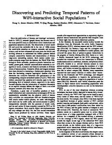
Figure 1: Bayesian network for the temporal GPTwoSample model. At observed time points {tn }, binary indicator variables {ztn } determine the state of a gate and hence which expert explains the corresponding observations. If the state of the indicator is 1 the independent expert is used, while if the switch is 0, the shared expert is used. The shared expert uses a single GP f (t) to model both conditions. The independent expert uses two GPs f A (t), f B (t). Smoothness of the GP priors is indicated by the thick bands coupling function values at different time points. A logistic Gaussian process, g(t), incorporates smoothness over the state of the indicator variables.

3

Detecting intervals of differential gene expression

Once we know that a particular gene is differentially expressed, it is interesting to ask in which intervals of the time series this effect is present. Such detailed analysis is particularly valuable for longer time series, where differential behaviour might be present only temporarily or occur after a certain time delay. To address this question, we propose a mixture model over time, where one mixture component (expert) corresponds to the shared model and a second mixture component to the independent model. A Bayesian network representation of this temporal GPTwoSample model is shown in Figure 1. The model is closely related to mixtures of Gaussian process experts (RG01). The shared expert is a single GP explaining expression levels in both conditions, while the independent expert uses a separate GP for each condition. At observed time points binary switches z = {zt1 , . . . , ztn } determine which expert explains the corresponding expression levels. In the same way that the expression levels vary smoothly over time, we also believe that the states of the indicators follow a smooth trend, typically reflecting a transition from the shared expert to the independent expert. This belief about smoothness is expressed in a gating network, implying a joint probability

distribution over all indicators P (z | T, θ G ). The coupling of the observed expression levels Y by the GP experts renders inference in this mixture model difficult. While the latent function values f can be integrated out in closed form, marginalising over the state of the indicators z yields an exponential sum over all possible configurations: X  P (Y | T, θ S , θ I , θ G ) = P (z | θ G ) P (Y{yn :ztn =0} | HS , T{tn :ztn =0} , θ S ) z

 ×P (Y{yn :ztn =1} | HI , T{tn :ztn =1} , θ I ) .

(3)

The two terms in the sum are the data likelihoods from both GP experts introduced in Section 2. Here we follow (RG01) and exploit tractable conditional distributions. Conditioned on a particular configuration of the indicators z, the likelihood factorises into a product over the two experts, where the data are split between the experts according to the state of the indicator variables. A Gibbs sampler is well suited for this inference task. The latent function values of the experts can be integrated out or collapsed and hence Gibbs sampling steps reduce to updates of one indicator at a time, conditioning on the current state of all remaining indicators and data. The conditional distribution over a particular indicator zti is     P zti = s | z\ti , T, Y, θ S , θ I , θ G ∝P Y | zti = s, z\ti , T, θ I , θ S   ×P zti = s | z\ti , θ G , (4) with s ∈ {0, 1}. The first term is the conditional data likelihood. Rewriting this term as   P Y | zti = s, z\ti , T, θ I , θ S =P (yti | zti = s, z\ti , Y\yti , T) ×P (Y\yi | z\ti , T\ti )

(5)

reveals that for Gibbs sampling it is sufficient to calculate the probability of yti under the leave-one-out predictive distribution of both GP experts. The second term in (4) is the probability of the indicator zti under the predictive distribution of the gating network, given all other indicators. We choose a logistic Gaussian process as a gating network, where smoothness is expressed by a GP prior on a latent function g(t) (Figure 1). Bernoulli predictions of an indicator zti are related to the Gaussian predictive function values by a probit likelihood model (full details in accompanying technical report), Z
\ti P (zti = 1 | z , T) = Φ(gti )N gti µti , σt2i dgti . (6) g ti

The likelihood models of both Gaussian process experts as well as the gating network are all non-Gaussian and hence predictive distributions are not available in closed form. Expectation Propagation (EP) (see tech report, (SDW+ 09)) is applied to all these cases to obtain tractable approximate predictive densities.

Sampling of the indicators is repeated for a number of randomised sweeps through all indicators. After every full sweep, the GP hyperparameters from the GP experts and the gating function are sampled using Hamiltonian Monte Carlo (e.g. (Mac03)). The complete sampling scheme is summarized in Algorithm 1. Algorithm 1 Sampling scheme for the temporal GPTwoSample model for ng = 1 . . . Ng Gibbs sweeps do for n ∈ 1, . . . , N measurements do Resample indicator ztn (Equation (4)). end for Sample the hyperparameters θ S , θ I and θ G conditioned on z. 6: end for 1: 2: 3: 4: 5:

To identify temporal patterns of differential expression, we are most interested in the inferred states of the indicators. After a burn-in period, the generated samples yield an empirical posterior distribution over the indicator variables z. Predictions of the gating network at test times t? can be obtained by integrating out z using a set of S samples P (z? = 1 | Y, T, t? ) ≈

S 1X (s) P (z? = 1 | Y, T, t? , z(s) , θ G ), S s=1

(7)

yielding a mixture of Bernoulli distributions. These marginal predictions ignore the coupling at different time points that is introduced from the sampled states {z(s) }. However, after a sufficient burn-in period, most of the indicators are constant across samples {z(s) } and hence marginal predictions are appropriate. The same argument applies to predictions of the latent function values of the GP experts. These mixtures of Gaussians are well approximated by a Gaussian predictive distribution.

4

Detecting transition points in Arabidopsis microarray time series

We applied the temporal GPTwoSample model1 to detect intervals of differential expression of gene probes from an Arabidopsis time series dataset. In this particular experiment, the stress response of interest is an infection of Arabidopsis thaliana by the fungal pathogen Botrytis cinerea. The ultimate goal is to elucidate the gene regulatory networks controlling the plant defense against this pathogen. The identification of intervals of differentially expressed genes is an important first step towards this goal. Data were obtained from an experiment in which detached Arabidopsis leaves were inoculated with a B. cinerea spore suspension (or mock-inoculated) and harvested every 2 hr up to 48 hr post-inoculation for a total of 24 time points. B. cinerea spores (suspended in halfstrength grape juice) germinate, penetrate the leaf and cause expanding necrotic lesions. Mock-inoculated leaves were treated with droplets of half-strength grape juice. At each time point and for both treatments, one leaf was harvested from four plants under identical 1 Software

will be made available with the accompanying tech report.

Figure 2: An example result produced by the GPTwoSample temporal test. Top: The posterior probability of differential expression as a function of time. Bottom: Dashed lines represent replicates of gene expression measurements for control (green) and treatment (red). Thick solid lines are Gaussian process mean predictions of the latent process traces; error bars of plus or minus 2 standard deviations are indicated by shaded areas. The intensity of the shaded areas is modulated by the posterior probability of the respective Gaussian process expert. The score in the figure title is the Bayes factor of the standard GPTwoSample test. conditions (i.e. there were 4 biological replicates). Full genome expression profiles were generated from these whole leaves covering a total of 30,336 gene probes. In the experiments, we used our novel test for detecting intervals of differential gene expression for each of the 30,336 probes. In the computations, a total of 50 Gibbs sweeps were performed. After every Gibbs sweep 5 Hamiltonian Monte Carlo updates were interleaved. To allow for a burn-in period, posterior parameters were estimated from samples of the last 25 sweeps. Figure 2 gives an example result of the temporal GPTwoSample model. The top panel shows the marginal predictive distribution for the indicator state z(t), choosing between the shared, z(t) = 0, and the independent, z(t) = 1, expert. The bottom panel shows the raw data and marginal predictions of latent function values from both GP experts. For this particular gene the test identified intervals of clear differential expression that started at around 22 hr post inoculation and lasted until the end of the time series recording. Additional results for a representative selection of gene probes are shown in Figure 3. Delayed differential expression Applying the temporal GPTwoSample test to a large set of differentially expressed genes, it is possible to study the distribution of their start and stop times of differential expression.

(a) CATMA1a64350: Early diff. expr.

(b) CATMA2c47710: Delayed diff. expr.

(c) CATMA1c71184: Transient diff. expr.

(d) CATMA5a14990: Permanent diff. expr.

Figure 3: Example results of the temporal GPTwoSample model applied to the Arabidopsis data. Panels (a) and (b) show examples of particularly early and late differential expression. In (c) a gene probe is shown for which differential expression appeared to be transient. Example (d) shows a probe with weak evidence for differential expression throughout the time series. For this analysis, the top 6000 genes that had a score suggesting significant differential expression were used. For each gene the start time of differential expression was determined as the first time point at which the posterior probability of differential expression, P (ztn = 1), exceeded 0.5, evaluated at a discretisation of 100 points in the interval [0, 50] hr. Analogously the stop time was deduced as the time point where differential expression ended, i.e. P (ztn = 0) ≤ 0.5. The lower panel in Figure 4 shows the histogram of the start time for the considered 6000 gene probes. The identification of transition points for individual gene expression profiles shows that a significant change in the transcriptional program began at around 17 hr post-inoculation. This program of gene expression change appeared to have two strong waves peaking around 21 hr and 25 hr. For a small fraction of genes this change in the transcriptional program started at either significantly earlier or later times; Figures 3a and 3b give examples of such genes. Figure 3d shows results for one of the approximately 200 genes that were identified as differentially expressed right from the start of the time series. Most of these genes were weakly expressed and an offset between the measurements in both conditions triggered the early classification as differentially expressed. The top panel of Figure 4 shows the stop time of differential expression for 13 genes for

Figure 4: Histogram of the most likely start and stop of differential expression for the top 6000 differentially expressed genes. Stop time are shown for a total of 13 genes that appear to exhibit transient differential expression ending within the observed time window. which the differential expression program ended within the measured time interval. An example of one of these genes with transient differential expression is given in Figure 3c. Interpreting waves of differential expression It is interesting to understand the causes for the different onset-timings of differential expression for individual genes. We expect regulators (if involved in the response to the fungus infection) to be expressed at earlier times than the downstream genes they control. In the Arabidopsis response to stress, several relevant regulatory mechanisms have been established in the literature. These include transcription factors (CPG+ 02; SYS00) as well as kinases (FFN+ 06; CRBX05). Figure 5 shows histograms of the start time of differential expression for groupings of the 6000 genes that correspond to different gene categories. Tentatively, transcription factors and kinases appeared to be stronger represented in the earlier wave; however application of a Kolmogorov-Smirnov (KS) test revealed that these differences were not significant (transcription factors: p = 0.092, kinases: p = 0.964). The differential expression onset-timing can be broken down further, for instance into subfamilies of transcription factors. The family of WRKY transcription factors is known to play a role in response to biotic stresses (CPG+ 02). The onset times of transcription factors in this family appeared to be overrepresented in early differential expression compared to other transcription factors. A KS-test revealed that this subset of 26 transcription factors exhibited a significantly different distribution of onset-times than other genes (p = 3.3 · 10−6 ). This results demonstrates the usefulness of the time-local two-sample test. By analysing the onset timing it is possible to narrow down the set of interesting candidate genes to study. When designing further experiments to elucidate transcriptional networks mediating the defense response against B. cinerea, regulatory genes whose expression first changes in the 21 hr wave or earlier would be of particular interest.

Figure 5: Histogram of the most likely start differential expression for the top 6000 differentially expressed genes split up into different gene categories. From top to bottom the histograms show results for all 6000 genes, kinases , known and putative transcription factors and WRKY transcription factors.

5

Discussion and outlook

The temporal GPTwoSample model, which we presented in this article, extends the standard paradigm of the two-sample problem and our previous work (SDW+ 09) to the identification of smooth intervals of differential expression. The proposed method is computationally efficient and can be applied to large datasets with thousands of genes using a standard desktop PC. Experimental results on 6000 differentially expressed Arabidopsis thaliana gene probes revealed patterns in the timing of the response to a fungal infection (Figure 3). As an example application we studied the distribution of the start and stop times of differential expression (Figure 4) that led to insights on waves of differential expression in Arabidopsis genes (Figure 5). Several extensions of the method developed in this article would be of interest. First, the current model does not distinguish between different expression patterns and anti correlated genes. Explicit modeling of anti-correlation is an important next step. Second, extensions to model differential gene expression at a network view rather than at the level of individual genes are an interesting direction of future development of differential gene expression models. The presented method provides the required per-gene level model for such future investigation.

References [ACC+ 08] C. Angelini, L. Cutillo, D. Canditiis, M. Mutarelli, and M. Pensky. BATS: a Bayesian user-friendly software for Analyzing Time Series microarray experiments. BMC Bioinformatics, 9(1):415, 2008. [CDCMP07] Angelini C., D. De Canditiis, M. Mutarelli, and M. Pensky. A Bayesian Approach to

Estimation and Testing in Time-course Microarray Experiments. Statistical Applications in Genetics and Molecular Biology, 6, September 2007. [CPG+ 02] W. Chen, N.J. Provart, J. Glazebrook, F. Katagiri, H.S. Chang, T. Eulgem, F. Mauch, S. Luan, G. Zou, S.A. Whitham, et al. Expression profile matrix of Arabidopsis transcription factor genes suggests their putative functions in response to environmental stresses. The Plant Cell Online, 14(3):559, 2002. [CRBX05] M. Cvetkovska, C. Rampitsch, N. Bykova, and T. Xing. Genomic analysis of MAP kinase cascades in Arabidopsis defense responses. Plant Molecular Biology Reporter, 23(4):331–343, 2005. [DYCS02] S. Dudoit, Y. H. Yang, M. J. Callow, and T. P. Speed. Statistical methods for identifying differentially expressed genes in replicated cDNA microarray experiments. Statistica Sinica, 12:111–140, 2002. [ETST01] B. Efron, R. Tibshirani, J. D. Storey, and V. Tusher. Empirical Bayes Analysis of a Microarray Experiment. Journal of the American Statistical Association, 96:1151– 1160, 2001. [FFN+ 06] M. Fujita, Y. Fujita, Y. Noutoshi, F. Takahashi, Y. Narusaka, K. Yamaguchi-Shinozaki, and K. Shinozaki. Crosstalk between abiotic and biotic stress responses: a current view from the points of convergence in the stress signaling networks. Current Opinion in Plant Biology, 9:436–442, August 2006. [JGS+ 03] Z.V. Joseph, G. Gerber, I. Simon, D.K. Gifford, and T.S. Jaakkola. Comparing the continuous representation of time-series expression profiles to identify differentially expressed genes. Proceedings of the National Academy of Sciences of the United States of America, 100:10146–51, September 2003. [KMC00] M.K. Kerr, M. Martin, and G.A. Churchill. Analysis of Variance for Gene Expression Microarray Data. Journal of Computational Biology, 7(6):819–837, 2000. [Mac03] D. J. C. MacKay. Information Theory, Inference, and Learning Algorithms. Cambridge University Press, 2003. [RG01] C. E. Rasmussen and Z. Ghahramani. Infinite Mixtures of Gaussian Process Experts. In Advances in Neural Information Processing Systems, volume 13, pages 881–888. MIT Press, 2001. [SDW+ 09] O. Stegle, K. Denby, D. L. Wild, Z. Ghahramani, and K. M. Borgwardt. A robust Bayesian two-sample test for detecting intervals of differential gene expression in microarray time series. Lecture Notes in Computer Science (RECOMB), 2009. [SXL+ 05] J. D. Storey, W. Xiao, J. T. Leek, R. G. Tompkins, and R. W. Davis. Significance analysis of time course microarray experiments. Proceedings of the National Academy of Sciences of the United States of America, 102:12837–42, September 2005. [SYS00] K. Shinozaki and K. Yamaguchi-Shinozaki. Molecular responses to dehydration and low temperature: differences and cross-talk between two stress signaling pathways. Current Opinion in Plant Biology, 3(3):217–223, 2000. [TS06] Y. C. Tai and T. P. Speed. A multivariate empirical Bayes statistic for replicated microarray time course data. Annals of Statistics, 34:2387–2412, 2006. [Yua06] M. Yuan. Flexible temporal expression profile modelling using the Gaussian process. Computational Statistics and Data Analysis, 51:1754–1764, 2006.