Discovery and Application of Functional ... - Semantic Scholar

Discovery and Application of Functional Dependencies in Conjunctive Query Mining Bart Goethals1 , Dominique Laurent2 , Wim Le Page1 1

University of Antwerp, Dept of Mathematics and Computer Science B-2020 Antwerp 2 ETIS-CNRS-ENSEA-Universit´e de Cergy-Pontoise F-95000 Cergy-Pontoise

Abstract. We present an algorithm for mining frequent queries in arbitrary relational databases, over which functional dependencies are assumed. Building upon previous results, we restrict to the simple, but appealing subclass of simple conjunctive queries. The proposed algorithm makes use of the functional dependencies of the database to optimise the generation of queries and prune redundant queries. Furthermore, our algorithm is capable of detecting previously unknown functional dependencies that hold on the database relations as well as on joins of relations. These detected dependencies are subsequently used to prune redundant queries. We propose an efficient database-oriented implementation of our algorithm using SQL, and provide several promising experimental results.

1

Introduction

The discovery of recurring patterns in databases is one of the main topics in data mining and many efficient solutions have been developed for different classes of patterns and data collections. Almost all techniques, however, work on so called transaction databases [1]. Not only for itemsets, but also in the case of trees [20] and graphs [12, 15, 19], the database consists of a collection of transactions, and a frequent pattern is discovered if it occurs in enough such transactions. Even in the multi-relational case, as considered in the WARMR system [4], the database can be seen as a collection of transactions in which each transaction consists of a small relational database. A query is then called frequent if it gives a non-empty answer in enough of such databases. Obviously, many relational databases are not suited to be converted into such a transactional format and even if this would be possible, a lot of information implicitly encoded in the relational model would be lost after conversion. Recently, we have considered association rule mining on arbitrary relational databases by combining pairs of queries which could reveal interesting properties in the database [8, 13]. Intuitively, we pose two queries on the database such that one query is more specific than the other (w.r.t. query containment). Then, if the number of tuples in the output of both queries is almost the same, a potentially interesting discovery is revealed. To illustrate, consider the well known Internet Movie Database [11] containing almost all possible information about movies, actors and everything related to that, and consider the following queries: first, we ask for all actors that have starred in a movie of the genre ‘drama’; then, we ask for all actors that have starred in a movie of the genre ‘drama’, but that also starred in a (possibly different) movie of the genre ‘comedy’.

2

Now suppose the answer to the first query consists of 1000 actors, and the answer to the second query consists of 900 actors. Obviously, these answers do not necessarily reveal any significant insights on themselves, but when combined, it reveals the potentially interesting pattern that actors starring in ‘drama’ movies typically (with a probability of 90%) also star in a ‘comedy’ movie. Of course, this pattern could also have been found by first preprocessing the database, and creating a transaction for each actor containing the set of all genres of movies he or she appeared in. Similarly, a pattern like: 77% of the movies starring Ben Affleck, also star Matt Damon, could be found by posing the query asking for all movies starring Ben Affleck, and the query asking for all movies starring both Ben Affleck and Matt Damon. Again, this could also be found using frequent set mining methods, but this time, the database should have been differently preprocessed in order to find this pattern. Furthermore, it is even impossible to preprocess the database only once in such a way that the above two patterns would be found by frequent set mining, as they are counting different types of transactions: actors in the first example and movies in the second example. Also truly relational patterns can be found which can not be found using typical set mining techniques, such as 80% of all movie directors that have ever been an actor in some movie, also star in at least one of the movies they directed. This is expressed by two queries of which one asks for all movie directors that have ever acted, and the second one asks for all movie directors that have ever acted in one of their own movies. The Conqueror algorithm recently developed by Goethals et al. [8] has shown to discover interesting association rules over a simple, but appealing subclass of conjunctive queries, called simple conjunctive queries. Furthermore, the algorithm had an efficient database-oriented implementation in SQL. One challenge that remained to be solved in this approach, was the huge number of generated patterns. Part of the volume is inherently due to the relational setting, but a substantial part, however, is due to redundancies induced by dependencies embedded in the data. Jen et al. [13], studied the problem of mining all frequent queries from a single relational table. They considered projection-selection queries, and assumed that the table to be mined satisfies a set of functional dependencies. A pre-ordering over queries was defined, and shown to be anti-monotonic towards the support measure. Moreover, this pre-ordering induces an equivalence relation and two equivalent queries are shown to have the same support. Therefore, one computation per equivalence class allows to know the support of all queries in that class. In [14], this work has been generalised to several tables in the case where the database operates over a star schema. The challenge however remains to generalise the theory to arbitrary relational databases. Clearly, the combination of the approaches in [13] and [8] would resolve the issues posed, i.e., mining non redundant simple conjunctive queries (thus including arbitrary joins), given a collection of functional dependencies over the relations of an arbitrary relational database. This is one major contribution of this paper. Moreover, combining these techniques also results in new opportunities. That is, next to the given functional dependencies, we introduce a novel technique to discover previously unknown functional dependencies, and immediately exploit them for reducing the number of frequent queries in the output. Furthermore, we do so not only for the relations of the database, but also for any join of relations. This is the second con-

3

tribution of this paper, and several experiments clearly show the benefits of this approach, thus making the discovery of simple conjunctive queries a feasible and attractive method towards the exploration of arbitrary relational databases. The paper is organised as follows: In Section 2, we recall the basic concepts and definitions used in this work and we briefly review from [13] how functional dependencies are used to compare queries. We present our algorithm Conqueror+ in Section 3, combining the two approaches [8, 13], and in Section 4, we report experiments, showing that Conqueror+ clearly outperforms Conqueror. We conclude in Section 6.

2 2.1

Formal Model Background

We consider a fixed attribute set U and a relational database schema D = {R1 , . . . , Rn } over U in which, for i = 1, . . . , n, Ri is a relation name associated with a subset of U , called the schema of Ri and denoted by sch(Ri ). Without loss of generality, we assume that, for all distinct i and j in {1, . . . , n}, sch(Ri ) ∩ sch(Rj ) = ∅. In order to make this assumption explicit, for all i in {1, . . . , n}, every A in sch(Ri ) is referred to as Ri .A. We also assume that we are given functional dependencies over D. More precisely, each Ri is associated with a set of functional dependencies over sch(Ri ), denoted by FDi , and the set of all functional dependencies defined in D is denoted by FD. As in [8], the queries of interest in our approach, are conjunctive projection-selectionjoin queries whose joins are expressed using a conjunction of selection conditions of the form Ri .A = Rj .A0 . We note that by doing so, all possible equi-joins can be considered, which would not the case using the universal relation associated to the given database. Moreover, we recall from [8] that such a conjunctive condition F induces a partition blocks(F ) of U , where every block β of blocks(F ) is a maximal set of attributes such that for all Ri .A and Rj .A0 in β, Ri .A = Rj .A0 is a consequence of F . In such a case, we say that Ri and Rj are connected through F . Definition 1 Denoting by R the cartesian product R1 × . . . × Rn , let Q = πX σF R where F = o n(Q) ∧ σ(Q), such that o n(Q) and σ(Q) are respectively conjunctions of selection conditions of the form Ri .A = Rj .A0 and Rk .A = a, where i, j and k are in {1, . . . , n} and a is in dom(A). Q = πX σF R is said to be a simple conjunctive query if all relation names occurring in X or in σ(Q) are connected through o n(Q). Given a simple conjunctive query Q = πX σF R, the set X is denoted by π(Q) and the tuple defined by the conjunctive selection condition σ(Q) is denoted by Qσ . We call Q a join query if σ(Q) is the empty condition and if π(Q) is the set of all attributes of all relation names occurring in o n(Q). Given a simple conjunctive query Q, we denote by J(Q) the join query such that o n(J(Q)) =o n(Q). To simplify notation, given a simple conjunctive query Q, the corresponding partition of U , blocks(o n(Q)) is simply denoted by blocks(Q). We emphasise that, according to Definition 1, considering simple conjunctive queries avoids computing cartesian products. We illustrate this definition below.

4

Example 1. Let us consider a database schema D consisting of two relation names R1 and R2 with the following schemas: sch(R1 ) = {A, B} and sch(R2 ) = {C, D, E}. According to Definition 1, R denotes the cartesian product R1 ×R2 . Since sch(R1 )∩ sch(R2 ) is clearly empty, in this example and in the forthcoming examples dealing with D, we do not prefix attributes with relation names. For example, R1 .A is denoted by A. The query Q = πAD σ(A=B)∧(E=e) R is not a simple conjunctive query because R1 and R2 are not connected through the condition A = B. Computing the answer to this query requires to consider explicitly the cartesian product R1 × R2 . On the other hand, Q1 = πAD σ(A=C)∧(E=e) R is a simple conjunctive query such that o n(Q1 ) = (A = C), π(Q1 ) = AD, σ(Q1 ) = (E = e) and Qσ = e. Moreover, J(Q1 ) = πABCDE σ(A=C) R, and blocks(Q1 ) contains four blocks, namely: {A, C}, {B}, {D} and {E}. In this case, computing the answer to Q1 does not require to consider the cartesian product R1 × R2 , since R1 and R2 are joined through A = C.  We now define as in [8] the support of a query, and when a query is said to be frequent. Definition 2 Given an instance I of D and a simple conjunctive query Q, the answer to Q in I is denoted by Q(I) and is seen as a set in which no duplicates are allowed. The support of Q in I, denoted supportI (Q) or simply support(Q), is the cardinality of the answer to Q in I. Given a minimum support threshold minsup, Q is said to be frequent if support(Q) > minsup. To end the preliminaries, we mention the strong relationship between support and functional dependency, as stated by the following proposition whose easy proof is omitted. Proposition 1 Let T be a relational table over the attribute set sch(T ) and let X and X 0 be subsets of sch(T ). T satisfies X → X 0 if and only if support(πXX 0 T ) = support(πX T ). In the context of Example 1, for Q = πAD σ(A=C) R and Q0 = πA σ(A=C) R, considering an instance I of D for which support(Q) = support(Q0 ) indicates that σ(A=C) R(I) satisfies the functional dependency A → D. Consequently, for every conjunctive selection condition S, the queries QS = πAD σ(A=C)∧S R and Q0S = πA σ(A=C)∧S R also have the same support. Thus, computing the support of Q0S is redundant, assuming that the support of QS is known. We recall that one of the main contributions of this paper is to discover functional dependencies in order to avoid computing unnecessary supports. 2.2

Query Comparison

Inspired by [13], we compare queries based on functional dependencies. Definition 3 Let Q1 = πX1 σF1 R and Q2 = πX2 σF2 R be two simple conjunctive queries. Denoting by Yi the schema of Qσi , for i = 1, 2, Q1  Q2 holds if 1. o n(Q1 ) ⊆o n(Q2 ), 2. J(Q2 )(I) satisfies X1 Y2 → X2 and Y2 → Y1 , and 3. the tuple Qσ1 Qσ2 is in πY1 Y2 J(Q2 )(I).

5

Example 2. In the context of Example 1, assume that FD1 = ∅ and FD2 = {C → D, E → D}, and let Q1 = πAD σ(A=C)∧(E=e) R and Q2 = πC σ(A=C)∧(D=d) R. We have o n(Q1 ) =o n(Q2 ) and J(Q1 ) = J(Q2 ) = πABCDE σ(A=C) R. Then, if I is an instance of D, J(Q2 )(I) satisfies FD. Moreover, due to the equality defining o n(Q2 ), J(Q2 )(I) also satisfies A → C and C → A. Therefore, J(Q2 )(I) satisfies CE → AD and E → D, and so, if de ∈ πDE J(Q2 )(I), by Definition 3, Q2  Q1 .  It can be seen from [13] that  is a pre-ordering and that the support of queries is antimonotonic with respect to . In other words, for all Q1 and Q2 such that Q1  Q2 , we have support(Q2 ) ≤ support(Q1 ). Anti-monotonicity is used in our algorithms to prune infrequent queries, in much the same way as in Apriori [1]. Moreover, the pre-ordering  induces an equivalence relation, denoted by ∼, defined as follows: given two simple conjunctive queries Q1 and Q2 , Q1 ∼ Q2 holds if Q1  Q2 and Q2  Q1 . As a consequence of anti-monotonicity, if Q1 ∼ Q2 holds then support(Q1 ) = support(Q2 ). Thus, only one computation per equivalence class modulo ∼ allows to know the support of all queries in that class. In order to characterize equivalence classes modulo ∼, we denote by X + the closure of a relation schema X with respect to a given set of functional dependencies F D. Then, based on [13], it can be seen that for Q1 = πX1 σF1 R and Q2 = πX2 σF2 R, Q1 ∼ Q2 holds if and only if o n(Q1 ) =o n(Q2 ), (X1 Y1 )+ = (X2 Y2 )+ , Y1+ = Y2+ and σ σ Q1 Q2 ∈ πY1 Y2 J(Q1 )(I). Now, given a query Q, the representative of the equivalence class of Q considered in this paper is the query Q+ , such that π(Q+ ) = π(Q)+ , o n(Q+ ) =o n(Q) and σ(Q+ ) σ is the selection condition corresponding to the super tuple of Q , denoted by (Qσ )+ , defined over sch(Qσ )+ , and that belongs to πsch(Qσ )+ J(Q)(I). Moreover, if π(Q) ⊆ sch(Qσ ) then the support of Q is 1, which is meant to be less than the minimum support threshold. Therefore, the queries Q of interest are such that π(Q) = π(Q)+ , sch(Qσ ) = sch(Qσ )+ , and sch(Qσ ) ⊂ π(Q). In what follows, such queries are said to be closed queries and the closed query equivalent to a given query Q is denoted by Q+ . It is important to notice that, considering only such queries in our algorithms, reduces the size of the output set of frequent queries. Example 3. Referring back to the queries Q1 and Q2 of Example 2, it is easy to see that they do not satisfy the restrictions above. For instance, as sch(Qσ1 ) = E and π(Q1 ) = AD, the inclusion sch(Qσ1 ) ⊂ π(Q1 ) is not satisfied. It can be seen that none of these queries are closed, and thus, none of them is considered in our algorithms. But as J(Q1 )(I) satisfies C → D, E → D, A → C and C → A, the closed + queries Q+ 1 and Q2 defined below are processed instead. + Q+ 1 = πACDE σ(A=C)∧(E=e) R and Q2 = πACDE σ(A=C)∧(E=e)∧(D=d) R.

We also note that Q1 and Q2 would not be considered either in [8], as in there, π(Qi ) (i = 1, 2) is required to contain all attributes from the same block of blocks(Qi ) but no attributes from σ(Qi ). Thus, in [8], Q01 = πACD σ(A=C)∧(E=e) R and Q02 = πAC σ(A=C)∧(E=e)∧(D=d) R are processed instead. As Qi ∼ Q0i ∼ Q+ i for i = 1, 2, these queries have the same support. 

6

3

Mining Queries under Functional Dependencies

3.1

Algorithm Conqueror+

In this section, we present our algorithm called Conqueror+ (given as Algorithm 1) for mining frequent queries. We mention in this respect that frequent simple conjunctive queries πX σF R are mined in much the same way as the Conqueror algorithm [8], that is, according to the following steps: – Join loop: Generate all instantiations of F , without constants, in a breadth-first manner, using restricted growth to represent partitions [8]. Every partition gives rise to a join query JQ and functional dependencies of its ancestors are inherited. – Projection loop: For each generated partition, all projections of the corresponding join query JQ are generated in a breadth-first manner, and their frequency is tested against the given instance I. During this loop, functional dependencies are discovered and used to prune the search space. – Selection loop: For each frequent projection-join query, constant assignments are added to F in a breadth-first manner, as in Conqueror. Moreover, here again, functional dependencies are used to prune the search space. As in the Conqueror algorithm, attributes are ordered, so as candidate queries are generated at most once in the different loops: This ordering is implicit lines 1 and 12 in Algorithm 1 (the k-th element in the string refers to the k-th attribute according to the ordering), and is explicitly used line 17 in Algorithm 2 and line 10 in Algorithm 3. As an important difference with the Conqueror algorithm, a (possibly empty) set of functional dependencies FD can be specified as input. This set is first used for the relations of the database instance (line 3 of Algorithm 1) and then augmented during the projection loop (line 15 of Algorithm 2). 3.2

Join Loop

The generation of joins is done in much the same way as in Conqueror ([8]), by generation of restricted growth strings [18]. Such a restricted growth string represents a partition of the attributes, and such a partition maps to a join. For example, referring back to Example 1, the set U of all attributes occurring in D is {A, B, C, D, E}. Then, the restricted growth string 12231 represents the condition (A = E) ∧ (B = C), which corresponds to the partition {{A, E}, {B, C}, {D}}. As in the Conqueror algorithm, we include a check against the user defined most specific join, which allows a user to specify the sensible joins in the database (see line 11, Algorithm 1). By default, however, every possible join of every attribute pair is considered. A new addition to the join loop is the inheritance of functional dependencies shown on lines 13-14, and discussed in detail in Section 3.5. 3.3

Projection Loop

Compared to the Conqueror algorithm, one major change in the projection loop is the fact that the generation of selections is now performed after all projections are generated (line 22, Algorithm 2) so as to be able to immediately use the discovered functional

7

Algorithm 1 Conqueror+ Input: Database D, Set of functional dependencies FD, Minimum support threshold minsup Output: Frequent Queries FQ 1: n o(Q) := “1” // initial restricted growth string 2: for all Ri in D do 3: FDQ := FDi 4: push(Queue, Ri ) // Join Loop 5: while not Queue is empty do 6: JQ := pop(Queue) 7: if n o(JQ) does not represent a cartesian product then 8: FQ := FQ ∪ ProjectionLoop(JQ) 9: children := RestrictedGrowth(o n(JQ), m) 10: for all rgs in children do 11: if join defined by rgs is not more specific than the user most specific join then 12: n o(JQC) := rgs 13: for all PJQ such that n o(JQC) = n o(PJQ) ∧ (Ri .A = Rj .A0 ) do 14: FDJQC := FDJQC ∪ FDPJQ 15: if n o(PJQ) = “1” then 16: FDJQC := FDJQC ∪ {Ri .A → Rj .A0 , Rj .A0 → Ri .A} 17: blocks(JQC) := blocks(JQ) where the blocks containing Ri .A and Rj .A0 are merged 18: push(Queue, JQC) 19: return FQ

dependencies to prune redundant queries. The functional dependency discovery is performed lines 13-16 of Algorithm 2 and is discussed in Section 3.5. We point out that, according to lines 17-20 of Algorithm 2, candidate projection queries are generated by removing blocks in blocks(JQ), because attributes in a given block are mutually dependent. However, it might be the case that removing such a block does not result in a closed projection schema. This is why, line 9 of Algorithm 2, we check whether π(PQ) is closed; if not, the projection query is simply queued without any further processing. This however induces complications in the monotonicity check line 10 of Algorithm 2, because projections over non closed schemas are not processed. To cope with this difficulty, if PQ is such that π(PQ) is closed, for every predecessor PPQ of PQ, the closure of π(PPQ) under FDQ is computed. The check is passed if all corresponding projection queries are in FPQ. Also notice that the function blocks(Q) returns the set of connected blocks of a restricted growth string, i.e., the connected part of the partition blocks(Q). We require such blocks to form a single connected component, so as to avoid considering cartesian products, as stated in Definition 1. Clearly, line 7 in Algorithm 1 prunes these queries. 3.4

Selection Loop

In the selection loop of our new algorithm, marked queries are not considered, since they are redundant (line 23, Algorithm 2). When adding blocks to the selection condition, the closure is taken, ensuring no redundant queries are generated (line 13, Al-

8

Algorithm 2 ProjectionLoop Input: Conjunctive Query Q 1: if n o(Q) = “1” then 2: π(Q) := sch(Ri ) // Q is the query Ri 3: else 4: π(Q) := union of blocks(Q) 5: push(Queue, Q) 6: FPQ := ∅ 7: while not Queue is empty do 8: PQ := pop(Queue) 9: if π(PQ) is closed then 10: if monotonicty(PQ) then 11: if support(PQ) > minsup then 12: FPQ := FPQ ∪ {PQ} 13: for all PPQ in FPQ such that (6 ∃ PPQ0 ∈ FPQ : π(PQ) ⊂ π(PPQ0 ) ⊂ π(PPQ)) do 14: if support(PQ) = support(PPQ) then 15: FDQ := FDQ ∪ {π(PQ) → π(PPQ) \ π(PQ)} 16: mark PQ 17: for all β > lastremoved(PQ) do 18: π(PQC) := π(PQ) with block β removed 19: lastremoved(PQC) = β 20: push(Queue, PQC) 21: FQ := FQ ∪ FPQ 22: for all PQ ∈ FPQ do 23: if PQ is not marked then 24: FQ := FQ ∪ SelectionLoop(PQ) 25: return FQ

gorithm 3). However, closing of these sets of blocks requires to reorder the queue of candidates in order to use the Apriori-trick. The following example illustrates this point. Example 4. Considering the attributes A, B and C, along with the functional dependency A → B, the generation of sets for the selection results in the generation-tree (a) shown below. Indeed, the addition of A entails that B must also be added so as to consider closed schemas only. However, because of the monotonicity property, we need to consider B before AB (since the selection according to B is less restrictive than that according to AB). We accomplish this by reordering the candidate queue, to ensure B is considered before AB and BC is considered before ABC, as shown in the generation-tree (b) below.  w ∅ BBB ww w B CBB wA B {ww  / AB B C (a)

C

 ABC

C

 / BC

∅E || EEE | AEE |B C E"  ~|| Bb C AB

(b)

C

 BC o

C

 ABC

9

Moreover, as stated previously, line 14 of Algorithm 3 ensures that σ(Q) is a strict subset of π(Q). However, not all strict subsets of π(P Q) are considered, since we only have to consider assignments over closed schemas under FDJQ (see line 13, Algorithm 3). Furthermore, in line 14 of Algorithm 3, we make sure that the corresponding closure has not been processed previously, which can happen since a closed set can be generated from several non-closed sets. Then, in lines 7-8 of Algorithm 3, the obtained queries are processed against I using the same strategy as in [8]. The instantiation of constant values in Algorithm 3 is performed analogously to Conqueror by performing SQL queries in the database. For further details, we therefore refer the reader to [8].

Algorithm 3 SelectionLoop Input: Conjunctive Query Q 1: push(OrderedQueue,Q) 2: while not OrderedQueue is empty do 3: CQ := pop(OrderedQueue) 4: if σ(CQ) = ∅ then 5: toadd := all blocks of π(Q) 6: else if monotonicty(CQ) then 7: if exist frequent constant values for σ(CQ) in I then 8: FQ := FQ ∪ instances of CQ 9: uneq := all blocks of π(Q) ∈ / σ(CQ) 10: toadd := all blocks B in uneq > last of σ(CQ) 11: for all Bi ∈ toadd do 12: σ(CQC) := σ(CQ) with Bi added 13: σ(CQC) := closure of σ(CQC) under FDQ 14: if σ(CQC) has not been generated before and σ(CQC) is different than π(Q) then 15: push(OrderedQueue, CQC) 16: return FQ

3.5

Handling and Discovering Functional Dependencies

In this section, we show that, according to our algorithms: 1. A given join query is associated with the set of all functional dependencies satisfied by its predecessor join queries. 2. Only join and projection queries over closed relation schemas are processed. 3. Considering given functional dependencies along with discovered functional dependencies preserves the above property. Handling Functional Dependencies. A given join query JQ is associated with a set of functional dependencies, denoted by FDJQ , and built up in Algorithm 1 as follows. First, when o n(Q) is the restricted growth string 1, every instantiated relation Ri (I) in the database is pushed in Queue (lines 2 and 5, Algorithm 2), associated with the

10

set FDi (see line 3, Algorithm 1). Then, the restricted growth strings represent a join condition of the form (Ri .A = Rj .A0 ). Denoting by JQ the corresponding join query, if Ri = Rj then JQ(I) satisfies FDi (since JQ is a selection of Ri ) along with Ri .A → Ri .A0 and Ri .A0 → Ri .A. Thus, FDJQ is set to FDi ∪ {Ri .A → Ri .A0 , Ri .A0 → Ri .A}. Similarly, if Ri 6= Rj , then JQ is a join of Ri and Rj , and so, JQ(I) satisfies FDi ∪ F Dj , as well as Ri .A → Rj .A0 and Rj .A0 → Ri .A. Thus, we set FDJQ = FDi ∪ FDj ∪ {Ri .A → Rj .A0 , Rj .A0 → Ri .A} (see lines 13-16 of Algorithm 1). At this stage, π(JQ) is either sch(Ri ) (if Ri = Rj ) or sch(Ri ) ∪ sch(Rj ) (if Ri 6= Rj ), and so, π(JQ) is closed under FDJQ . In the general case, at a given level, the join query JQ is generated from join queries P JQ in the previous level by setting o n(JQ) to o n(P JQ) ∧ (Ri .A = Rj .A0 ), and by augmenting π(P JQ) accordingly. Therefore, JQ(I) satisfies the dependencies of FDP JQ , and thus, FDJQ is set to be the union of all FDP JQ where P JQ allows to generate JQ (see lines 13-14 of Algorithm 1). Consequently, assuming that π(P JQ) is closed under FDP JQ clearly entails that π(JQ) is closed under FDJQ . Thus, for every join query JQ, π(JQ) is closed under those functional dependencies of FDJQ that belong to FD or that are obtained through the connected blocks of blocks(JQ). Moreover, the discovered functional dependencies in the projection loop of JQ preserve this property, because these new dependencies are defined with attributes in π(JQ) only. Thus, for every join query JQ, π(JQ) is closed under FDJQ . Then, the check performed line 9 of Algorithm 2 ensures that only those projectionjoin queries P Q such that π(P Q) is closed under FDJQ are considered. We note that for performing this check, it is enough to make sure that there is no dependency X → Y in FDJQ such that X ⊆ π(P Q) and Y 6⊆ π(P Q). Discovering Functional Dependencies. Functional dependencies, other than those in FD, are discovered in the projection loop (see lines 13-16 of Algorithm 2) as follows. At a given level, a projection-join query P Q is generated from the projectionjoin queries P P Q of the previous level by removing blocks from π(P P Q). Thus, by Proposition 1, if support(P Q) = support(P P Q) (see line 14 of Algorithm 2), JQ(I) satisfies π(P Q) → π(P P Q) \ π(P Q). The dependency is thus added to FDJQ and P Q is marked, since π(JQ) is no longer closed (see lines 15 and 16 of Algorithm 2). Notice that, as projection-join queries are generated in a breadth-first manner, the ‘best’ functional dependencies (i.e., those with minimal left-hand side) are discovered last, during the projection loop. However, by doing so, we mark all queries that do not have to be processed in the selection loop. The following example illustrates this point. Example 5. In the context of Example 1, let us consider the projection loop associated to the join query JQ = πABCDE σ(A=C) R. In this case, blocks(JQ) = {{A, C}, {B}, {D}, {E}}. Assuming that all projections are frequent and that JQ(I) satisfies A → D, the following dependencies are found: ACBE → D, ACE → D, ACB → D and AC → D. Consequently, the queries πACBE (JQ), πACE (JQ), πACB (JQ) and πAC (JQ) are marked, and so, are not processed by the selection loop. We note that, A → D is actually not found, because FDJQ contains A → C and C → A, which enforces A and C to appear together in the projections. Of course, A → D is a consequence of AC → D and A → C that now belong to FDJQ . 

11

The output of the projection loop is processed in the selection loop of Algorithm 3 as follows: for every non marked frequent projection-join query P Q, selections over closed schemas are generated breadth-first by assigning constant values to some of the attributes in π(P Q).

4

Experimental Results

The Conqueror+ algorithm was written in Java using JDBC to communicate with a sqlite relational database. Experiments were run on a standard computer with 2GB RAM and a 2.16 GHz processor. We also note that this implementation not only computes frequent queries, but also association rules. The issue of association rules is not addressed in this paper, due to lack of space. We performed experiments using Conqueror+ and compared it to Conqueror [8]. We used the backend database of an online quiz website [2] and a snapshot of the Internet Movie Database (IMDB) [11]. The characteristics of these databases are shown in Table 1. SCORES.* SCORES.SCORE SCORES.NAME SCORES.QID SCORES.DATE SCORES.RESULTS SCORES.MONTH SCORES.YEAR QUIZZES.* QUIZZES.QID QUIZZES.TITLE QUIZZES.AUTHOR QUIZZES.CATEGORY QUIZZES.LANGUAGE QUIZZES.NUMBER QUIZZES.AVERAGE

868755 14 31934 5144 862769 248331 12 6 4884 4884 4674 328 18 2 539 4796

(a) Quiz database

ACTORS.* ACTORS.AID ACTORS.NAME GENRES.* GENRES.GID GENRES.NAME MOVIES.* MOVIES.MID MOVIES.NAME ACTORMOVIES.* ACTORMOVIES.AID ACTORMOVIES.MID GENREMOVIES.* GENREMOVIES.GID GENREMOVIES.MID

45342 45342 45342 21 21 21 71912 71912 71906 158441 45342 54587 127115 21 71912

(b) IMDB

Table 1: Number of tuples per attribute in the QuizDB and IMDB databases

4.1

Impact of Dependency Discovery

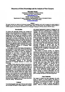
We performed four types of experiments with functional dependencies. As a first type, we executed the regular Conqueror. The second type, denoted ‘disc’ in Figure 1, is Conqueror+ where discovery of dependencies is enabled, but the set of initial provided dependencies is empty. The third type, denoted ‘given’, is Conqueror+ provided with a set of initial dependencies, but without any discovery of functional dependencies. For QuizDB we provided the key dependencies of the QUIZZES and SCORES relations, and for IMDB we provided the key dependencies for ACTORS, GENRES and MOVIES. The fourth type, denoted as ‘given+disc’, is Conqueror+ provided with these dependencies as well as discovery of new functional dependencies.

12

As can be seen in Figure 1a, Conqueror+ with discovery greatly outperforms Conqueror in runtime. This is due to the large reduction in number of queries generated which is clear from the figure. Adding an initial set of (key) functional dependencies results in a small gain in runtime, due to a small reduction in number of queries generated. Similarly, providing a set of dependencies whilst also discovering new ones, results in a small relative gain. We also observe that the exponential behavior of query generation is still present, but only for low support values. Furthermore, for Conqueror+ with discovery, runtime remains almost linear for a large portion of the support values, while for Conqueror, it is increasing rapidly. The experiments on the IMDB shown in Figure 1b show similar results, but in this case, the impact of discovery is smaller. The small amount of attributes in the database reduces the impact of the use of functional dependencies. It is however clear that also in this case, the discovery of functional dependencies reduces the exponentiality of query generation and has an almost linear runtime. Likewise the small impact of providing key dependencies as input to the algorithm, is comparable to QuizDB. We also performed some time analysis to determine the cost of functional dependency discovery. The results for an experiment using QuizDB are shown in Figure 2. It is clear that the time needed for the discovery of functional dependencies (shown as ‘fdisc’ in Figure 2a) is negligible in comparison to the time gained in the selection loop (shown as ‘sel’). Adding discovery also requires extra time in the join loop (shown as ‘join’), but again, the gain in the selection loop outweighs this. Looking at the partitioning of time in Figure 2b, we clearly see that most time is spent in output and input. Since functional dependency discovery in Conqueror+ greatly reduces output and input, we get a large reduction in runtime as was observed in Figure 1.

5

Related Work

Mining frequently occurring patterns in arbitrary relational databases has been the topic of several research efforts. Dehaspe and Toivonen developed the WARMR algorithm [4], that discovers association rules in over a limited type of Datalog queries in an Inductive Logic Programming setting. The input to their algorithm consists of a collection of databases, and then, queries are generated in a level-wise manner, and each candidate query is evaluated against all of these databases. The frequency of a query is the number of databases for which it gives a nonempty answer. Therefore, the interpretation of frequent queries is incomparable to the conjunctive queries considered in this paper. In [6], we studied a strict generalization of WARMR. The notion of diagonal containment provided an excellent tool to compare queries with different sets of projected attributes. Unfortunately, the search space is infinite and there exist no most general and no most specific patterns. However, the subclass of tree-shaped conjunctive queries defined over a single binary relation representing a graph was studied, showing that these tree queries are powerful patterns, useful for mining graph-structured data [7, 10]. In [8], we considered conjunctive queries over several relations, allowing a more efficient algorithm, called Conqueror. Considering projection-selection queries over a single relation, Jen et al. introduced a new notion of query equivalence [13], taking functional dependencies into account,

13

QuizDB support

Q

2000 414

Q (disc)

35 67 105 164 253 412 733

1000 946 700 1362 500 2210 300 3528 200 5656 100 9607

Q (given)

Q (given+disc)

381 907 1279 2097 3344 5405 9216

AR

27 72 113 174 266 457 792

1371 3159 4345 6867 10630 17190 28862

AR (disc)

FD (disc)

46 97 147 234 353 594 1049

AR (given)

AR + FD (dics)

FD (given)

runtime FD (given AR + FD +disc) (given+disc) 17 58 58738

27

73 1293

7

AR + FD AR (given (given) +disc) 1300 41

33

130 3073

7

3080 143

18

161 105323

33

180 4181

7

4188 203

18

221 131603

33

267 6643

7

6650 293

18

311 150602

39

392 10270

7

10277 437

18

39

633 16643

7

16650 807

18

825 244571

39

1088 28139

7

28146 1357

18

1375 265974

Queries

Q (disc)

if given, FDs are: quizzes.quizid->quizzes.name 23 2000 23 quizzes.quizid->quizzes.maker 23 1000 23 quizzes.quizid->quizzes.category 23 700 quizzes.quizid->quizzes.language 23 25 500 29 scores.quizid,scores.name->scores.score 25 scores.quizid,scores.name->scores.maand 300 29 scores.quizid,scores.name->scores.year 33 200 53 109 100 281 753 50 2213 1809 30 5381 3199 20 9543 6605 10 19761

225000

6000 5000

Q (given) 4000

Q (given+disc)

3000 21 21 21 21 2000 21 21 27 1000 23 27 23 0 31 51 0 279 107 2211 751 5379 1807 9540 3196 19758 6602

200

AR

20 20 20 27 27 55 400 321 600 2575 6271 11124 23045

AR (disc)

FD (disc)

15 3 15 3 15 3 15 4 15 4 15 8 800 1400 15 46 1000 1200 minimal support 15 368 15 896 17 1589 17 3292 Association Rules

AR + FD (dics)

AR (given) 18

18 18 18 18 18 19 25 19 25 23 53 1600 1800 61 3192000 383 2573 911 6269 1606 11121 3309 23042

150000

3 3 3 3 3 3 3 3 3 3

FD (given +disc)

AR + FD (given+disc)

runtime

19 16 3 42805 21 3 19 42233 16 21 3 19 42265 16 28 4 20 61632 16 28 4 20 61934 16 56 8 24 63545 16 200 322 400 600 16800 1000 1200 621400 46 63075 1600 2576 368 16 minimal support 384 64742 6272 896 912 65094 16 11124 1589 1606 70177 17 23045 3292 3309 127294 17 Rules

75000

0

0

(a) QuizDB

runtime (disc) runtime (given)

42616 45022 41981 41868 41778 45285 47471 61698 47958 62848 48078 67753 1800 200061468 50483 49525 63508 51096 66522 49514 70289 65904 349586

runtime (given +disc)

jointime

7680000

43655 41476 44848 48154 47456 54675 51647 47858 48766 49379 290889

77 77 77 77 77 77 77 77 77 77 78

30000

AR AR (disc) AR (given) ARQ(given+disc) Q (disc) Q (given) Q (given+disc)

20000

22500 18000 16000

AR AR + FD (dics) AR + FD (given) AR + FD (given+disc) runtime runtime (disc) runtime (given) runtime (given+disc)

Runtime 8100000

22500 milliseconds number of rules

Queries

number of queries number of rules

AR (given +disc) 21

3

30000

?

IMDB AR + FD (given)

FD (given)

14000 15000 12000 10000

7500 8000

8000000

400000

300000

15000 milliseconds

Q

runtime runtime (disc) runtime (given) runtime (given+disc)

7000 milliseconds

support

Q Q (disc) Q (given) Q (given+disc)

8000

number of queries

of which not allowed as constants: quizzes.quizid scores.quizid

runtime (given +disc)

19128 22528 25221 26603 29411 33735 38595

300000

9000

most general projection: quizzen.quizlocatie quizzen.name quizzen.maker quizzen.rubriek quizzen.taal scores.name scores.quizlocatie scores.jaar

455 197775

56645 103394 132648 148833 197775 235013 261444

Runtime

10000 most specific join: quizzes.quizid=scores.quizid

runtime (disc) runtime (given)

18915 22031 24595 25863 30803 32530 36247

7900000

7500

6000

200000

100000

7800000 4000

0

0

2000 0

200

400

600

800

1000

1200

1400

1600

1800

2000

minimal support 0

70

140

210

280

350

420

490

560

630

0

700

0

200

400

600

800

1000

1200

1400

1600

1800

2000

490

560

630

700

minimal support

7700000

0

70

140

210

minimal support

280

350

0

420

(b) IMDB

Association Rules 30000

Association Rules + Functional Dependencies 30000

AR AR (disc) + AR (given) AR (given+disc) +

AR

number of rules

number of rules

AR + FD (dics) Fig. 1: Results for Conqueror, Conqueror with a set of Functional Dependencies given AR + FD (given) AR + FD (given+disc) but22500 no detection (given), Conqueror with only detection of Functional Dependencies 22500 (disc), and Conqueror+ both with given Functional Dependencies and detection. 15000

7500

0

15000

7500

0

70

140

210

280

350

420

minimal support

490

560

630

700

0

0

70

140

210

280

350

420

minimal support

0

70

140

210

28

m

minimal support

490

560

630

700

Output ON In MEM 157,667413 159,8952 354,3541 57,494288 97,92191 39,81962 100,173125 61,97329 95,75927 218,7752

QUIZ DB, discovrey ON, output OFF generateQueries QuizDB

14

Disc

No Discovery 47 29

join proj fdisc sel

15963 17936

Total Algorithms Input Database Communication Output Databases Communication

QuizDB

10 0 3712 9873

total

16010

Algorithm:

QuizDB without DB outpu

27838

11%

Chart 15 join proj fdisc sel

100000 10000 1000 100

Discovery

sel 18,8% 62% fdisc 0,1%

join 0,2%

27%

join proj fdisc sel

No Discovery

36% join 0,1%

sel 35,5%

64% proj 64,4%

10 1

Shop database,

join

Disc

proj

fdisc

sel

total

No Discovery

(a) Time Analysis

proj Algorithms 80,9%

Input Database Communication Output Databases Communication

Algorithms

Input Data

(b) Input/Output Time Analysis In memory QuizDB without DB output

Algorithm Loops

Fig. 2: Time and I/O time analysis of a QuizDB experiment.

16%

17%

39%

which is not the case in previous work. The approach of [13] has been generalised in 61% to a star schema. [14] to databases defined over multiple relations, organised according All approaches other than those discussed just above and dealing with mining frequent queries ([5, 9, 16, 17]) are far more restrictive than ours. Indeed, whereas our approach considers several tables and all possible ways to count supports as distinct Algorithms Input Database Communication values over all possible attribute sets, all these approaches consider a fixed relation to be mined, along with a fixed characterisation of how to count supports. For instance, in [9, 16] tuples are counted, Turmeaux et al. [17] characterize counting by tuple values over a given attributes, whereas Diop et al. [5] characterize counting by a query, called the reference. Notice that all these approaches (except for [17]) are also restricted to conjunctive queries, as is the case in this paper.

6

Concluding Remarks

The contribution of this paper is threefold. First, we combined the results of different prior work resulting in a new algorithm for mining association rules over simple conjunctive queries in arbitrary relational databases, over which functional dependencies are assumed. The algorithm makes use of the functional dependencies of the database to optimise the generation of frequent queries and prune redundant queries. Second, our new algorithm is capable of detecting new functional dependencies that were not given but that hold on the database relations or on any join of these relations. Third, these newly detected dependencies are used to prune even more redundant queries. We implemented our algorithm, and we showed that it greatly outperforms our previous methods and efficiently reduces the amount of queries generated. Several new opportunities for future work exist. First, the additional use of key and foreign key contraints is an issue that we are currently investigating. Other appealing related constraints are conditional functional dependency, introduced by Fan et al. [3]. As these constraints generalise standard functional dependencies using selections, it seems interesting to investigate how they could be used and discovered in our framework.

67%

Join Loop

Projection Loop

15

References 1. R. Agrawal, H. Mannila, R. Srikant, H. Toivonen, and A.I. Verkamo. Fast discovery of association rules. In Advances in Knowledge Discovery and Data Mining, pages 309–328. AAAI-MIT Press, 1996. 2. R. Bocklandt. http://www.persecondewijzer.net. 3. Ph. Bohannon, W. Fan, F. Geerts, X. Jia, and A. Kementsietsidis. Conditional functional dependencies for data cleaning. In ICDE, pages 746–755, 2007. 4. L. Dehaspe and L. De Raedt. Mining association rules in multiple relations. In 7th International Workshop on Inductive Logic Programming, volume 1297 of LNCS, pages 125–132. Springer Verlag, 1997. 5. C.T. Diop, A. Giacometti, D. Laurent, and N. Spyratos. Composition of mining contexts for efficient extraction of association rules. In EDBT’02, volume 2287 of LNCS, pages 106–123. Springer Verlag, 2002. 6. B. Goethals and J. Van den Bussche. Relational association rules: getting warmer. In ESF Exploratory Workshop on Pattern Detection and Discovery in Data Mining, volume 2447 of LNCS, pages 125–139. Springer, 2002. 7. B. Goethals, E. Hoekx, and J. Van den Bussche. Mining tree queries in a graph. In ACM KDD, pages 61–69, 2005. 8. B. Goethals, W. Le Page, and H. Mannila. Mining association rules of simple conjunctive queries. In SIAM-SDM, pages 96–107, 2008. 9. J. Han, Y. Fu, W. Wang, K. Koperski, and O. Zaiane. Dmql : A data mining query language for relational databases. In SIGMOD-DMKD’96, pages 27–34, 1996. 10. E. Hoekx and J. Van den Bussche. Mining for tree-query associations in a graph. In IEEE ICDM), pages 254–264, 2006. 11. IMDB. http://imdb.com. 2008. 12. A. Inokuchi, T. Washio, and H. Motoda. An Apriori-based algorithm for mining frequent substructures from graph data. In PKDD, volume 1910 of LNCS, pages 13–23. Springer, 2000. 13. T.Y. Jen, D. Laurent, and N. Spyratos. Mining all frequent selection-projection queries from a relational table. In EDBT’08, pages 368–379. ACM Press, 2008. 14. T.Y. Jen, D. Laurent, and N. Spyratos. Mining frequent conjunctive queries in star schemas. In International Database Engineering and Applications Symposium (IDEAS), pages 97– 108. ACM Press, 2009. 15. M. Kuramochi and G. Karypis. Frequent subgraph discovery. In IEEE ICDM, pages 313– 320, 2001. 16. R. Meo, G. Psaila, and S. Ceri. An extension to sql for mining association rules. Data Mining and Knowledge Discovery, 9:275–300, 1997. 17. T. Turmeaux, A. Salleb, C. Vrain, and D. Cassard. Learning caracteristic rules relying on quantified paths. In PKDD, volume 2838 of LNCS, pages 471–482. Springer Verlag, 2003. 18. E.W. Weisstein. Restricted growth string. In From MathWorld – A Wolfram Web Resource (http://mathworld.wolfram.com/RestrictedGrowthString.html), 2009. 19. X. Yan and J. Han. gspan: Graph-based substructure pattern mining. In IEEE ICDM, page 721, 2002. 20. M.J. Zaki. Efficiently mining frequent trees in a forest. In ACM KDD, pages 71–80, 2002.