then sent to a central domain server where it is decomposed in order to retrieve the necessary aggregate data from the distributed database. This is carried out ...
Discovery of Multi-level Rules and Exceptions from a Distributed Database Rónán Páircéir
Sally McClean
Bryan Scotney
School of Information and Software Engineering, Faculty of Informatics, University of Ulster, Cromore Road, Coleraine, BT52 1SA, Northern Ireland.
++44 (2870) 324366
{r.pairceir, si.mcclean, bw.scotney}@ulst.ac.uk heterogeneous DBMS [1]. In Europe a convergence between Database Technology and Statistics has been particularly encouraged by the EU Framework IV initiative, with DOSIS projects IDARESA [2] and ADDSIA [3], which retrieve aggregate data from distributed statistical databases via the internet. These projects store data with a large amount of associated domain knowledge in the form of statistical metadata, which lends itself nicely to the task of knowledge discovery incorporating this domain knowledge.
ABSTRACT Large amounts of data pose special difficulties for Knowledge Discovery in Databases. Efficient means are required to ease this problem; this can be achieved using sufficient statistics rather than individual level data. Sufficient statistics are especially appropriate for Knowledge Discovery from distributed databases, where it may be either too expensive or prohibited by confidentiality constraints to communicate individual level data across the network. The data of interest are of a type similar to those found in OLAP data cubes and Data Warehouses. They consist of both numerical and categorical attributes (dimensions) and are contained within a hierarchical structure. There are few algorithms to date that explicitly exploit this hierarchical structure when carrying out knowledge discovery on these data. Using sufficient statistics in the form of aggregate data and accompanying statistical metadata retrieved from a distributed database, we use multi-level models to identify and present relationships between a single numerical attribute and a combination of other attributes at various levels of the hierarchy. On the basis of these relationships, rules in conjunctive normal form are induced. We present to the user the significant attribute relationships and interactions via a graphical interface rather than the traditional statistical table. Exceptions to these rules are discovered, and the user may browse these exceptions at different levels of the hierarchy.
In order to alleviate some of the problems associated with mining large amounts of individual level (micro) data, one option is to use a set of sufficient statistics in place of the data itself [4]. This is particularly important in the distributed database situation encountered in both IDARESA and ADDSIA, where issues associated with slow data transfer and confidentiality constraints may preclude the transfer of the individual level data [5]. In this paper we show how the same results can be obtained by communicating aggregate data from each site to a central site in place of the individual level data. This has two associated problems; firstly deciding on the sufficient statistics in the form of the aggregate data which need to be communicated from each site in order to compute a required model; secondly ensuring that these distributed sufficient statistics can be combined centrally in a meaningful way. The types of data we deal with here are similar to the multidimensional data stored in a Data Warehouse (DW) [6,7]. These data consist of two attribute value types: measures or numerical data, and dimensions or categorical data. Some of the dimensions may also have associated hierarchies to specify grouping levels. This paper deals with such data in statistical databases, but should be easily adapted to either a typical or a distributed DW implementation [8].
Keywords Multi-level Statistical Models, Aggregates, Distributed Databases, Sufficient Statistics, Exception Discovery, Rule Discovery.
1. INTRODUCTION
In our database implementation, the individual level or micro data is stored in Fact and Dimension tables on the different sites using the STAR relational schema [6]. The aggregate data is stored in the form of MAMED Objects [3], consisting of two parts: a macro relation (containing the aggregate data) and its corresponding statistical metadata relations (containing statistical metadata for tasks such as dimension value re-classification, measure value conversion and statistical model computation). Using this aggregate data, it is possible, with models taken from the field of statistics, to study the relation between a single measure attribute and a combination of one or more explanatory attributes from various levels of a hierarchy. We demonstrate this approach using statistical multi-level models [9, 10, 11] which enable us to relax many of the constraints normally associated
Frequently data are distributed on different computing systems in various sites. Distributed Database Management Systems provide a superstructure which integrates either homogeneous or
Permission to make digital or hard copies of part or all of this work or personal or classroom use is granted without fee provided that copies are not made or distributed for profit or commercial advantage and that copies bear this notice and the full citation on the first page. To copy otherwise, to republish, to post on servers, or to redistribute to lists, requires prior specific permission and/or a fee. KDD 2000, Boston, MA USA © ACM 2000 1-58113-233-6/00/08 ...$5.00
523
These details form the user's query on a client site. This query is then sent to a central domain server where it is decomposed in order to retrieve the necessary aggregate data from the distributed database. This is carried out by a Query Agent which sends out MAMED Object requests to the relevant distributed sites. The required data is then used to construct the multi-level model.
with statistical models. Thus in this paper, we illustrate how a user may obtain rules and exceptions from data which is distributed over a number of sites. This follows on from difficulties workers in statistical agencies were having in building models and obtaining knowledge from data which was geographically dispersed over databases in a number of countries. They were also faced with confidentiality considerations in communicating the individual level data from other statistical agencies and other approaches were required to solve this problem.
A multilevel problem is one that concerns the relationships between attributes that are measured at a number of different hierarchical levels. For the example data above, the user is attempting to discover rules and exceptions for the attribute "Cost of insurance claims" based on a number of individual level attributes, a number of attributes at a regional level and a further set of attributes at a country level indicated in Table 1.
The following section, Section 2, contains an extended example and an explanation of the multi-level problem structure. Section 3 shows how the data are retrieved and integrated in preparation for the multi-level model building phase. Multi-level modeling and computation are discussed in Section 4, along with the method of presenting the resulting discovered knowledge in Section 5. Section 6 concludes with related work, summary and possibilities for further work.
Table 1.
Attribute COST OF CLAIM CLAIM TYPE GENDER AGE CAR-CLASS PREVIOUS CLAIMS DRIVER TEST SCORE YEARLY MILEAGE REGION NAME REGION TYPE MANDATORY CAR TESTING REGIONALAL ROAD ASSESMENT SCORE COUNTRY NAME DRIVER LOWER AGE LIMIT MEAN COUNTRY CLAIM
2. AN EXTENDED EXAMPLE AND THE MULTI-LEVEL PROBLEM STRUCTURE To illustrate our approach we present an insurance example where the data are stored in databases on four different distributed sites in Ireland, England, France and Spain. These data are distributed horizontally with some attribute domain value mismatches over the different sites which need to be redressed before the modeling phase. The database schema for the micro data is shown in Figure 1 along with the concept hierarchy showing that Individual driver data are nested within Regions within Countries. The attributes of interest to the user are shown in Table 1. Mean Country Claim in Table 1 is a derived attribute, calculated when the data are aggregated.
BaseTable BaseID ClaimType Gender Car-Class PreviousClaims
Figure 1.
FactTable DateID RegionID BaseID Cost Age Score Mileage
RegionTable RegionID R-Name R-roadScore R-Type
DateTable DateID Year Month Day
Attributes of interest in the modeling phase Values {Continuous} {Accident, Theft} {Male, Female} {Continuous} {A, B, C} {Yes, No} {Continuous} {Continuous}
Level Individual Individual Individual Individual Individual Individual Individual Individual
{City, County} {Yes, No}
Region Region
{Continuous}
Region
{16, 18}
Country
{Continuous}
Country
Once groupings exist (e.g. drivers from the same country or region) the individual tuples may not be independently and identically distributed (IID). Heterogeneity is very often present in relationships between hierarchical data held in databases, and frequently the statistical models with full IID assumptions do not explain this heterogeneity sufficiently. If this independence assumption is violated, the estimates of the standard errors of conventional statistical tests are much too small, resulting in many deceptive statistically significant results. This lack of independence between observations within groups is expressed as the intra-class correlation. It is a population estimate of the variance explained by the grouping structure.
Country
Region
Individual
Concept Hierarchy
Multilevel models [9] attempt to realistically model these situations where there is clustering of individuals within groups and attributes are measured at different grouping levels of the hierarchy. They essentially work by combining models which are built at each level of the hierarchy. In these models the assumption of independence of individuals is dropped, and relationships in the data are no longer assumed to be fixed over groups but are allowed to differ.
Star Schema of micro data and Concept Hierarchy
The process begins with the user browsing through textual statistical metadata held in XML [12] to select a set of measures (possibly specifying some derived measures) and dimensions of interest, along with an appropriate model. The user may also specify restrictions on the attribute values of interest (e.g. selecting "GENDER=Female" or "Cost of Claim >£5000").
524
statistical metadata [3] required for example for harmonisation of the data at the central domain server. This view of micro and macro data is similar to the base data and materialised views held in a Data Warehouse [6]. In addition, in the ADDSIA system [12], textual (passive) statistical metadata for use in documentation are held in XML files. These textual statistical metadata can be browsed by the user as an aid to choosing a relevant set of attributes to model. They may also contain domain knowledge to assist the user in the form of previously discovered relationships in the data. Storing the micro data in the relational STAR schema format [6] as shown in Figure 1 reduces the time required for query execution in producing the required macro relations [7]. The aggregate data in our system is stored in a single relational table format.
In this paper we use multilevel models with a number of goals in mind: •
firstly to determine the direct relationships between a single measure attribute (cost of insurance claim) and a number of individual and group level explanatory attributes (e.g. age, region type).
•
secondly to determine if the explanatory attributes at the group level (regional and country attributes) serve as moderators of individual level relationships. If such moderators exist, they show up as statistical interactions between explanatory attributes from different levels. This would occur, for example, if varying the regional road assessment score affected the relationship between yearly mileage and claim cost at the individual level. Such moderator or interaction relationships also allow us to explain some of the variation in the cost of insurance claims between groups (regions and countries). This is not possible using other statistical techniques. As an example, if there is a stark difference in the individual level cost claims between certain regions, it may be possible to explain this difference in the multilevel model using some of the region level attributes (for example whether the region is a city or a county).
•
thirdly to improve prediction of cost claims within individual units [11], especially for minority groupings by pooling similar individuals from different groups.
•
fourthly to partition the variance components among levels into between-group (how much of the variation in claim costs can be put down to differences in drivers from different regions) and within-group components (how much of this variation is due to differences between drivers within the same region).
•
Graefe et al. [4] state that "most algorithms are driven by a set of sufficient statistics that are significantly smaller that the data". Their approach takes advantage of the query processing system of SQL databases to produce a set of sufficient statistics for classification, thereby avoiding the need to move the individual level data to the client. This results in a significant increase in performance. In the distributed database situation, where it may be too expensive or prohibited by confidentiality constraints to communicate the individual level data across the network, obtaining such a set of sufficient statistics is even more relevant. However in the distributed database scenario, we must not only find a set of sufficient statistics for the statistical models we wish to construct, but we must also ensure that they can be combined at the central site in a meaningful way. For the statistical models we use, our sufficient statistics consist of aggregates in the form of counts, sums and sums of squares of measures and products of measures. These aggregates also serve as sufficient statistics to a number of other statistical procedures including Analysis of Variance Models, Regression Models and other linear statistical models. With this in mind, the data model for MAMED Objects was developed to store these sufficient statistics which are calculated from the micro data. A single MAMED Object consists of a macro relation with a number of accompanying statistical metadata relations [3]. The statistical metadata relations associated with a single macro relation in a MAMED Object [3] consist of a set of relational tables required for statistical model building and data harmonisation and integration at the central domain server. They include statistical population estimation information, reclassification information for measures and dimensions, and statistical modeling information.
lastly to isolate groups at different levels of the hierarchy that represent exceptions.
On the basis of the relationships discovered using such multilevel models, we induce rules in conjunctive normal form. Exceptions to these rules are also discovered, and the user may browse these exceptions at the different levels of the hierarchy. For example we may uncover a rule that states that cost claims for males in Ireland can be expected to lie within a given range. Following on from this, we may find an exception grouping of males in region 12 in Ireland where the claim costs lie outside this range in a statistically significant way. This may then lead the user to an investigation of this region and eventually to conclude that the cost of insurance for males in this region needs to be higher to cover the extra claim costs (due perhaps to higher than average car theft in the region). Without the statistical metadata in our system which indicates the hierarchical level of each attribute, the data could only be analysed at the individual level, with all higher level attributes stepped-down to this level. This metadata is even more important if the multilevel models are to be computed in an automated fashion.
Within a MAMED Object a macro relation R describes a set of macro objects (statistical tables) where C1,..Cn represent n dimensions and S1,…Sm are m sets of summary attributes. Each Si in the macro relation consists of aggregates in the form of count (N), sum (SM) and sums of squares (SS) for a measure or derived measure from the micro data. The aggregates in each set of summary attributes are functionally defined by a cross product of the dimension attribute domain values. As an example, Table 2 shows a macro relation with two dimension
3. AGGREGATE DATA RETRIEVAL AND INTEGRATION The data at any one site can consist of individual level “micro” data and/or aggregate “macro” data, along with accompanying
525
Table 2. Macro relation for Gender and Claim Type for Ireland 1998 Gender
Claim Type
Age_N
Age_SM
Age_SS
Derived_N
Derived_SM
Derived_ SS
Male
Accident
4240
148428
5194534
4240
1763.84
733.75
Male
Theft
1341
45594
1550196
1341
894.35
595.40
Female
Accident
2210
70720
2263040
2210
464.10
97.46
Female
Theft
956
26768
749504
956
1195.34
1493.75
attributes (gender and claim type) and two measures (age and a derived measure claimcost divided by yearly mileage). The cross product of the dimension attribute values results in four records, each with its corresponding set of summary attribute sets for each measure.
attributes with the same domain set (e.g. the French database might classify Accidents in Claim Type as “Accident Type A” and “Accident Type B” separately. These need to be reclassified and aggregated using a MAMED operator to the single value “Accident” which is the appropriate classification used by the other Countries involved in the query). Another MAMED operator is used to convert all of the measures' values to common units (e.g. all claim costs need to be converted to the common currency of EUROs). The final harmonised MAMED Objects from each site now contain macro relations which are domain compatible and can therefore be integrated into a single aggregate macro relation. The statistical metadata relations are also integrated accordingly, and the user can view these if required to see how the final macro relation was obtained. The final task is to apply the DATA CUBE operator [14] to all of the N, SM and SS summary attributes in the macro relation. The data is now in a suitable format for the statistical modeling phase.
The concept which enables us to combine the summary attributes from the distributed macro relations to form a centralised set of sufficient statistics for the multi-level model is the additive property of these summary attributes [13]. This property allows us to combine aggregate data from the distributed sites seamlessly and is defined in (1) as follows: σ ( α UNION β) = σ (α) + σ (β)
(1)
where α and β are macro relations which are domain compatible and σ() is an application of an additive summary function (e.g. SUM) over a measure in α and β. Two macro relations are deemed to be domain compatible if they contain the same dimension attributes, each with identical domain sets, and the same summary measures, each defined on the same units. Thus an England 1998 macro relation which is domain compatible with the Ireland 1998 macro relation in Table 2, would also contain four entries and identical summary measures with the same units. The function MEAN is not an additive summary function and for this reason our summary measures do not include Mean values. However, with the Counts and Sums, we can for example obtain the mean age of all Gender=females over the two countries by dividing the sum of the appropriate Age_SM values for the two countries by the sum of their corresponding Age_N (Count) values.
In this way it is possible to combine aggregates over these summary attributes in distributed macro relations at a central site for our knowledge discovery purposes, once the data have been suitably harmonised using the statistical metadata relations. This also enables us to leverage the query processing system of SQL databases (including the Data Cube operator) to compute our sufficient statistics in the form of the aggregates held in the final macro relation. By communicating only these aggregate data, we overcome the problems associated the confidentiality constraints in communicating individual level data across the network.
3.1 Implementation Issues
To retrieve aggregate data in a domain compatible format from the distributed data sites, a complete set of operators has been developed to work with MAMED Objects [3]. These MAMED operators are implemented using SQL and operate simultaneously on a macro relation and on its accompanying statistical metadata relations. In this way the statistical metadata relations only contain information relevant to the attributes which are in the corresponding macro relation. Thus if a measure or a dimension is removed from a macro relation, information pertaining to those attributes is also removed from the statistical metadata relations.
In our prototype the micro data and MAMED Objects are stored in INGRES DBMS on each site. Access to remote distributed servers is achieved via the Internet in a Java environment. A well-acknowledged three-tier architecture has been adopted for the design. The logical structure consists of a front-end user (the client), a back-end user (the server), and middleware which maintains communication between the client and the server. The distributed computing middleware capability remote method invocation (RMI) is used here. A query is transformed into a series of nested MAMED Operators and passed to the Query Agent for assembly into SQL and execution.
Once the initial required MAMED Objects have been created at each site from the micro data (or from pre-existing MAMED Objects), they are communicated to the Domain Server. Here MAMED operators are applied to the macro relations using information in the statistical metadata relations so that the macro relations are domain compatible and ready to be integrated together. In many cases a dimension’s domain values need to be reclassified so that all the macro relations contain dimension
4. MODELING PHASE 4.1 Multilevel Models The multilevel models used may be exemplified using a two level hierarchy consisting of individual drivers and regions from the
526
insurance problem in Section 2. This model1 can be extended to more levels and more attributes at each level [15]. At the individual driver level we use Gender (X1) and DriverTestScore (X2) to predict Cost of Insurance Claim(Yij) for driveri in regionj. At the regional level we include attributes Region Type (Z1) and Road Assessment Score (Z2). The full multi-level may be explained by dividing up the model into equations (2), (3) and (4). Initially a separate model can be built for each regionj, with separate slopes (β0j) and intercepts (β1j, β2j) as shown in (2).
4.2 Computing a Normal Iterative Generalised Least Squares Solution The matrix notation for the two level multi-level model is Equation (5) is shown below. X is a matrix of the attribute and attribute interaction values, Y is a matrix of the corresponding cost claims, β is a matrix containing the model coefficients and V is a Block Diagonal covariance Matrix [15] containing the variance and covariance components of the model.
Yij = β0j + β1jX1ij + β2jX2ij + εij (2)
1 1 X = 1 .. 1
where β0. is the usual regression equation intercept, β1. and β2. the usual regression slopes and εij the usual residual error term. Yij represents the claim cost of an individual driveri within regionj. The model in (2) which is termed a level 1 model, differs from a regression model in that both the intercepts and slopes are allowed to vary across regions. Thus across all regions, each of these slope and intercept coefficients have a mean and variance, and in the multilevel model the variation in these coefficients is modeled by introducing explanatory attributes at the Region Level (Z1 and Z2). To model the variation in the intercept coefficients across regions, level 2 models are introduced as shown in (3) and (4).
1 ij
x 1 11 x 1 21 .. x 1 nm
X
2 ij
.. x 2 nm
Matrix of model β = coefficien ts
..
..
X 2 Z 2 ij x 2 z 2 11 x 2 z 2 21 .. x 2 z 2 nm
Yij y11 Y = .. .. ynm
Block Diagonal V = covariance matrix
Maximum Likelihood [9] is used to obtain estimates of the fixed and random coefficients of the model. Computing the maximum likelihood estimates requires an iterative procedure, iterating from estimating the fixed components (β), to using these estimates to estimate the random components (V), which in turn are used to estimate the fixed components in the next iteration. In this paper we use an iterative generalised least squares method (IGLS) [15] to compute these fixed and random components. This method begins by generating reasonable starting values for the β estimates, based on simple single-level ordinary least squares (OLS) regressions (Equation (6) with the V-1 matrix terms removed and higher level random effects (µ0j and µhj) assumed equal to zero). The resulting β estimates from Equation (6) are used to obtain a matrix G of raw residuals (differences between the observed claim costs,Yij, and predicted values computed using the β estimates for each individual). In the second stage of an iteration, this matrix G is used in conjunction with structural information on the V matrix, to obtain estimates of the random components in the V matrix also using GLS [15] of a similar form to Equation (6). The iterations continue in this way using refined estimates of the random components (V) matrix in Equation (6) to obtain improved fixed components (β) estimates until the process converges.
β0j = γoo + γo1Z1j+γo2Z2j + µ0j (3) and for each slope coefficient (β1j, β2j) for h∈{1,2} βhj = γh0 + γh1Z1j+γh2Z2j + µhj
X
(4)
where γoo,γho are intercept coefficients, γo. and γh. the slope coefficients and, µ0j and µhj the residual errors at the region level. All level 2 residual errors are assumed to have a mean of zero and to be independent from the residual errors at level 1 in (2). Hence equation (3) states that the variation in the level 1 intercept coefficient (β0j) can possibly be explained by the level 2 attributes Z1 and Z2, with any residual error variance being captured in µ0j. Equation (4) states that the variation in the level 1 slope coefficients (βhj) can possibly be explained by attributes Z1 and Z2, with any residual error variance being captured in µhj. By substituting Equations (3) and (4) into Equation (2) for β0j, β1j and β0j, we obtain a single complex equation giving us a multi-level model at two levels shown in Equation (5). This can be generalised to a case with more levels and more explanatory attributes at each level, as well as interaction terms at level 1. Equation (5) breaks the model into a fixed components part and a random components part.
β = (XTV-1X)-1 XTV-1Y
(6)
Y ij = [γoo + γ10X 1ij + γ20X 2ij + γo1Z 1j
4.3 Replacing Individual Level Data with Aggregates in GLS
+ γ o2Z2j + γ11X 1ijZ 1j+γ 12X 1ijZ2j + γ 21X 2ijZ1j+γ 22X 2ijZ2j] + [µ2jX 2ij + µ1jX 1ij + µ0j + ε ij]
1
In [16] we show how the aggregate data in the macro relations can be communicated as sufficient statistics in place of the individual level data to compute ANOVA models. Computing an ANOVA model requires only one MAMED Object to be retrieved from each distributed site. Here we show how this can be achieved for multilevel models, but we require more than one retrieval of MAMED Objects. While it is not the focus of this paper to
(5)
There are many variants on these models depending on the data characteristics.
527
describe the computational methods used in great depth, sufficient detail is included in order to provide an understanding of the process.
Applying This Approach to IGLS for 4.4 Distributed Data
Both stages of an iteration in computing a multi-level model involve GLS as indicated in section 4.2 for the case where the individual level data is available centrally. To see how we can
Having shown in section 4.3 that the aggregate data from the macro relations can be used to solve a multilevel problem with IGLS, this must be applied to the distributed data. Each iteration of the IGLS requires a number of communications of data and requests for data between the distributed sites and the domain server. This series of steps is illustrated in Figure 2.
∑V X = β ∑V β ∑V X ∑V X Y = β ∑V X β ∑V X i
i
i
i i
i +
0
0
i
∑Vi X TV −1 X = ∑Vi X i
1
i +
i
1
i
∑Vi X i 2 ∑Vi X i
∑ Vi Yi X T V −1Y = ∑ Vi X i Yi
(7)
i
2 i
(8) Step 1. MAMED Object requests sent from Query Agent to distributed sites. MAMED Objects computed and returned to the central domain server where they are harmonised, integrated and Cubed.
(9)
Step 2.
(10)
The aggregate matrices containing the required aggregates are assembled from the final Macro relation and used to calculate the initial fixed component β estimates using Ordinary Least Squares.
accomplish this by communicating only aggregate data to and from the central domain server, we take the simplest GLS model (equation (6)) consisting of only one X attribute. The generalised least squares normal equations (derived by calculus [17]) used to solve this simple GLS model are shown in equations (7) and (8). The Vi are matrix elements from the V-1 matrix in equation (6). Using the least squares normal GLS equations (7 and 8), it is possible to obtain a more compact representation for the matrix equation in (6) in terms of aggregates. This is shown in equations (9) and (10). We call the two matrices in (9) and (10) aggregate matrices. The matrix elements in (9) and (10) consist of sums and sums of squares of attributes (and products of those attributes).
Step 3. The resulting fixed component β estimates are communicated to each distributed site and used to compute new MAMED Objects consisting of aggregates of raw residuals for the G matrix. Step 4. Each site's raw residuals G matrix aggregate components are returned to the domain site, harmonised, and used to assemble the necessary aggregate matrices required to calculate the random component V matrix using Generalised Least Squares.
These aggregate matrices form the set of sufficient statistics for the GLS estimation procedure. Using our MAMED Operators as explained in Section 3, it is possible to assemble these aggregate matrix elements centrally from the original distributed individual level data, by communicating only the relevant aggregate data. When the retrieved aggregates are harmonised and integrated, they can be fitted into the matrices in equation (9) and (10) and then used to solve equation (6). This simple example can be generalised to the more complicated equations we face when solving a GLS for a mulit-level model and the result is the same: that we can solve a GLS equation using only aggregate data retrieved from the distributed sites.
Step 5. The relevant components of the V-1 inverse matrix of random components are communicated from the domain server to each distributed site and a new MAMED Object incorporating this V-1 data is computed for the next iteration estimation of theβ fixed component matrix at the domain site.2 This process then returns to Step 2 and continues in an iterative fashion from refined β estimation to refined V estimation until convergence. After iteration 1, OLS in Step 2 replaced by GLS.
Such aggregate matrices can be used to compute both the fixed component β coefficient estimates and the random component V components for any IGLS iteration, since both stages employ the same GLS methods. However since the Vi estimates in the V-1 matrix change after each iteration, the matrix aggregates represented in (9) and (10) need to be recalculated from the micro data each time. The same applies to the computation of an aggregate G matrix for the random component estimation part of an iteration. This implies that in the distributed case, a number of communications between the central domain server and the distributed sites are required for each iteration of the IGLS. This is the focus of the following section.
Figure 2.
Steps involved in IGLS from distributed database
Currently in our system, the user specifies the particular multilevel model of interest. An automated approach allows the
2
528
Aggregates in matrices (9) and (10) or their more general versions require sums of products of individual elements of the X matrix and the V-1 matrix which must be computed at the distributed sites. It is for this reason that the V-1 matrix must be communicated to the distributed sites.
Figure 3. Attribute significance and Breakdown of Variance between levels effect or the ecological fallacy. Robinson also showed that drawing inferences at a higher level from an analysis at a lower level can be just as misleading. This is known as the atomistic fallacy. Therefore these techniques would be unsuitable in this case.
user to simply select attributes which may be of interest and the system automatically builds the best model from this given set of attributes. Work on the automated approach is at an early stage and is not described further here.
4.5 Alternatives to Using Multi-level Models
5. RESULTS PRESENTATION
Historically multilevel problems were handled by analysing all attributes at one single level of interest. This was accomplished by either stepping-up3 or stepping-down to an appropriate hierarchy level and computing the model at that level using multiple regression techniques. Stepping-up a level implies carrying out the analysis at a level higher than the individual level. For example if we step-up to the region level, the analysis is carried out at this level and the means of the individual level attributes in each region are used in place of the individual level values. If the analysis is carried out at the individual level, stepping-down a level implies moving region and country level attribute values from being descriptors of these groups, to being descriptors of the individual tuples.
Once the model parameters have been calculated and validated for appropriateness, the results are presented to the user. Our approach summarises the main details of this output in a format more suited to a user not overly familiar with statistical modeling and analysis. This begins with a graph as shown in Figure 3, containing only those explanatory attributes or effects from the various hierarchical levels which exhibit a statistically significant relationship with Cost of Insurance claim. The higher the bar, the greater the statistical significance of the relationship. Presenting the standardised effects initially in Figure 3 allows the user to compare the statistical significance of the attribute relationships against each other on a common scale. By clicking on the bottom left-hand button in Figure 3, the user may view the significant effects on an un-standardised scale. These values are more important in terms of the real effect of the significant attributes on the insurance cost claims. This information is also conveyed to the user in more detail in the form of rules. There is a significant cross level interaction effect indicated between the region level attribute region type and yearly mileage from the individual level. This means that the relationship between yearly mileage and insurance claim cost is also dependant on the associated value of region type.
However, while these strategies would be very efficient computationally for our purposes as they do not require an iterative solution, they create two different sets of problems. Kreft [11] states that the within-group information can account for as much as 80-90% of the total variation in such data. Therefore by stepping-up to a higher hierarchy level, this information would be lost before the analysis has even begun. Stepping-down can lead to many apparent statistically significant relationships that are in reality questionable [10]. There can also be problems associated with analysing all of the data solely at one level and drawing conclusions about the relationships at another level. Robinson [18] shows that relationships between means of individual level attributes for example, can not be used as estimates for the corresponding individual-level relationships. This is known as the Robinson
3
The user can interact fully with this graphical output to interrogate the results at more detailed levels. This allows the user to understand an effect’s relationship with the cost of insurance claim in greater depth. By clicking on one of the level options in the legend, the user can view a tabular representation of the statistical significance of all the explanatory attributes included in the model at that level, or for all interactions included in the model. For significant dimension and measure attributes not involved in interactions, it is possible to isolate their effect on the cost of insurance claim while holding all of the other attributes values constant. For dimensions, this is accomplished by drilling down to the attribute domain value level, presented both
In multilevel modeling the traditional terms used for "steppingup" and "stepping-down" are "aggregation" and "disaggregation". We do not use the traditional terms here in order to avoid confusion as we use the term aggregation elsewhere in another context.
529
Car-Class {Type A} → cost of insurance claim between {1700.4 - 2148.4} Car-Class {Type B} → cost of insurance claim between {1161.4 - 1582.4} Car-Class {Type C} → cost of insurance claim between {1039.4 - 1487.4}
Figure 4. Graph of cost claims broken down by Car class and associated rules graphically and in rule format (in conjunctive normal form). This is accomplished by clicking on the bar of an attribute of interest in Figure 3. As an example, by clicking on the Car-Class bar, the graph and corresponding rules in Figure 4 appear. This shows a breakdown of average insurance claim costs for each car-class. The graph illustrates this for each car-class in terms of deviance in claim cost from the overall average claim cost. The rules present this information with associated statistical confidence intervals. From the rules, it can also be seen that there is a statistical difference between cost of claims for car-class C and the other classes, while there is no statistically significant difference between the cost of insurance claims between drivers in carclasses A and B. This illustrates at a lower more detailed level, the relationship between car class and cost of insurance claims. The user could then, after further investigation, decide to charge drivers of car class A a higher premium to cover this extra cost.
% of the overall variation in cost of insurance claims which is between regions within countries
Type 3.
% of the overall variation in cost of insurance claims which is between countries
This information is also presented to the user in Figure 3. In the insurance data, 33% of the variation was of type 1, 24% was of type 2 and a large 43% of the variation was of type 3 between countries. These figures aid the user in determining where most of the variation in the cost of insurance claims arises.
5.2 Finding Exceptions to the Induced Rules The final pieces of knowledge which are automatically presented to the user are exceptions to discovered rules. A rule is something which holds for a grouping of drivers or observations. An exception to a rule represents a single driver, or a minority grouping of the drivers covered by a rule, who behave in a manner which is significantly different from the majority of the grouping in some sense. More specifically, the term “exception” here is defined as an individual or aggregate measure value which differs in a statistically significant manner from its expected value calculated from the multilevel model. The exceptions (as is the case for the rules) are presented in conjunctive normal form, along with the actual cost of insurance claim (an average if it involves a group of drivers rather than an individual driver) and the expected cost (from the model) in terms of a confidence interval. A simple example is an exception grouping defined as:
Effects are interpreted differently for explanatory attributes which are measures. These are presented as rules where a one unit increment in the explanatory measure, holding all other attribute values constant, brings about a certain increase or decrease in the cost of insurance claim. These rules are also presented with an associated confidence interval. For attributes involved in an interaction effect, if all or some of the attributes are measures, the rules resulting are similar to those for measures (but having more conjunctions). If the interacting attributes in an effect are all dimensions, the rules are similar to those for a dimension effect (again having more conjunctions) and a graph similar to Figure 4 is also presented to the user, broken down for each combination of the cross product. As a final step, the user can view all resulting rules together. The combined set of rules summarise the discovered knowledge. In this way, the user can browse through the results, moving from a high-level graphical representation of the attribute level information, to lower more detailed levels.
[Country {Ireland} ∧ Car-class{A} ∧ Region {City} ∧ Claim Type {Theft} ∧ Gender {Male}, predicted cost claim {1820.54-2023.54 ECU}, actual average cost (11) claim 2100 ECU]
Taking information from the final V matrix coefficients produced by the multilevel model, a graph of the statistically significant variation components within each level is presented to the user. For the insurance problem this can be divided into the following variation components: Type 1.
Type 2.
This grouping can be deemed to be an exception as the actual claim cost lies outside the range as predicted by the multilevel model. This exception can be investigated by the user. One factor which is also important to a user interested in finding exceptions, is to know in what way they are exceptions. The user may possibly be given some guidance in this quest through an examination of the rules which are related to the exception. We
% of the overall variation in cost of insurance claims which is between drivers within regions
530
define a rule and an exception to be related if the rule antecedent is nested within the exception antecedent. If we assume that as well as the rule set in Figure 4, we also have a rule as shown in (12),
7. SUMMARY AND FURTHER WORK In summary, we have described a means of discovering rules and exceptions from hierarchically structured data returned from a number of databases distributed over the internet. We have shown how it is possible to use a set of sufficient statistics in place of the individual level data to build such multilevel models over a distributed database. We have also illustrated ways in which the knowledge represented in the model can be presented to the user at different levels of detail. Further work will involve the intelligent automatic building of a good multilevel model where only the attributes of interest are specified by the user. Since this will involve many more iterations than the current implementation, efficient means will be required for this process. One possibility is the use of random sampling of the distributed data to build initial models. Other possible algorithms and data mining tasks which could take advantage of the aggregates will also be investigated.
Region Type {City} → Cost of Insurance claim {924.20 - 2124.60}
(12)
it can be stated in this simple illustration that car-class is in some sense a causal factor in exception (11), as the actual cost of insurance claim 2100 ECU exceeds the range of car-class A's rule, but not that of the rule in (12). This may conveys more knowledge to the user about the exception. Further work is required on this last concept to automate the process in some suitable way. Before making any decisions, this exception should be investigated in detail by the user. If it is found to be a data error of some sort, it should be removed from the data and the model rebuilt. Otherwise it should remain in any model building. Due to the confidentiality constraints associated with our distributed data, it may not be permitted to discover such exceptions at the individual level of the data and therefore such exceptions may be discovered at aggregate levels only. As a final note, if the model is to be used for prediction purposes, it is beneficial to split the data into a test set and a training set similar to decision tree building in order to obtain a more robust model [17].
8. ACKNOWLEDGEMENT This work has been partially funded by ADDSIA (Esprit project no. 22950) which is part of EUROSTAT's DOSIS initiative.
9. REFERENCES [1] [2]
6. RELATED WORK Multilevel models have also been used for consumer purchasing behaviour. [19] uses multilevel models to look at the purchase and use of personal care products in terms of product use profiles. Of primary interest was the variation in behaviour between individuals. In the area of supervised learning, a lot of research has been carried out on the discovery of rules in conjunctive normal form and some work is proceeding on the discovery of exceptions and deviations for this type of data [20, 21]. A lot less work in the knowledge discovery area has been carried out in relation to a measure attribute described in terms of either dimension attributes alone or a combination of dimensions and measures at levels in a hierarchy. Some closely related research involves a paper on exploring exceptions in OLAP data cubes [21]. The authors there use an ANOVA model to enable a user to navigate through exceptions using an OLAP tool, highlighting drill-down options which contain interesting exceptions.
[3]
Lamb, J., Hewer, A., Karali, I., Kurki-Suonio, M., Murtagh, F., Scotney, B., Smart C., Pragash K. : The ADDSIA (Access to Distributed Databases for Statistical Information and Analysis) Project. DOSIS project paper 1, NTTS-98, Sorrento, Italy. 1-20 (1998)
[4]
Graefe, G, Fayyad, U., Chaudhuri, S.: On the Efficient Gathering of Sufficient Statistics for Classification from Large SQL Databases. KDD (1998): 204-208
[5]
Aronis, J., Kolluri, V., Provost, F., and Buchanan, B.: The WoRLD: Knowledge Discovery from multiple distributed databases. In Proc FLAIRS’97 (1997) Chaudhuri, S., Dayal, U.: An Overview of Data Warehousing and OLAP Technology. SIGMOD Record 26(1): 65-74 (1997)
[6]
Some work on knowledge discovery in distributed data has also been carried out. In the main, this has consisted either of distributing the data in a suitable way in order to increase the efficiency of a data mining algorithm, or using meta-learning to build a model at each site and attempt to combine the models rather than the data at a central site [4, 5, 22, 23, 24, 25]. Graefe et al.[4] have conducted research into sufficient statistics for the task of classification and the set of frequent itemset in association rule mining could also be considered to be a set of sufficient statistics.
[7]
Shoshani, A.: OLAP and Statistical Databases: Similarities and Differences. PODS 97: 185-196 (1997)
[8]
Albrecht, J. and Lehrner, W.: On-Line Analytical Processing in Distributed Data Warehouses. International Database Engineering and Applications Symposium (IDEAS'98), Cardiff, Wales, U.K (1998)
[9]
Goldstein,H.: Multilevel Statistical Models. New York, Halstead Press. (1995)
[10]
Bryk, A.& Raudenbush, S.: Hierarchical Linear Models. London, SAGE (1992) Kreft, I., de Leeuw, J.: Introducing multilevel modeling. London, Sage, (1998)
[11]
531
Bell, D., Grimson, J.: Distributed database systems. Wokingham : Addison-Wesley, (1992) McClean S., Grossman, W. and Froeschl, K.: Towards Metadata-Guided Distributed Statistical Processing. NTTS’98 Sorrento, Italy (1998): 327-332
[12]
Bi, Y, Murtagh F, and McClean, S.: Metadata and XML for Organising and Accessing Multiple Statistical Data Sources. In ASC '99 - Leading Survey & Statistical Computing into the New Millenium, Proceedings of the ASC International Conference, September (1999)
[13]
Sadreddini M., Bell D., & McClean SI.: A Model for integration of Raw Data and Aggregate Views in Heterogeneous Statistical Databases. Database Technology vol 4,no 2, 115-127 (1991)
[14]
Gray, J., Bosworth, A., Layman, A., Pirahesh, H.: Data Cube: A Relational Aggregation Operator Generalizing Group-By, Cross-Tab and Sub-Total. ICDE 1996: 152159 (1996)
[18]
Robinson, W.S.: Ecological correlations and the behavior of individuals. American Sociological Review, 15, 351357. (1950)
[19]
Romaniuk, H., Skinner, C.J. and Cooper, P.J.: Modeling consumers' use of products. Journal of the Royal Statistical Society Series A, Vol. 162, Part 3 (1999)
[20]
Arning, A., Agrawal, R. and Raghavan, P.: A linear Method for Deviation Detection in Large Databases KDD, Portland, Oregon, USA (1996)
[21]
Sarawagi, S., Agrawal, R., Megiddo, N.: DiscoveryDriven Exploration of OLAP Data Cubes. EDBT 98: 168182 (1998) H. Kargupta, B. Park, D.Hershberger and E. Johnson: Collective Data Mining: A New Perspective Toward Distributed Data Mining. Advances in Distributed Data Mining, Eds: Hillol Kargupta and Philip Chan. AAAI Press, (1999)
[22]
[15]
Goldstein, H.: Multilevel mixed model analysis using iterative generalised least squares. Biometrika 73, p43-56 (1986)
[16]
Páircéir, R., McClean, S., Scotney, B.: Automated Discovery of Rules and Exceptions from Distributed Databases Using Aggregates. In Proceedings of Third European Conference Principles of Data Mining and Knowledge Discovery, 156-164, Prague.: LNCS Vol. 1704, Springer (1999)
[23]
Cheung, D., Han, J., Ng, V., Fu, A., Fu, Y.: A Fast Distributed Algorithm for Mining Association Rules. PDIS’96: 31-42, (1996)
[24]
Provost, F.: Distributed data mining: scaling up and beyond. KDD workshop on Distributed and Parallel issues in data mining,KDD1998, (1998)
Neter, J.: Applied linear statistical models 3rd eds. London, Irwin. (1996)
[25]
Stolfo, S., Prodromidis, A., Tselepis, S., Lee, W., Fan, D., Chan P.: JAM: Java Agents for Meta-Learning over Distributed Databases. KDD’97: 74-81, (1997)
[17]
532