Discovery of Shared Semantic Spaces for Multi-Scene ... - eecs.qmul

IEEE TRANSACTIONS ON CIRCUITS AND SYSTEMS FOR VIDEO TECHNOLOGY

1

Discovery of Shared Semantic Spaces for Multi-Scene Video Query and Summarization Xun Xu, Timothy M.Hospedales, and Shaogang Gong

Abstract—The growing rate of public space CCTV installations has generated a need for automated methods for exploiting video surveillance data including scene understanding, query, behaviour annotation and summarization. For this reason, extensive research has been performed on surveillance scene understanding and analysis. However, most studies have considered single scenes, or groups of adjacent scenes. The semantic similarity between different but related scenes (e.g., many different traffic scenes of similar layout) is not generally exploited to improve any automated surveillance tasks and reduce manual effort. Exploiting commonality, and sharing any supervised annotations, between different scenes is however challenging due to: Some scenes are totally un-related – and thus any information sharing between them would be detrimental; while others may only share a subset of common activities – and thus information sharing is only useful if it is selective. Moreover, semantically similar activities which should be modelled together and shared across scenes may have quite different pixel-level appearance in each scene. To address these issues we develop a new framework for distributed multiple-scene global understanding that clusters surveillance scenes by their ability to explain each other’s behaviours; and further discovers which subset of activities are shared versus scene-specific within each cluster. We show how to use this structured representation of multiple scenes to improve common surveillance tasks including scene activity understanding, crossscene query-by-example, behaviour classification with reduced supervised labelling requirements, and video summarization. In each case we demonstrate how our multi-scene model improves on a collection of standard single scene models and a flat model of all scenes. Index Terms—Visual Surveillance,Transfer Learning, Scene Understanding, Video Summarization.

I. I NTRODUCTION

T

HE widespread use of public space CCTV camera systems has generated unprecedented amounts of data which can easily overwhelm human operators due to the sheer length of the surveillance videos and the large number of surveillance videos captured at different locations concurrently. This has motivated numerous studies into automated means to model, understand, and exploit this data. Some of the key tasks addressed by automated surveillance video understanding include: (i) Behaviour profiling / scene understanding to reveal what are the typical activities and behaviours in the surveilled space [1], [2], [3], [4], [5]; (ii) Behaviour query by example, allowing the operator to search for similar occurrences to a specified example behaviour [1]; (iii) Supervised learning to classify/annotate activities or behaviours if events of interest are annotated in a training dataset [2]; (iv) Summarization to The authors are with the School of Electronic Engineering and Computer Science, Queen Mary University of London, London E1 4NS, UK.(e-mail: {xun.xu, t.hospedales, s.gong}@qmul.ac.uk)

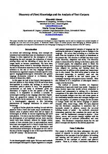
give an operator a semantic overview of a long video in a short period of time [6] and (v) Anomaly detection to highlight to an operator the most unusual events in a recording period [1], [2], [3]. So far, all of these tasks have generally been addressed within a single scene (single video captured by a static camera), or a group of adjacent scenes. Compared with single scene recordings, the multi-camera surveillance network (cameras distributed over different locations) is a more realistic scenario in surveillance applications and thus of more interest to end users. An example of a multi-camera surveillance network is given in Fig 1, where surveillance videos capture mostly traffic scenes with various layouts and motion patterns. In such a multi-scene context, new surveillance tasks arise. For behaviour profiling / scene understanding, human operators would like to see which scenes within the network are semantically similar to each other (e.g. similar scene layout and motion patterns), which activities are in common – and which are unique – across a group of scenes, and how activities group into behaviours. Here activity refers to a spatio-temporally compact motion pattern due to the action of a single or small group of objects (e.g. vehicles making a turn) and behaviour refers to the interaction between multiple activities within a short temporal segment (e.g. horizontal traffic flow with vehicles going east and west and making a turn). For query-by-example, searching for a specified example behaviour should be carried out not only within scene but also across multiple scenes. For behaviour classification, annotating training examples in every scene exhaustively is not scalable. However multi-scene modelling potentially addresses this by allowing labels to be propagated from one scene to another. For summarization, generating a summary video for multiple scenes by exploiting crossscene redundancy can provide the user who monitors a set of cameras with an overview of all the distinctive behaviours that have occurred in a set of scenes. Multi-scene summarisation can reduce the summary length and achieve higher compression than single-scene summarization. Combined with queryby-example (find more instances of a behaviour in a summary), a flexible exploration of scenes at multiple scales is available. Despite the clear potential benefits of exploiting multiscene surveillance, it can not be achieved with existing singlescene models [1], [2], [3], [4], [5]. These approaches learn an independent model for each scene and do not discover corresponding activities or behaviours across scenes even if they share the same semantic meaning. This makes any crossscene reasoning about activities or behaviours impossible. In order to synergistically exploit multiple scenes in surveillance, a multi-scene model with the following capabilities

IEEE TRANSACTIONS ON CIRCUITS AND SYSTEMS FOR VIDEO TECHNOLOGY

2

be discovered in order to exploit their similarity for cross-scene query-by-example and multi-scene summarization. Both common and unique activities should be preserved in this process to ensure the ability of discovering not only the commonality but also the distinctiveness between scenes.

Fig. 1: An example of multi-camera surveillance network with camera views distributed across different locations.

is required: (i) Learning an activity representation that can be shared across scenes; (ii) Model behaviours with the shared representation so they are comparable across scenes and (iii) Generalising surveillance tasks to the multi-scene case, including behaviour profiling/scene understanding, cross-scene query-by-example, cross-scene classification and multi-scene summarization. However this is intrinsically challenging for three reasons: 1) Computing Scene Relatedness Determining the relatedness of scenes is critical for multi-scene modelling because naive information sharing between insufficiently related scenes can easily result in ‘negative transfer’ [7], [8]. However, the relatedness of scenes is hard to estimate because the appearance of elements in a scene (e.g. buildings, road surface markings, etc.) is visually diverse, and strongly affected by camera view, making appearancebased similarity measurement unreliable. Similarity measurement based on motion is less prone to visual noise in surveillance applications. However most studies only focus on discovering the similarity in activity level [9], [8]. Thus how to measure scene-level relatedness is still an open question. 2) Selective sharing of information Large multi-camera surveillance networks covers various types of scenes. Some scenes are totally unrelated which means they convey different semantic meanings to a human. However, more subtly, even between similar scenes, there may be some activities in common and other activities that are unique to each. Learning a large universal model in this situation is prone to over-fitting due to the high model complexity. Hence a model that discovers (un)relatedness of scenes and selectively shares activities between them is necessary. 3) Constructing a shared representation Within related scenes, a shared representation needs to

To address these challenges we develop a new framework illustrated in Fig. 2. We first learn local representations for each scene separately. Then related scenes are discovered by clustering. A shared semantic representation is constructed to represent activities and behaviours within each group of related scenes. Specifically, we first represent each scene with a low-dimensional ‘semantic’ (rather than pixel level) representation through learning a fast unsupervised topic model for each1 . Using a topic-based representation allows us to reduce the impact of pixel-noise in discovering activity and scene similarity. We next group semantically related scenes into a scene cluster by exploiting the correspondence of activities between different scenes. Finally, scenes within each cluster are projected to a shared representational space by computing a shared activity topic basis (STB), shared among all scenes but also allowing each scene to have unique topics if supported by the data. Behaviours in each scene are represented with the learned STB. In addition to profiling for revealing the multi-scene activity structure across all scenes, we use this structured representation to support cross-scene query, label-propagation for classification and multi-scene summarization. Cross-scene query by example is enabled because within each cluster, the semantic representation is shared, so an example in one scene can retrieve related examples in every other scene in the cluster. Behavior classification/annotation in a new scene without annotations is supported because, once associated to a scene cluster, it can borrow the label-space and classifier from that cluster. Finally, we define a novel jointly multiscene approach to summarization that exploits the shared representation to compress redundancy both within and across scenes of each cluster. II. R ELATED W ORK Surveillance Scene Understanding Scene understanding is a wide area that is too broad to review here. However, some relevant studies to this work include those based on object tracking [3], [10], [11], [12], which model behaviours for example by Hidden Markov Model (HMM) [3], [10], Gaussian Process [12], clustering [13] and stochastic contextfree grammars [14] and those based on low-level feature statistics such as optical flow [15], [1], [2], [5] that often model behaviours by probabilistic topic model (PTM) [1], [2], [4]. The latter category of approaches are the most related to ours, as we also built upon PTMs. However, all of these studies operate within-scene rather than modelling globally distributed scenes and discovering shared activities. 1 Topics have previously been shown to robustly reveal semantic activities from cluttered scenes [1], [2].

IEEE TRANSACTIONS ON CIRCUITS AND SYSTEMS FOR VIDEO TECHNOLOGY

3

Cross-Scene Query by Example Cross-Scene Classification Multi-Scene Video Summarization

…

Fig. 2: An illustration of the proposed framework. Multi-Scene Understanding We make an explicit distinction to another line of work that discovers connections and correlations between multiple overlapping or non-overlapping scenes connected by a single camera network covering small areas [16], [17]. This is orthogonal to our area of interest, which is more similar to multi-task learning [7] - how to share information between multiple scenes some of which have semantic similarities, but do not necessarily concurrently surveil topologically connected zones. Fewer approaches have tried to exploit relatedness between scenes without a topological relationship [9], [8]. To recognize the same activity from another viewpoint, Khorkhar et al. [9] proposed a geometric transformation based method to align two events, represented as Gaussian mixtures, before computing their similarity. Xu et al. [8] used a trajectory-based event description and learned motion models from trajectories observed in a source domain. This model was then used for cross-domain classification and anomaly detection. In the context of static image (rather than dynamic scene) understanding [18], [19], studies have clustered images by appearance similarity. However, this does not apply directly to surveillance scenes because the background is no longer stationary nor uniform, e.g. building and road appearance are visually salient but can vary significantly between surveillance scenes at different locations. It is not reliable to relate surveillance scenes based on appearance - the important cue is activity instead. Video Query and Annotation Video query has always been an important issue in surveillance applications. A lot of work has been done on semantic retrieval [20], [1]. Hu et al. [20] used trajectories to learn an activity model and construct semantic indices for video databases. Wang et al. [1] represents video clips as topic profiles and measures similarity between query and candidate clips as relative entropy. Retrieved clips are sorted according to the distance to the query. However none of these techniques take a multi-scene scenario into consideration, where query examples are selected in one scene and candidate clips can be retrieved from other scenes at different locations. Related to video query, video behaviour annotation/classification has been addressed in the literature [1], also in terms of video segmentation [21]. However, these approaches are typically domain/scene-specific, which means that each scene needs extensive annotation of training data; where ideally labels should instead be borrowed from semantically related scenes. Although a recent study

[9] recognised events across scenes at the activity level, scene level behaviour classification, and dealing with a heterogeneous database of scenes is still an open problem. Video Summarization Video summarization has received much attention in the literature in recent years due to the need to digest large quantities of video for efficient review by users. A review can be found in [22]. There are a variety of approaches to summarization, varying both in how the summary is represented/composed, and how the task is formalised in terms of what type of redundancy should be compressed. Summaries have been composed by: static keyframes that represent the summary as a collection of selected key-frames [23], dynamic skimming which composes a summary based on a collection of selected clips, and more recently synopsis. Synopsis [24], [6] temporally re-orders (spatially non-overlapping) activities from the original video into a temporally compact summary video by shifting activity tubes temporally so they occur more densely. The objective of summarization can be formalised in various ways: to show all foreground activity in the shortest time [24], to minimise the reconstruction error between the summary and the original video, to show at least one example of every typical behaviour, or more abstractly to achieve the highest rating in a user study [23]. As the number of scenes grows, multi-view summarization becomes increasingly important to help operators monitor activities in numerous scenes. However, multi-view summarization is much less studied compared to that of single view. Lou et al. [25] adopted multi-view video coding to deal with multi-view video compression, but did not tackle the more challenging compression of semantic redundancy. Fu et al. [26] addressed generating concise multi-view video summaries by multi-objective optimisation for generating representative summary clips. Recently, De Leo et al. [27] proposed a multicamera video summarization framework which summarizes at the level of activity motif [28]. Due to the severe occlusion, far-field of view and high density activities in surveillance videos, none of the existing techniques solve the problem of distributed multi-scene surveillance video summarization. In this paper, we pursue video summarization from the perspective of selecting the smallest set of representative video clips that still have good coverage of all the behaviours in the scene(s). Such multi-scene summarization compresses redundancy across as well as within scenes. This corresponds to an application scenario where the user tasked with monitoring a set of cameras wants an overview of all the behaviours

IEEE TRANSACTIONS ON CIRCUITS AND SYSTEMS FOR VIDEO TECHNOLOGY

that occurred in a set of video streams during a recording period regardless the source of the video recordings, which typically come from different locations. This perspective on summarization is attractive because it makes sense of video content indepedent of location and local context. This offers a more holistic conceptual summarization in a global context as compared to summarization as visualisation of a single scene in a local context such as video synopsis. Interestingly, combined with our query-by-example, we can take a behaviour of interest shown in the summary as query to search for similar behaviours in other scenes. Thus the framework presents both compact multi-scene summarization and a finer scene-specific zoom-in, capable of compressing semantically equivalent examples no matter what scene they occur in. Our Contributions A system based on our framework can answer questions such as ‘show me which scenes are similar to this?’ (scene clustering), ‘show me which activities are in common and which are distinct between these scenes’ (multi-scene profiling) ‘show me all the distinct behaviours in this group of scenes’ (multi-scene summarization), ‘show me other clips from any scene that are similar to this nominated example’ (cross-scene query), ‘annotate this newly provided scene with no-labels’ (cross-scene classification). Specifically, we make the following key contributions: 1) Introducing the novel and challenging problems of joint multi-scene modelling and analysis. 2) Developing a framework to solve the proposed problem by discovering similarity between activities and scenes, clustering scenes based on semantic similarity and learning a shared representation within scene clusters. 3) We show how to exploit this novel structured multiscene model for practical yet challenging tasks of crossscene query-by-example and behaviour annotation. 4) We further exploit this model to achieve multi-scene video summarization, achieving compression beyond standard single-scene approaches. 5) We introduce a large multi-scene surveillance dataset containing 27 distinct views from distributed locations to encourage further investigation into realistic multiscene visual surveillance applications.

III. L EARNING L OCAL S CENE ACTIVITIES Given a set of surveillance scenes we first learn local activities in each individual scene using Latent Dirichlet Allocation (LDA) [29]. Although there are more sophisticated singlescene models [1], [2], [4], we use LDA because it is the simplest, most robust, most generally applicable to a wide variety of scene types, and the fastest for learning on large scale multi-scene data. However, it could easily be replaced by more elaborate topic models (e.g. HDP [1]). LDA generates a set of topics to explain each scene. Topics are usually spatially and temporally constrained sub-volumes reflecting the activity of a single or small group of objects. Following [1], [2], we use activities to refer to topics and behaviours to refer to scenelevel state defined by the coordinated activities of all scene participants.

4

A. Video Clip Representation We follow the general approach [1] to construct visual features for topic models. For each video out of an M scene dataset we first divide the video frame into Na × Nb cells with each cell covering H × H pixels. Within each cell we compute optical flow [30], taking the mean flow as the motion vector in that cell. Then we quantize motion vector into Nm fixed directions. Note, stationary foreground objects can be readily added as another cell state as described in [2], [31]. Therefore a codebook V of size Nv = Na × Nb × Nm is generated by mapping motion vectors to discrete visual words d (from 1 to Nv ). Nd visual documents X = {xj }N j=1 are then constructed by segmenting the video into non-overlapping Nj has Nj clips of fixed length, where each clip xj = {xij }i=1 visual words xij . Clip and document are used interchangeably here with both indicating visual words accumulated in a temporal segment. B. Learning Local Activities with Topic Model Learning LDA for scene s discovers the dynamic ‘appearance’ of k = 1 . . . K typical topics/activities2 (multinomial parameter βks ), and explains each visual word xsij in each clip s xsj by a latent topic yij specifying which activity generated s it, as shown in Fig. 3. The topic selection yij is drawn from multinomial mixture of topics parametrized by θjs which is further governed by a Dirchelet distribution with parameter αs . In scene s the joint probability of Nd visual documents s s Nd d Xs = {xsj }N j=1 , topic selection Y = {yj }j=1 and topic s s Nd mixture θ = {θj }j=1 given hyperparameters αs and β s is: p(θ s , Ys , Xs | αs , β s ) =

Nd Y

p(θjs | αs )·

j=1 Nj Y

s p(yij

|

θj )p(xsij

(1) |

s yij , βs )

i=1

𝜷𝑠 𝜶𝑠

𝜽𝑗𝑠

𝑦𝑖𝑗𝑠

Type equation here.

𝑠 𝑥𝑖𝑗 i=1…Nj

j=1….Nd s=1….M

Fig. 3: Graphical model for Latent Dirichlet Allocation. 1) Model Inference: Exact inference in LDA is intractable due to the coupling between θ and β [29]. Variational inference approximates a lower bound of log likelihood by introducing variational parameters γ and φ. Dirichlet parameter γj is a clip-level topic profile and specifies the mixture ratio of each activity βk in a clip xj . Thus, each video clip is 2 In text analysis, a topic refers to a group of co-occurring words in a document. Activity refers to a motion pattern, which defines the group of co-occurring visual words in a video clip. They are used interchangeably in the following text.

IEEE TRANSACTIONS ON CIRCUITS AND SYSTEMS FOR VIDEO TECHNOLOGY

represented as a mixture of activities (γj ). The variational EM procedure for LDA is given in Algorithm 1 where 1(·) is an indicator function and Ψ(·) is the first derivative of the log Γ function. For efficiency, we apply the sparse updates identified in [32] for an order of magnitude speed increase. Algorithm 1 Topic model learning for a single scene initialize αk = 1 initialize β = random(Nv , K) initialize φijk = 1/K repeat E-Step: for j = 1 → Nd do for k = 1 → KP do Nj γjk = αk + i=1 φijk for i = 1 → Nj do φijk = βxij k exp(Ψ(γjk )) end for end for end for M-Step: for v = 1 → Nv do for k = 1P → KP do Nj Nd βvk = j=1 i=1 φijk 1(xij = v) end for end for until Converge After learning all s = 1 . . . M scenes, every clip xsj is now represented as a topic profile γjs ; and each scene is now represented by its constituent activities βks (Fig. 4). IV. M ULTI -L AYER ACTIVITY AND S CENE C LUSTERING We next address how to discover related scenes and learn shared topics/activities across scenes. This multi-layer process is illustrated in Fig. 5 for two typical clusters 3 & 7: At the scene level we group related scenes according to activity correspondence (Section IV-A); within each scene cluster we further compute a shared activity topic basis so that all activities within that cluster are expressed in terms of the same set of topics (Section IV-B). A. Scene Level Clustering In order to group related scenes, we first need to define a relatedness metric. Related scenes should have more common activities so that the model learned from them is compact. So we assume the scenes with semantically similar activities are more likely to be mutually related. We thus define the relatedness between two (aligned) scenes a and b, by the correspondence of their semantic activities. a) Alignment: Comparing scenes directly suffers from cross-scene variance due to view angle. To reduce this crossscene variance we first align two scenes with a geometrical transformation including scaling ts and translation [tx , ty ]. Although this is not a strong transform it is valid in the typical case that a camera is installed upright, and with surveillance cameras there are classic views which can be simply aligned

5

by scaling and translation. To achieve this, we first denote the transform matrix for normalizing visual words in each scene a and b to the origin as Tanorm and Tbnorm defined as Eq. (2). Scaling (tas ) and translation (tx , ty ) parameters are estimated by Eq. (3). a  ts 0 tax Tanorm =  0 tas tay  (2) 0 0 1

center =

Nj Nd X X 1 xa , Nd · Nj j=1 i=1 ij

Nd · Nj , tas = PN PNj d a i=1 kxij − centerk2 j=1  a tx = −tas · center tay

(3)

Two scenes can thus be aligned by transforming data from a a to b via Ta2b = Tb−1 norm · Tnorm . We then denote kth topic a in scene a as βk . So any topic k in a can be aligned for comparison with those in b by Ta2b . We denote the topic transformation procedure as β 0 = H(β; T). This transformation is applied to topics in a similar way as image transform. That is, given that β is a Na × Nb × Nm matrix and a transform matrix T is defined as Eq (2), we first estimate the size Na0 ×Nb0 ×Nm of transformed topic β 0 by Na0 = Na × ts and Nb0 = Nb × ts . To obtain the value for each element/pixel of β 0 (x0 , y 0 , d0 ), we trace back to the position [x, y, d] in the original topic β. If we only consider scaling and translation, direction d is then unchanged throughout the procedure i.e. d0 = d. Therefore, x and y are determined by:     x y 1 = x0 y 0 1 · (T−1 )T (4) In most cases, x and y are not discrete values because of the matrix multiplication. In order to obtain the value for β(x0 , y 0 , d0 ), we perform interpolation, i.e. we use the values of adjacent pixels surrounding [x, y, d] to determine the value of β(x0 , y 0 , d0 ). This interpolation is only related to spatial values in a single layer, i.e. d is fixed, and we only use the adjacent pixels by varying x and y. A number of standard interpolation techniques can be used for this task including linear, bilinear and bicubic interpolations and we use bicubic interpolation here. After interpolation, we compute the exact value for each element/pixel β(x0 , y 0 , d0 ). Due to that this transformation involves translation, the transformed topic β 0 may extend out of the topic boundary, a Na × Nb rectangle, defined by the original topic β. To ensure all topics being comparable with the same codebook size, we only keep the part of β 0 that lies within the Na ×Nb rectangle defined by the original topic β. After the above procedure, the transformed topic β 0 has the same size as the original β, Na × Nb × Nm . Finally, we normalise the transformed topic β 0 to obtain a multinomial distribution, as follows:

β0 =

P

P

β0 P

x=1···Na y=1···Nb d=1···Nm

β 0 (x,y,d)

(5)

IEEE TRANSACTIONS ON CIRCUITS AND SYSTEMS FOR VIDEO TECHNOLOGY

6

Fig. 4: Locally learned activities/topics in an example scene. The optical flow is quantized into Nm = 8 directions as shown in the colorwheel. I.

……

Surveillance video scenes s=1…S

II.

……

Scene level Clusters c=1…C

Local topics for each scene s { βks }Kk =1

III.

……

Activity Clusters t=1…T

STB topics stb { βkstb }Kk =1

……

Fig. 5: An illustration of multi-layer clustering of scenes and activities. Block I (Top) illustrates the original surveillance video scenes. Block II (middle) illustrates (i) related scenes are grouped into clusters (indicated by green dashed boxes) and (ii) the local topics/activities learned in each scene. Block III (bottom) illustrates (i) local topics are furthered grouped into activity clusters (color lines indicate some examples) and (ii) activity clusters are merged to construct a shared activity topic basis (STB). b) Affinity and clustering: Given the scene alignment above, we define the relatedness between scenes a and b by the percentage of corresponding topic pairs. More specifically, a b given K a local topics {βkaa }K ka =1 in scene a and K local b Kb topics {βkb }kb =1 in scene b, the distance between topic βkaa and topic βkb b is defined as DKL in Eq. (6): 1 b b2a = (KL(βka2b || βkaa )) a || βk b ) + KL(βk b 2 ! Nv 1 X βkaa v a b a KL(βka || βkb ) = β a · log Nv v=1 k v βkb b v

binarized. Topic pairs with distance less than a threshold are counted as inliers, defined by: N umInlier =

X

1(min(DKL (βkaa , βkb b )) < τ ) kb

ka

+

X

1(min (DKL (βkb b , βkaa )) < τ ) a

kb

DKL (βkaa , βkb b )

(6)

Given a threshold τ the similarity between two topics can be

(7)

k

where 1(·) is the indicator function. The final relatedness measure D(a, b) between scenes a and b is the percentage of inlier topic pairs: D(a, b) =

N umInlier Ka + Kb

(8)

IEEE TRANSACTIONS ON CIRCUITS AND SYSTEMS FOR VIDEO TECHNOLOGY

Since Eqs. 6 and 7 are symmetric, Eq. 8 is as well. Given this relatedness measure, every scene pair is compared to generate an affinity matrix, and self-tuning spectral clustering [33] is used to group scenes into c = 1 . . . C semantically similar scene-level clusters. (See Fig. 5 II for an example). B. Learning A Shared Activity Topic Basis Scenes clustered according to Section IV-A are semantically similar, however the representation in each is still distinct. We next show how to establish a shared representation for every scene in a particular cluster. We denote the set of scenes in a cluster as C. We first choose the scene with the lowest distance to all other scenes in the cluster as the reference scene/coordinate sref . Activities in all scenes s ∈ C can be projected to the reference coordinates via transform Ts2sref as stated in Eq. (9). ∀s ∈ C, ∀k = 1 . . . K : β˜ks = H(βks ; Ts2sref )

(9)

Once every topic is in the same coordinate system, we create ˜s }s∈C usan affinity matrix for all the transformed topics {β k ing the symmetrical Kullbeck-Leibler Divergence as distance metric (Eq. (6)). Hierarchical clustering is then applied to stb group the projected activities into K stb clusters {Tk }K k=1 . (Tk denotes the set of activities in a cluster k). The result is that semantically corresponding activities across scenes are now grouped into the same cluster. We then take the mean of activities in each activity cluster Tk as one shared activity topic βkstb as in Eq. (10). An alternative to this approach is to re-learn topics from the concatenation of visual words of all the scenes in a single cluster. However, this ‘Learningfrom-Scratch’ strategy prevents explicitly identifying shared and unique topics across scenes. Because the trace of local topics from individual scenes to STB is lost. In contrast, our framework reveals how scenes are similar or different. ∀k = 1 . . . K stb : βkstb =

1 | Tk |

X

˜ks00 β

(10)

7

and classification can be achieved. Cross-scene query Activity-based query by example aims at retrieving semantically similar clips to a given query clip. In the cross-scene context, the pool of potential clips to be searched for retrieval includes clips from every camera in the network. Within a scene cluster C, we segment each video s into j = 1 . . . Nd short clips (Section III-A). We represent stb defined the jth video clip in scene s as topic profile γjs stb on STB βk . A query clip q, represented by STB profile stb γqs can now be directly compared against all other clips stb in the cluster {γjs 0 }j,s0 ∈C using L2 distance. In this way, cross-scene query-by-example is achieved by sorting all clips in the cluster according to distance to the query. Cross-scene classification Given an existing annotated database of scenes modelled with our multi-layer framework, classification in a new scene s∗ can now be achieved without further annotation. First s∗ is associated to a cluster c∗ (Section IV-A). Although s∗ has no annotation, this reveals a set of semantically corresponding existing scenes from which annotation can meaningfully be borrowed. Classification can thus be achieved by any classifier, using all other scenes/clips and labels from cluster c∗ as the labeled training set. It should be noted that our cross-scene classification differs from [34], [35] in: (1) We train on a set of source scenes before testing on a held-out scene rather than one source to one test scene. The conventional 1-1 approach requires implicitly the source and target scene to be relevant which must be manually identified. Our model is able to group relevant scenes automatically without requiring the user to know this as a priori. (2) Our model works in a transductive [7] manner. That is, it looks at target scene data during scene clustering, but without looking at the target data label. This weak assumption is more desirable in practice because surveillance video data is often easy to collect but without any labelling, whilst the effort required for labelling is the bottleneck.

k0 ,s0 ∈Tk stb

We denote the set of shared activity topics {βkstb }K k=1 learned for the cluster as the shared activity topic basis (STB). The resulting STB captures both common and unique activities in every scene member. See Fig. 5III for an example. We can now represent the behaviours in every scene as STB profiles: by projecting the STB back to each scene and re-computing stb the topic profile γjstb defined now on {βkstb }K k=1 ; in contrast to the original scene-specific representation (γjs , defined in terms of {βks }K k=1 ). That is, re-running Algorithm 1, but with β fixed to the STB values obtained from Eq. (10). An example of behaviour profiling on STB is illustrated in Fig. 6. Visual words accumulated within a clip are profiled according to the STB. Thus each behaviour can be treated as a weighted mixture of multiple activities. V. C ROSS -S CENE Q UERY BY E XAMPLE AND C LASSIFICATION Given the structured multi-scene model introduced in the previous section, we can now describe how cross-scene query

VI. M ULTI -S CENE S UMMARIZATION In this section we present a multi-scene video summarization algorithm that exploits the structure learned in Section IV to compress cross-scene redundancy. All clips are represented by their profile on STB. The general objective of multi-scene summarization is to generate a video skim with at least one example of each distinct behaviour in the shortest possible summary. We generate independent summaries for each scene cluster (since different scene clusters are semantically dissimilar), and multi-scene summaries within each cluster (since scenes within a cluster are semantically similar). K-center summaries: The multi-scene summary video is of configurable length Nsum . Longer videos will show more distinct behaviours or more within-class variability of each behaviour. We compose the summary Σ of Nsum clips {γjstb }, j ∈ Σ drawn from all scenes in the cluster. The obstb jective is that all clips in the cluster {γjs }j,s∈C should be

IEEE TRANSACTIONS ON CIRCUITS AND SYSTEMS FOR VIDEO TECHNOLOGY

8

Video Clip (Behaviour) Profiled by STB

STB Profile γ as Bar Chart

STB Topics 1-20

Fig. 6: An illustration of behaviour profiling on STB. In the left block, visual words are profiled by STB and plotted as coloured dots. Notice that colors here indicate visual words belonging to individual activities in STB instead of motion direction. Profiling γ is also given as bar chart where x axis indexes STB activities. The right block illustrates the STB activities where color patches indicate distribution of motion vectors. near to at least one clip in the summary (i.e., the summary is representative). Formally, this objective is to find the summary set Σ that minimizes the cost J in Eq. (11) where Dγ is the L2 distance:  
stb stb J = max max D γ , γ (11) 0 γ j js 0 j,s∈C

j ∈Σ

This is essentially a k-center problem [36]. Since it is intractable to enumerate all combinations/potential summaries Σ, we adopt the 2-approximation algorithm [37] to this optimization. The resulting K = Nsum centers identify the summary clips. VII. E XPERIMENTS Dataset: We collected 25 real traffic surveillance videos from publicly accessible online web-cameras in Budapest, Hungary. These videos are combined with two surveillance video datasets Junction and Roundabout [15] for a total of 27 videos. Sample frames for each scene are illustrated in Fig. 7(a). We trim each video to 18 000 frames in 10fps, of which 9 000 are used to learn the model and the remaining 9 000 frames are used for testing (query, classification and summarization). For activity learning we segment each training video into 25 frame clips, so 360 clips are generated for each scene. For both query and summarization applications, we segment test videos into clips with 80 frames, so 112 clips for query and summarization are generated from each scene. Thus, we have three types of video clips: (1) Clips for unsupervised training of LDA, (2) clips for training crossscene classification, retrieval and multi-scene summarization, (Semantic Training Clips), (3) clips for testing cross-the same tasks (Semantic Testing Clips). LDA clips are shorter (25 frames) to facilitate learning more cleanly segmented activities. Semantic clips are longer (80 frames) as a more humanscale user-friendly unit for visualisation and annotation.

Learning Activities: We computed optical flow [30] for all videos by quantizing the scenes with 5 × 5 pixel cells and 8 directions. Local activities are learned from each video independently using LDA with K = 15 activities per scene. Behaviour Annotation: Behaviour is a clip-level semantic tag defining the overall scene-activity. Due to the semantic gap between behaviours in the video clip and (potentially task dependent) human interpretation, it is difficult to give video a concise and consistent semantic label (in contrast to human action [34] and event [9] recognition). Instead of annotating each video clip explicitly, we give a set of binary activity tags (each representing the action of some objects within the scene) to each video clip as shown in Table I. All the tags associated with vehicles have a sparse or dense option. When there are less than three vehicles travelling in a clip, it is labelled as sparse, otherwise dense. Each unique combination of activities that exists in the labelled clips then defines a unique scenelevel behaviour category. We explore this through multiple sets of annotations: an original annotation with 19 distinct tags, and subsequent coarser label sets derived by merge scheme 1 with 13 distinct tags and merge scheme 2 with 10 distinct tags. The activity tags are given in Table I. We exhaustively annotate video clips in two example scene clusters (3 and 7 as shown in Fig. 7). Across the two clusters, there are 6 scenes with 112 clips per scene annotated (672 clips in total). In the original annotation case, there are 111 total behaviours identified. The distribution of behaviours are illustrated in Fig. 8(a). However this number is more than necessary in terms of limited distinctiveness of the numerous entailed behaviours. By merging some activity annotations we generate 59 or 31 (Merge Scheme 1 or 2 in Table I) unique behaviours. It should be noted that the frequency of behaviours is rather imbalanced, as indicated by all the subfigures of Fig. 8. There is also very limited overlap of behaviours between scene clusters 3

IEEE TRANSACTIONS ON CIRCUITS AND SYSTEMS FOR VIDEO TECHNOLOGY

Scene 1

Scene 2

Cluster 1

Scene 3

Cluster 1

Scene 10

Cluster 1

Scene 11

Cluster 3

Cluster 7

Scene 15

Cluster 5

Cluster 5

Scene 23

Scene 22

Cluster 8

Cluster 2

Scene 14

Cluster 4

Scene 21

Cluster 8

Cluster 2

Scene 13

Cluster 4

Scene 20

Scene 6

Scene 5

Cluster 1

Scene 12

Cluster 4

Scene 19

Scene 4

9

Cluster 8

Scene 24

Cluster 9

Cluster 9

Scene 7

Cluster 3

Scene 8

Cluster 3

Scene 16

Cluster 6

Scene 17

Cluster 6

Scene 25

Cluster 9

Scene 26

Cluster 10

Scene 9

Cluster 3

Scene 18

Cluster 7

Scene 27

Cluster 11

Frequency of Behaviours

Fig. 7: Example frames for our multi-surveillance video dataset with each scene assigned a reference number on top of the frame. The color of bounding box and text in the bottom left indicates assigned cluster. TABLE I: Original annotation ontology and two merging 80 Scene Cluster 3 Scene Cluster 7 schemes give multiple granularities of annotation. 60

40

20

0

10

20

30

40

50

60 Behaviours

70

80

90

100

110

(a) Behaviour frequency: original annotation 200

Scene Cluster 3 Scene Cluster 7

Frequency of Behaviours

Frequency of Behaviours

150

100

50

0

10

20

30 Behaviours

40

50

(b) Behaviour frequency: merge scheme 1

Scene Cluster 3 Scene Cluster 7

150

100

50

0

10 20 Behaviours

30

(c) Behaviour frequency: merge scheme 2

Fig. 8: Frequencies of behaviours of each category. (a), (b) and (c) illustrate the frequency of behaviours when varying the labelling criteria.

No.

Original Annotation

1 2 3 4 5 6 7 8 9 10 11 12 13 14 15 16 17 18 19

Vehicle Left Sparse Vehicle Left Dense Vehicle Right Sparse Vehicle Right Dense Vehicle Up Sparse Vehicle Up Dense Vehicle Down Sparse Vehicle Down Dense Vehicle Southeast Sparse Vehicle Southeast Dense Vehicle Northwest Sparse Vehicle Northwest Dense Vehicle Up2Right Turn Vehicle Left2Up Turn Vehicle Up2Left Turn Tram Up Tram Down Pedestrian Horizontal Pedestrian Vertical

Merge Scheme 1 Vehicle Left

Merge Scheme 2 Vehicle Horizontal

Vehicle Right Vehicle Up

Vehicle Vertical

Vehicle Down Vehicle Southeast

Vehicle SE& NW

Vehicle Northwest Vehicle Up2Right Turn Vehicle Left2Up Turn Vehicle Up2Left Turn Tram Up Tram Down Pedestrian Horizontal Pedestrian Vertical

Vehicle Up2Right Turn Vehicle Left2Up Turn Vehicle Up2Left Turn Tram Up Tram Down Pedestrian Horizontal Pedestrian Vertical

and unique views are separated into their own cluster (e.g. Cluster 11).

and 7. To assess annotation consistency and bias, we invited eight independent annotators to annotate all the video clips separately. We observe that the additional annotations are fairly consistent with the original annotation: with more than 80% agreement (Hamming distance) between the additional and the original annotations. Detailed analysis of these additional annotations are given in the supplementary material.

Learning A Shared Activity Topic Representation: Within each scene cluster we unify the representation by computing a shared activity topic basis. We automatically set the number of shared activities K stb in each scene cluster with Ns scenes as K stb = coef f × Ns where coef f is set to 5. The discovered basis from an example cluster (Scene Cluster 3 shown in Fig.7) with 4 scene members is illustrated in Fig. 9. This figure reveals both activities unique to each scene (Topics 115) and activities common among multiple scenes (Topic 1620). Thus some shared activity topics are composed of single local/original topics, and others of multiple local topics.

A. Multi-Layer Scene Clustering

B. Cross-Scene Query by Example and Classification

Scene Level Clustering: We first group the scenes into semantically similar clusters by spectral clustering. The similarity measurement between scenes is the number of corresponding activities, as defined in Section IV-A. The self-tuning spectral clustering automatically determines the appropriate number of clusters which, in the case of our 27-scene dataset, is 11 clusters. Fig. 7 shows the results, in which semantically similar scenes are indeed grouped (e.g. Camera towards one direction at road junctions in Cluster 3),

In this section we evaluate the ability of our framework to support two tasks: cross-scene query by example; and cross-scene behaviour classification. We compare our Scene Cluster Model (SCM) with a baseline Flat Model (FM). Our Scene Cluster Model first group scenes into scene clusters according to their relatedness and learns STB for every scene cluster. Video clips in each scene cluster are thus represented as topic profiles on the STB of the scene cluster. As with our model, a Flat Model first learns a local

IEEE TRANSACTIONS ON CIRCUITS AND SYSTEMS FOR VIDEO TECHNOLOGY

10

Composition of Shared Activity Topics in Scene Cluster 3 Shared Activity Topics 1-5

Original Topics 1-5

Original Topics 6-10

Shared Activity Topics 6-10

Original Shared Topics 11-15 Activity Topics 11-15

Shared Activity Topics 16-18

Original Topics 16-18

Shared Activity Topics 19-20

Original Topics 18-20

Fig. 9: Example STB learned from Scene Cluster 3. Shared activity topics may be composed of one or more local/original topics. Original topics are overlaid on background frame. Color patches indicate distribution of motion vectors for a single activity. 0.16

MAP SCM Merge Sch 2 MAP FM Merge Sch 2 MAP SCM Merge Sch 1 MAP FM Merge Sch 1

0.14 0.12

Query Clips

Retrieved Clips from Other Scenes

MAP

0.1 0.08 0.06 0.04 0.02 0 0

20

40

60

80

100

120

140

160

180

200

Query T number

Fig. 10: Query by example MAP with different number of retrievals topic model per scene, however it then learns a single STB from all labelled scenes (6 scenes from 2 clusters) without scene level clustering, instead of one STB per-cluster. The only difference between SCM and FM is the absence of scene-level clustering in FM. Note that the Flat Model is a special case of our Scene Cluster Model with 1 scene-level cluster. Moreover, the individual scenes are also a special case of our Scene Cluster Model with one cluster per scene. Query by Example Evaluation: To quantitatively evaluate query by example, we exhaustively take each scene and each clip in turn as the query, and all other scenes are considered as the pool. All clips in the pool are ranked according to similarity (L2 distance on STB profile) to the query. Performance is evaluated according to how many clips with the same behaviour as the query clip are in the top T responses. We retrieve the best T = 1 · · · 200 clips and calculate the Average Precision of each category for each T . MAP is computed by taking the mean value of Average Precision over all categories. The MAP curve by the top T responses to a query for both Scene Cluster Model (SCM) and Flat Model (FM) and Merge Scheme 1 and 2 are plotted in Fig. 10. It is evident that for both Merge Scheme 1 and 2, the proposed scene cluster model (SCM) performs consistently better than the Flat Model (FM) regardless of number of top retrievals T. This is because

Fig. 11: Examples of cross-scene query by example. The first column gives 6 query clips randomly chosen from 6 scenes. The right image matrix illustrates the retrieved clips from the remaining 5 scenes, sorted by distance to query from left to right in the matrix. Color patches overlaid on the background indicates the visual words accumulated within a video clip.

in the Scene Cluster Model, the STB learned from this set of scenes are highly relevant to each scene in the cluster. In contrast, the Flat Model learns a single STB for all scenes making the STB less relevant to each individual scene, hence less informative as a representation for retrieval. Qualitative results are also given in Fig. 11 by presenting 6 randomly chosen queries and their retrieved clips. Different types of behaviours are covered by query clips and most retrieved clips are semantically similar to query clips. The only exception is in the 3rd row where the query clip indicates traffic going east and turning from left to up. This is because there is no corresponding behaviour in the other scenes.

IEEE TRANSACTIONS ON CIRCUITS AND SYSTEMS FOR VIDEO TECHNOLOGY

Classification Evaluation: In this experiment we quantitatively evaluate classification performance where the test scene has no labels. Successful classification thus depends correctly finding semantically related scenes and appropriately transferring labels from them (Section V). We perform leave one scene out evaluation by holding out one scene as the unlabelled testing set, and predicting the labels for the test set clips using the labels in remaining scenes using the KNN classifier. The KNN K parameter is determined by cross validating among the remaining scenes. Classification performance is evaluated by the accuracy for each category of behaviour, averaged over all held out scenes. TABLE II: Cross-scene classification accuracy with 31 and 59 categories for both Scene Cluster Model (SCM) and Flat Model (FM). Category Scene 1 Scene 2 Scene 3 Scene 4 Scene 5 Scene 6 Average

31

11

TABLE III: Summarization schemes for Condition WC Summarization Method Random Single-Scene Graph

Single-Scene Kcenter Multi-Scene Graph

Multi-Scene Kcenter

Description This lower-bound picks clips randomly from multiple scenes to compose the summary The overall summary is a concatenation of independent summaries for each video by doing recursive Normalized cut [38] on a graph constructed by taking each video clip as vertices and L2 distance between topic profile γ of each clip as edges. Here each video clip is represented by scene-specific local topics. This corresponds to [39], but without temporal graph. Similar to Single-Scene Graph method, but using Kcenter algorithm in Eq. (11) for summarization instead of Normalized Cut. This model learns a STB to represent video clips from all scenes with STB profile. Then Normalized Cut is applied to cluster clips and find multi-scene summaries. Our full model builds a STB from all scenes within a cluster, then uses the Kcenter algorithm to select summary clips from all scenes.

59

SCM

FM

SCM

FM

55.36% 27.68% 49.11% 54.46% 30.36% 38.39% 42.56%

50.89% 39.29% 41.96% 46.43% 26.79% 25.00% 38.39%

42.86% 18.75% 39.29% 37.50% 17.86% 20.54% 29.47%

40.18% 16.96% 37.50% 36.61% 17.86% 12.50% 26.94%

From Table II we observe that at either granularity of annotation (59 or 31 categories), our Scene Cluster Model outperforms the Flat Model on average. This shows that again in order to borrow labels from other scenes for cross-scene classification, it is important to select relevant sources, which we achieve via scene clustering. The Flat Model is easily confused by the wider variety of scenes to borrow labels from, while our Scene Cluster Model structures similar scenes and borrows labels from only semantic related scenes to avoid ‘negative transfer’ [7], [8].

Model Learns a single STB from all scenes available without discrimination while Scene Cluster Model learns a STB per scene cluster. Specifically, we compare the summarization schemes in Table IV. TABLE IV: Summarization schemes for Condition AC Summarization Method Random Flat Multi-Scene User Attention

Flat Multi-Scene Graph Flat Multi-Scene Kcenter Scene Cluster Multi-Scene Kcenter

Description This picks clips randomly from multiple scenes to compose the summary Leverages the magnitude, spatial and temporal phase of optical flow vectors to index videos. This is the visual attention measurement of ([40], Eq. (6)). We tested the model on a combined video by concatenating each individual video. This model uses Normalized Cut [38] to cluster all video clips represented as single STB profiles. This is similar to [39]. Same as Flat Multi-Scene Graph, but using Kcenter to select summary clips. Our full model clusters the scenes, learns STBs on each scene cluster, followed by Kcenter to summaries within each scene cluster

C. Multi-Scene Summarization In the final experiment, we evaluate our multi-scene summarization model against a variety of alternatives. We consider two conditions: In the first, we consider multi-scene summarization within a scene cluster (Condition WC); in the second we consider unconstrained multi-scene summarization including videos spanning multiple scene clusters (Condition AC). Condition: Within-cluster summarization (WC) In this experiment we focus on the comparison between Multi-Scene Model and Single-Scene Model given various summarization algorithms. The Multi-Scene Model represents all video clips from different scenes within a cluster with a single STB learned from the scene cluster while the Single-Scene Model represents each video with scene specific activities and the overall summary is the mere concatenation of summaries from each scene. Specifically, we compare the summarization methods listed in Table III. Condition: Across-cluster summarization (AC) In this experiment, analogous to query and classification, we focus on the comparison between Flat Model and Scene Cluster Model given different summarization algorithms. The Flat

Settings: To systematically evaluate summarization performance, we vary the length of the requested summary. In Condition WC the summary varies from 8 to 120 clips (64seconds to 16mins) out of overall 448 video clips (59.7mins) in Scene Cluster 3 (as shown in Fig. 7(a)) and 224 video clips (29.9mins) in Scene Cluster 7. In Condition AC the summary varies from 6 to 120 clips (48seconds to 16mins) out of 672 video clips (89.7mins) total which is a combination of Scene Cluster 3 and 7. All video clips for summarization are represented as topic profile γ. Recall that each local scene is learned with K = 15 topics and scene clusters with Ns scenes are learned with K = coef f × Ns topics where coef f is set to 5 here. For fair comparison, flat model baselines are learned with the sum of the number of topics for each cluster. Summarization Evaluation The performance is evaluated by the coverage of identified behaviours in the summary, averaged over 50 independent runs. Fig. 12(a) and (b) show the results for multi-scene summarization within two example clusters (Condition WC). Clearly our Multi-Scene Kcenter algorithm (red) outperforms the baselines: both Graph Method alternative (purple), and single-scene alternatives (dashed line). The

IEEE TRANSACTIONS ON CIRCUITS AND SYSTEMS FOR VIDEO TECHNOLOGY

performance margin is greater between multi-scene and singlescene models for the first cluster because there are four scenes here, so greater opportunity to exploit inter-scene redundancy. This validates the effectiveness of jointly exploiting multiplescenes for summarization. Fig. 12(c) shows the result for multi-scene summarization across both clusters (Condition AC): our Scene Cluster Model builds one summary for each cluster to exploit the expected greater volume of within-cluster redundancy. In contrast, the Flat Model builds one single summary, but for a much more diverse group of data, and the single-scene models have no across-cluster redundancy to exploit. Even in the flat case, our Kcenter model (in green) still outperforms all other alternatives (purple and magenta). It is also worth noting that the user attention model degenerates severely on our dataset due to the inability to extract semantic meaning from videos where pure motion strength is not informative enough to distinguish semantic behaviours. Qualitative results for multi-scene summarization are presented in supplementary material.

Coverage of Behaviours (%)

90 80 70 60 50 40 Random Single−Scene Graph Method Single−Scene Kcenter Multi−Scene Graph Method Multi−Scene Kcenter

30 20 10 0

20

40

60 Summary Length (clips)

80

100

120

(a) Condition WC: Scene Cluster 3 (4 scenes total)

Coverage of Behaviours (%)

100 90 80 70 60 50 Random Single−Scene Graph Method Single−Scene Kcenter Multi−Scene Graph Method Multi−Scene Kcenter

40 30 20 0

20

40

60 Summary Length (clips)

80

100

120

(b) Condition WC: Scene Cluster 7 (2 scenes total)

Coverage of Behaviours (%)

80 70 60 50 40 30 20

Random Flat Multi−Scene User Attention Flat Multi−Scene Graph Method Flat Multi−Scene Kcenter Scene Cluster Multi−Scene Kcenter

10 0 0

20

40

60 Summary Length (clips)

80

100

120

(c) Condition AC: All Scenes (6 scenes total)

Fig. 12: Video summarization results: Coverage of behaviours versus summary clip length.

D. Further Analysis In this section, we further analyse the robustness of our framework, by varying key parameters, and investigate their impact on model performance.

12

Generalised Scene Alignment We assume currently that cameras are installed upright and only scaling and translational transform are applied to scene alignment. However, under more generally, rotational transforms may also be considered. To that end, one can consider a generalised scene alignment that includes a rotational parameter φ in the transformation. Recall that in section IV-A, we estimate the size of transformed topics. We can extend that to Na0 = Na × ts × cos(φ) and Nb0 = Nb × ts × sin(φ). The generalised transform matrix T is then defined as:   ts · cos(φ) −ts · sin(φ) tx T = ts · sin(φ) ts · cos(φ) ty  (12) 0 0 1 The procedure to transform a topic under this generalised alignment differs from the original alignment only in the estimation of direction d. To determine d given d0 , we represent quantized optical flow as vector vec0 = [cos(2πd0 /Nm ), sin(2πd0 /Nm )]T . Then we estimate the original flow vector vec = T∗−1 vec0 where T∗ is a 2 × 2 matrix from the first two dimensions of T because translation does not change motion direction. We determine d by nearest neighbour as follows:

 

cos(2πd/Nm )

(13) vec − dˆ = argmin

sin(2πd/Nm ) d=1···Nm To align scene A to scene B with this generalised alignment, we can estimate parameters by maximizing the marginal likelihood of target document Xb given source topics βa . Specifically, we denote the transform operation with specified parameters as H(β|ts , tx , ty , φ). Given target document Xb , the marginal likelihood is p(Xb |αa , H(βa |ts , tx , ty , φ)) where αa is the Dirichlet prior in scene A. Because scaling and translational parameters are computed by a closedform solution (Eq. (3)), we only need to search φˆ = argmax p(Xb |αa , H(βa |s, dx, dy, φ)). However, in our exφ

periments with applying this generalised alignment process, we observed many local minima – suggesting that the rotational transform is under-constrained, and not very repeatable. Scene Alignment Stability We first evaluate the stability of scene-level alignment. Recall that given two scenes a and b, we firstly normalize each scene with geometrical transformation Tanorm and Tbnorm . The scene a to b transform is thus defined by:  a  ts ta tbx x 0 − tbs tbs   tbs b−1 ta tby  ta y Ta2b = Tnorm · Tanorm =  (14) s 0 b b − b  ts

0 ta

ta

ts

0

ts

1 tb

ta

tb

We denote sa2b = tsb , dxa2b = txb − txb , dy a2b = tyb − tyb . s s s s s The parameters estimated from full data in each scene are a2b a2b denoted as sa2b ref , dxref , dyref . To evaluate the stability of this alignment, we randomly sample 50% of the original data from each scene and estimate again the parameters as sa2b 50 , a2b dxa2b , dy . We run this process for 20 times and calculate 50 50 the Root Mean Square Error (RMSE), defined in Eq. (15) for

IEEE TRANSACTIONS ON CIRCUITS AND SYSTEMS FOR VIDEO TECHNOLOGY

13

1.5

20 20

1.4

5

5

5

1.3

15 10

1.2

10

15

10

15

10

15

1.1 15

10

1 0.9

20

20

20 5

5 0.8

25

25

25

0.7

0 5

10

15

20

5

25

10

15

20

0

25

5

10

15

20

25

Scene 1

Scene 2

Scene 5

Scene 1

Scene 4

Scene 4

Scene 6

Scene 5

Scene 4 aligned to Scene 1

Scene 4 aligned to Scene 2

Scene 6 aligned to Scene 5

Scene 5 aligned to Scene 1

(a) Absolute reference (b) Absolute reference (c) Absolute reference value of scaling value of x translation value of y translation −4

x 10 7

0.03

5

6

5

0.035 5 0.03

0.025

5 10

10

10

0.025

0.02

4 0.02 15

0.015

15

3

0.015 0.01

20

1 25

5

10

15

20

25

0.01 0.005

25

0

0 5

10

15

20

25

0 5

10

15

20

25

(d) RMSE of scaling (e) RMSE of x transla- (f) RMSE of y translation tion

Fig. 13: Alignment and stability across all pairs of 27 scenes. sa2b . RMSE for dx and dy are defined in the same way by replacing sa2b with dxa2b and dy a2b respectively. s N P a2b 2 RM SE(s) = N1 (15) (sa2b 50i − sref ) i=1

We show both the absolute value of reference parameters and RMSE when aligning each pair of scenes in Fig.13. It is evident that most scene pairs are scaled between 0.7 and 1.5 (Fig. 13(a)). The worst RMSE(s) among all scene pairs is 0.0007 (Fig. 13(d)). The same observations can be made on variability of x translation and y translation with the largest RMSE(dx) and RMSE(dy) being 0.035 pixels or less while the absolute value of reference x and y translation are between 0 and 20 pixels. The small values of these deviations verify that the scene alignment model is robust and repeatable. Some examples of scene alignment are shown in Fig. 14. Whilst the majority of activities are aligned well, some are less so. This is due to the limitation of a global rigid transform over a whole scene. Further extension could exploit individual activity centered alignment in addition to holistic scene alignment. Scene Cluster Stability We tested the stability of scenelevel clustering by varying cell size, number of local topics, and clustering strategy: (1) We compared visual word quantisation with 5 × 5 and 10 × 10 cell size. (2) We evaluated from 5 to 30 local topics in each scene by step of 5. (3) We performed self-tuning spectral clustering with two alternative settings. The first is that we allowed the model to automatically determine number of clusters and the second is that we fixed the number of clusters to the same as in the reference clustering, that is, 15 local topics and 5 × 5 cell size. We measured the discrepancy between the results from automatic clustering and the reference clustering using the Rand Index [41]. It describes the discrepancy between two set partitions and is frequently used as the evaluation metric for clustering. The Rand Index is between 0 and 1, with the higher value indicating more similar between two partitions. If two partitions are exactly the same, the Rand Index is 1. We show the results on the stability test of scene-level clustering in Fig.15. For both cell size = 5 and = 10, automatic cluster selection

Fig. 14: Examples of scene alignment pairs. Each column indicates one example alignment. The first row is the target scene, the second row is the source scene to be aligned/transformed and the last row is the source scene after alignment to the target. Both within scene cluster (first three columns, clusters 3, 3 and 7 respectively) and across cluster (fourth column, cluster 3 and 7) examples are presented. The overlaid heat map is the spatial frequency of visual words. 1

20

0.9

Number of Clusters

25

20

0.005

0.8 0.7 Rand Index with Auto Selected Cluster Rand Index with Fixed Cluster

0.6 0.5 5

1

10

15 20 25 Number of Local Topics

(a) Rand Index(RI) cell size=5

Auto Selected Number of Clusters Fixed Number of Clusters

15 10 5 0

30

1

2 3 4 5 Number of Local Topics

6

(b) Number of cluster cell size=5

0.9

20 Number of Clusters

2

Rand Index

20

Rand Index

15

0.8 0.7

Rand Index with Auto Selected Cluster Rand Index with Fixed Cluster

0.6 5

10

15 20 25 Number of Local Topics

(c) Rand Index(RI) cell size=10

30

Auto Selected Number of Clusters Fixed Number of Clusters

15 10 5 0

1

2 3 4 5 Number of Local Topics

6

(d) Number of cluster cell size=10

Fig. 15: Stability of scene-level clustering. generates consistent partitions (high Rand Index). So the framework is robust to motion quantisation cell size. However, it is also evident that automatic cluster number selection is less stable in determining the number of clusters as indicated by the red bars in Fig.15(b) and (d). On the other hand, by fixing the number of clusters, the partitioning is more stable (consistent high Rand Index). Associating New Scenes Our model is able to group scenes according to the semantic relatedness if all the recorded data are available in advance. In addition, the model is capable of associating new scenes to existing clusters, e.g. given input from newly installed cameras at different locations, without the need to completely re-learn the model. This is achieved by comparing the local topics of a new scene to the STB in each scene cluster and choosing the cluster with highest relatedness. Only the updated cluster needs to be re-learned to

IEEE TRANSACTIONS ON CIRCUITS AND SYSTEMS FOR VIDEO TECHNOLOGY

Scene Distance

1 0.8 0.6 0.4 0.2

Distance to Cluster 3 Distance to Cluster 7

0 1

2

3

4

5

6

Scene No.

Fig. 16: Association of held out-scenes to clusters. Scene 1-4 are held out from cluster 3, and scene 5-6 are held-out scenes from cluster 7. All held-out scenes are correctly associated. incorporate the new scene. We tested this approach in Scene Clusters 3 and 7 by: (1) Hold out each scene in turn as the candidate scene to be associated and learn STB in each cluster with the other scenes; (2) compute the relatedness between the held-out scene and both clusters using Eq. (8); (3) associate the candidate scene to the cluster with the highest relatedness. We illustrate the result of this via the distance (defined as 1− relatedness) between held-out candidate scenes and clusters in Fig. 16. It is evident that each held out scene is closer to its corresponding cluster, so 100% of scenes are associated correctly. However, this approach is limited to associating new scenes to existing scene clusters (scenes). A full online learning multi-scene model is desirable but also challenging and remains to be developed. STB Stability Finally, we investigate the stability of learning the Shared Topic Basis (STB) with different number of shared topics. Recall that, in section VII-A, the number of STB topics for the Scene Cluster Model (SCM) and the Flat Model (FM) is K = coef f × Ns . Now let us change coef f from 3 to 10 and evaluate how this affects the cross-scene classification accuracy for both annotation Scheme 1 (59 categories) and 2 (31 categories). The results are shown in Fig. 17. It is evident

Mean Accuracy

0.5

SCM Merge Sch 2

FM Merge Sch 2

SCM Merge Sch 1

FM Merge Sch 1

0.4 0.3 0.2 0.1 0

3

4

5

6

7

8

9

10

average

Coeff

Fig. 17: Effect of varying number of topics used. Classification accuracy of Scene Cluster Model (SCM) and Flat Model (FM). that for both 59 and 31 categories, our Scene Cluster Model is mostly better than Flat Model over a range of topic numbers. VIII. C ONCLUSIONS In this paper we introduced a framework for synergistically modelling multiple-scene datasets captured by multicamera surveillance networks. It deals with variable and piece-wise inter-scene relatedness by semantically clustering scenes according to the correspondence of semantic activities; and selectively shares activities across scenes within clusters. Besides revealing the commonality and uniqueness of each

14

scene, multi-scene profiling further enables typical surveillance tasks of query-by-example, behaviour classification and summarization to be generalised to multiple scenes. Importantly, by discovering related scenes and shared activities, it is possible to achieve cross-scene query-by-example (in contrast to typical within-scene query), and to annotate behaviour in a novel scene without any labels – which is important for making deployment of surveillance systems scale in practice. Finally, we can provide video summarization capabilities that uniquely exploit redundancy both within and across scenes by leveraging our multi-scene model. There are still several limitations to our work which can be addressed in the future: (i) In the current framework, scenes that can be grouped together are usually morphologically similar, which means the underlying motion patterns and view angles are essentially similar. More advanced geometrical registration techniques could be applied, including similarity and affine transformations, to allow scenes with more dramatic viewpoint changed to be grouped. (ii) In this work motion information is mostly contributed by traffic. However studying pedestrian/crowd behaviour is becoming more interesting [42] due to wide application in crime prevention and public security. However, compared with traffic, pedestrian crowd behaviours are less regulated and coherent. Thus, exacting suitable features and improving the model to deal with this are non-trivial tasks. (iii) Finally, an improved multi-scene framework that can fully incrementally add new scenes in an online manner is of interest. R EFERENCES [1] X. Wang, X. Ma, and W. Grimson, “Unsupervised activity perception in crowded and complicated scenes using hierarchical bayesian models,” IEEE Transactions on Pattern Analysis and Machine Intelligence, vol. 31, no. 3, pp. 539–555, 2009. [2] T. Hospedales, S. Gong, and T. Xiang, “Video behaviour mining using a dynamic topic model,” International Journal of Computer Vision, vol. 98, pp. 303–323, 2012. [3] W. Hu, X. Xiao, Z. Fu, D. Xie, T. Tan, and S. J. Maybank, “A system for learning statistical motion patterns.” IEEE Transaction on Pattern Analysis and Machine Intelligence, vol. 28, no. 9, pp. 1450–1464, 2006. [4] J. Varadarajan, R. Emonet, and J.-M. Odobez, “A sequential topic model for mining recurrent activities from long term video logs.” International Journal of Computer Vision, vol. 103, no. 1, pp. 100–126, 2013. [5] D. Kuettel, M. Breitenstein, L. Van Gool, and V. Ferrari, “What’s going on? discovering spatio-temporal dependencies in dynamic scenes,” in IEEE Conference on Computer Vision and Pattern Recognition, 2010, pp. 1951–1958. [6] Y. Pritch, A. Rav-Acha, and S. Peleg, “Nonchronological video synopsis and indexing.” IEEE Transactions on Pattern Analysis and Machine Intelligence, vol. 30, no. 11, pp. 1971–1984, 2008. [7] S. J. Pan and Q. Yang, “A survey on transfer learning,” IEEE Transaction on Knowledge and Data Engineering, vol. 22, no. 10, pp. 1345–1359, Oct. 2010. [8] X. Xu, S. Gong, and T. Hospedales, “Cross-domain traffic scene understanding by motion model transfer,” in Proceedings of the 4th ACM/IEEE International Workshop on ARTEMIS, 2013, pp. 77–86. [9] S. Khokhar, I. Saleemi, and M. Shah, “Similarity invariant classification of events by kl divergence minimization.” in IEEE International Conference on Computer Vision, 2011. [10] B. Morris and M. Trivedi, “Trajectory learning for activity understanding: Unsupervised, multilevel, and long-term adaptive approach,” IEEE Transactions on Pattern Analysis and Machine Intelligence, vol. 33, no. 11, pp. 2287–2301, 2011. [11] X. Wang, K. Ma, G.-W. Ng, and W. Grimson, “Trajectory analysis and semantic region modeling using nonparametric hierarchical bayesian models,” International Journal of Computer Vision, vol. 95, no. 3, pp. 287–312, 2011.

IEEE TRANSACTIONS ON CIRCUITS AND SYSTEMS FOR VIDEO TECHNOLOGY

[12] K. Kim, D. Lee, and I. A. Essa, “Gaussian process regression flow for analysis of motion trajectories.” in IEEE International Conference on Computer Vision, 2011, pp. 1164–1171. [13] C. Piciarelli, C. Micheloni, and G. L. Foresti, “Trajectory-based anomalous event detection.” IEEE Transaction on Circuits and Systems for Video Technology, vol. 18, no. 11, pp. 1544–1554, 2008. [14] M. Fanaswala and V. Krishnamurthy, “Detection of anomalous trajectory patterns in target tracking via stochastic context-free grammars and reciprocal process models.” IEEE Journal of Selected Topics in Signal Processing, vol. 7, no. 1, pp. 76–90, 2013. [15] J. Li, S. Gong, and T. Xiang, “Learning behavioural context,” International Journal of Computer Vision, vol. 97, no. 3, pp. 276–304, 2012. [16] C. C. Loy, T. Xiang, and S. Gong, “Incremental activity modeling in multiple disjoint cameras.” IEEE Transactions on Pattern Analysis and Machine Intelligence, vol. 34, no. 9, pp. 1799–1813, 2012. [17] X. Wang, K. Tieu, and W. E. L. Grimson, “Correspondence-free activity analysis and scene modeling in multiple camera views.” IEEE Transactions on Pattern Analysis and Machine Intelligence, vol. 32, no. 1, pp. 56–71, 2010. [18] F.-F. Li and P. Perona, “A bayesian hierarchical model for learning natural scene categories.” in IEEE Conference on Computer Vision and Pattern Recognition, 2005, pp. 524–531. [19] L.-J. Li, R. Socher, and F.-F. Li, “Towards total scene understanding: Classification, annotation and segmentation in an automatic framework.” in IEEE Conference on Computer Vision and Pattern Recognition, 2009, pp. 2036–2043. [20] W. Hu, D. Xie, Z. Fu, W. Zeng, and S. Maybank, “Semantic-based surveillance video retrieval,” IEEE Transactions on Image Processing, vol. 16, no. 4, pp. 1168–1181, Apr. 2007. [21] T. Xiang and S. Gong, “Activity based surveillance video content modelling,” Pattern Recognition, vol. 41, no. 7, pp. 2309–2326, 2008. [22] B. T. Truong and S. Venkatesh, “Video abstraction: A systematic review and classification.” TOMCCAP, vol. 3, no. 1, 2007. [23] S. E. F. de Avila, A. P. B. Lopes, A. da Luz Jr., and A. de Albuquerque Arajo, “Vsumm: A mechanism designed to produce static video summaries and a novel evaluation method.” Pattern Recognition Letters, vol. 32, no. 1, pp. 56–68, 2011. [24] Y. Pritch, A. Rav-Acha, A. Gutman, and S. Peleg, “Webcam synopsis: Peeking around the world.” in IEEE International Conference on Computer Vision, 2007, pp. 1–8. [25] J.-G. Lou, H. Cai, and J. Li, “A real-time interactive multi-view video system.” in ACM Multimedia, 2005, pp. 161–170. [26] Y. Fu, Y. Guo, Y. Zhu, F. Liu, C. Song, and Z.-H. Zhou, “Multi-view video summarization.” IEEE Transactions on Multimedia, vol. 12, no. 7, pp. 717–729, 2010. [27] C. d. Leo and B. S. Manjunath, “Multicamera video summarization and anomaly detection from activity motifs,” ACM Transactions on Sensor Networks, vol. 10, no. 2, pp. 27:1–27:30, Jan. 2014. [28] J. Varadarajan, R. Emonet, and J.-M. Odobez, “Probabilistic latent sequential motifs: Discovering temporal activity patterns in video scenes.” in British Machine Vision Conference, 2010, pp. 1–11. [29] D. M. Blei, A. Y. Ng, and M. I. Jordan, “Latent dirichlet allocation,” Journal of Machine Learning Research, vol. 3, pp. 993–1022, Mar. 2003. [30] C. Liu, “Beyond pixels: Exploring new representations and applications for motion analysis,” Ph.D. dissertation, the Massachusetts Institute of Technology, 2009. [31] J. Varadarajan and J. Odobez, “Topic models for scene analysis and abnormality detection,” in IEEE International Conference on Computer Vision, Computer Vision Workshops, 2009, pp. 1338–1345. [32] Y. Fu, T. Hospedales, T. Xiang, and S. Gong, “Learning multimodal latent attributes,” IEEE Transactions on Pattern Analysis and Machine Intelligence, vol. 36, no. 2, pp. 303–316, Feb 2014. [33] L. Zelnik-Manor and P. Perona, “Self-tuning spectral clustering.” in Conference on Neural Information Processing Systems, 2004. [34] J. Zheng and Z. Jiang, “Learning view-invariant sparse representations for cross-view action recognition,” in IEEE International Conference on Computer Vision, 2013, pp. 3176–3183. [35] J. Zheng, Z. Jiang, P. J. Phillips, and R. Chellappa, “Cross-view action recognition via a transferable dictionary pair,” in British Machine Vision Conference, 2012, pp. 1–11. [36] T. F. Gonzalez, “Clustering to minimize the maximum intercluster distance.” Theoretical Computer Science, vol. 38, pp. 293–306, 1985. [37] Hochbaum and Shmoys, “A best possible heuristic for the k-center problem,” Mathematics of Operations Research, vol. 10, no. 2, pp. 180– 184, 1985.

15

[38] J. Shi and J. Malik, “Normalized cuts and image segmentation,” IEEE Trans. on Pattern Analysis and Machine Intelligence, vol. 22, no. 8, pp. 888–905, 2000. [39] C.-W. Ngo, Y.-F. Ma, and H. Zhang, “Video summarization and scene detection by graph modeling.” IEEE Trans. Circuits Syst. Video Techn., vol. 15, no. 2, pp. 296–305, 2005. [40] Y.-F. Ma, X.-S. Hua, L. Lu, and H. Zhang, “A generic framework of user attention model and its application in video summarization.” IEEE Transactions on Multimedia, vol. 7, no. 5, pp. 907–919, 2005. [41] W. Rand, “Objective criteria for the evaluation of clustering methods,” Journal of the American Statistical Association, vol. 66, no. 336, pp. 846–850, 1971. [42] J. Shao, C. C. Loy, and X. Wang, “Scene-independent group profiling in crowd,” in IEEE Conference on Computer Vision and Pattern Recognition, June 2014.

Xun Xu is a Ph.D. candidate in the School of Electronic Engineering and Computer Science, Queen Mary, University of London, UK. He received his B.E. degree in the School of Electrical Engineering and Information, Sichuan University, Chengdu, in 2010. His research interests include surveillance video understanding, transfer learning and event recognition.

Timothy Hospedales received the Ph.D degree in Neuroinformatics from University of Edinburgh in 2008 and now is a Lecturer (Assistant Professor) in Computer Science at Queen Mary University of London. His research interests include transfer and multi-task machine learning applied to problems in computer vision and beyond. He has published over 30 papers in major international journals and conferences.

Shaogang Gong is Professor of Visual Computation at Queen Mary University of London, a Fellow of the Institution of Electrical Engineers and a Fellow of the British Computer Society. He received his D.Phil in computer vision from Keble College, Oxford University in 1989. His research interests include computer vision, machine learning and video semantic analysis.