Discrete Applied Mathematics (
)
–
Contents lists available at ScienceDirect
Discrete Applied Mathematics journal homepage: www.elsevier.com/locate/dam
On comparing algorithms for the maximum clique problem Alexandre Prusch Züge a, *, Renato Carmo b a
Campus Avana¸do de Jandaia do Sul, UFPR — Rua Dr. João Maximiano, 426, Bloco UFPR, Jandaia do Sul, PR, 86900-000, P.O. Box 123, Brazil b Departamento de Informática, UFPR — Centro Politécnico da Universidade Federal do Paraná, Curitiba, PR, 81531-990, P.O. Box 19081, Brazil
article
info
Article history: Received 31 December 2015 Received in revised form 4 December 2017 Accepted 8 January 2018 Available online xxxx Keywords: Maximum clique Experimental algorithms Random graphs Branch and bound
a b s t r a c t Several algorithms for the exact solution of the maximum clique problem are available in the literature. Some have been proposed with the aim of bounding the worst case complexity of the problem, while others focus on practical performance as evaluated experimentally. These two groups of works are somewhat independent, in the sense that little experimental investigation is available in the former group, and little theoretical analysis exists for the latter. Moreover, the experimental results seem to be much better than could be expected from the theoretical results. We show that a broad class of branch and bound algorithms for the maximum clique problem display sub-exponential average running time behavior, and also show how this helps to explain the apparent discrepancy between the theoretical and experimental results. We also propose a more structured methodology for the experimental analysis of algorithms for the maximum clique problem, which takes into account the peculiarities of cliques in random graphs, bringing the theoretical and experimental approaches closer together in the search for better algorithms. As a proof of concept, we apply the proposed methodology to thirteen algorithms from the literature. © 2018 Elsevier B.V. All rights reserved.
1. Introduction The maximum clique problem is the problem of finding a clique of maximum size on a given graph. In addition to being a fundamental N P -hard problem, it is also used to model important applications in several domains [5]. There has been increasing interest in the development of exact (albeit exponential time) algorithms for N P -hard problems [13,17,45–47]. In the case of the maximum clique problem, some works can be found in the literature (see Section 2) whose main concern is to better characterize the complexity of the problem, and others which propose and study the performance of particular algorithms by implementing them, subjecting this implementation to experimentation and reporting the results. Curiously enough, the intersection between these two types of work is relatively small, in the sense that, on the one hand, little experimental investigation is available for proposed algorithms in the former group, while on the other hand, no theoretical analysis exists for the algorithms proposed in the latter. Moreover, the results reported in these works may leave the reader with the impression that the performance of the experimental results is much better than could be expected from the theoretical results alone. Indeed, despite the fact that the theoretical results indicate that this problem is among the less tractable ones [3,10], several of the proposed algorithms are reported as solving instances of practical interest and considerable size in various application domains quite satisfactorily [7,11,19,40].
*
Corresponding author. E-mail address:
[email protected] (A.P. Züge).
https://doi.org/10.1016/j.dam.2018.01.005 0166-218X/© 2018 Elsevier B.V. All rights reserved.
Please cite this article in press as: A.P. Züge, R. Carmo, On comparing algorithms for the maximum clique problem, Discrete Applied Mathematics (2018), https://doi.org/10.1016/j.dam.2018.01.005.
2
A.P. Züge, R. Carmo / Discrete Applied Mathematics (
)
–
We offer an explanation for this apparent discrepancy through a closer inspection of the methodology used in the experimental works, considered in the light of certain theoretical results. Based on these same results, we propose a more structured approach to the experimental analysis of algorithms for the maximum clique problem which avoids this discrepancy and, in doing so, contributes towards bringing the theoretical and experimental efforts closer together in the search for better algorithms. In Section 2, we summarize and briefly discuss some known results, theoretical and experimental, for the maximum clique problem and algorithms for its solution. In doing so, we comment on the methodology used to obtain experimental results for these algorithms, highlighting the main concern of this work. In Section 3, we discuss a class of branch and bound algorithms for the maximum clique problem. We note that some of the best performing algorithms from an experimental point of view belong to this class. We then show how to derive some bounds on the average running time of branch and bound algorithms in this class, based on an analysis of another family of algorithms introduced in [8] and further studied in [29]. In Section 4, we propose a more structured methodology for the experimental analysis of algorithms for the maximum clique problem, grounded in the results discussed in Section 3. This methodology is insensitive to implementation details and provides a metric against which different algorithms can be ranked and compared to each other. By means of a proof of concept, we show the result of applying this methodology to thirteen different algorithms for the maximum clique problem. 1.1. Definitions and notation
(S )
We use lg x to denote log2 x. Given a set S and an integer k we denote by k the set of subsets of S of size k and denote the set of subsets (i.e., the power set) of S by 2S . (V (G)) A graph G is a pair (V (G), E(G)) where V (G) is a finite set of vertices and E(G) ⊆ 2 . Each element of E(G) is called an edges of G. Two vertices u and v are neighbors in G if {u, v} ∈ E(G). The neighborhood of v in G is the set of its neighbors in G and is denoted by ΓG (v ). The common neighborhood ⋂ of a non-empty set of vertices Q ⊆ V (G) is the intersection of the neighborhoods of the vertices in Q ; that is, it is the set v∈Q ΓG (v ). The graph G is complete (V (G)if) any two vertices of G are neighbors. The complement of graph G is the graph G given by V (G) = V (G) and E(G) = 2 − E(G). (X ) If X ⊆ V (G), then G[X ] is the subgraph of G induced by X given by V (G[X ]) = X and E(G[X ]) = 2 ∩ E(G). The set X is a clique if the graph G[X ] is complete and is independent if G[X ] has no edges. The maximum size of a clique in G is denoted by ω(G) and the set of all cliques in G is denoted C (G). The maximum clique problem, denoted as MC, is the problem of finding a clique of maximum size on a given graph. The maximum independent set problem, denoted as MIS, is the problem of finding an independent set of maximum size on a given graph. Both problems are equivalent in the sense that the set C is a solution for the instance G of MC if and only if C is a solution for instance G of MIS. Given a positive integer n and p ∈ [0, 1], the Gn,p model of random graphs is the probability space of the graphs on n vertices, where each possible edge exists with probability p. We note that Gn,1/2 is the uniform probability space generated by the graphs on n vertices. Throughout the text, when referring to random graphs, we mean the Gn,p model for some chosen values of n and p, where p is a constant (as opposed to a function of n). 2. Exact solution of the maximum clique problem The maximum clique problem is N P -hard [15] and cannot be approximated in polynomial time to within |V (G)|1−ε , for all ε > 0, unless P = N P [50]. The decision problem associated with MC is known as the clique problem; given a graph G and an integer k, it is the problem of deciding whether or not G has a clique of size (at least) k. The clique problem is N P -complete. Moreover, its natural parameterization, where the integer k is the parameter, is W [1]-complete [10]. A graph on n vertices can have as many as 3n/3 distinct maximal cliques [26]. Therefore, any algorithm which enumerates all maximal cliques of a graph on n vertices must have a worst case running time of Ω (3n/3 ). An algorithm for enumerating all the maximal cliques of a graph matching this bound with a worst case running time of O(3n/3 ) was introduced in [43]. A refined version with better practical performance is introduced in [27]. An O(|C (G)| · |E(G)|) time algorithm for the same problem is presented in [16]. Finding a maximum clique on a graph does not require one to actually examine all of its maximal cliques; some of the maximal cliques can be discarded in the enumeration process using the technique known as branch and bound [20]. A substantial number of cliques can be discarded in this way, as shown in [39], which introduces an algorithm for MIS whose worst case running time is O(2n/3 ). This bound was later improved to O(20.304n ) [18] and further to O(20.276n ) [31] at the expense of exponential space consumption. The value of this bound is currently set at O(2n/4 ) [32], also with exponential Please cite this article in press as: A.P. Züge, R. Carmo, On comparing algorithms for the maximum clique problem, Discrete Applied Mathematics (2018), https://doi.org/10.1016/j.dam.2018.01.005.
A.P. Züge, R. Carmo / Discrete Applied Mathematics (
)
–
3
space consumption. Also noteworthy are the O(20.288n ) time algorithm from [14], because its analysis showcases the ‘‘Measure and Conquer’’ approach, and the 1.1966n nO(1) algorithm from [48] that constitutes the best known worst case time performance with polynomial space complexity. In summary, we note that all algorithms for which detailed worst case analyses have been conducted fall into the O(2cn ) time class for some constant c > 0. Moreover, as mentioned above, none of the works in which these are proposed report any attempt at the implementation and experimental evaluation of these algorithms. In a more experimentally focused line of work, we find several other algorithms for MC. It is interesting to note that here, as above, branch and bound algorithms stand out as the ‘‘best bet’’. Without the intention of being exhaustive, we comment here on some of these. In 1990, a very simple branch and bound algorithm was proposed in [7], which was able to solve instances with up to 3000 vertices and over a million edges. This algorithm was improved in [41] and further in [40], motivated by applications in bioinformatics, image processing and other areas. An independent implementation of the version of the algorithm in [40] was also used in the study of distributed systems in [11], where thousands of instances with hundreds of vertices were solved. An updated version was used in [19] to compare protein structures and study interactions between proteins. Several works provide substantial modifications of the branch and bound scheme, such as [12,28]. Developing experimental algorithms for the maximum clique problem remains a very active topic of research [22–24,33–35,37,38,42,44]. Several of the above algorithms were implemented under a unified framework in [6] and were subjected to experimental analysis in [1]. As mentioned in Section 1, the experimental results reported in all these cases seem surprising in the light of the theoretical results summarized above. In the papers where these algorithms are introduced, however, no analysis of their running time is presented. One contribution towards bridging this gap between the theoretical and the experimental results is the work of [21], which introduces a family of instances for which branch and bound algorithms with a bounding function based on coloring (see Section 3 for an explanation) indeed have exponential running time. More precisely, the construction in [21] implies that the algorithms in [41,40,19] and [42] all have running time Ω (2n/5 ) when given as input a graph with n vertices from this family. It should be noted, however, that it would be fairly simple to modify each of these algorithms so as to avoid the exponential running time for these (and other similarly structured) instances through a O(n2 ) test. Nonetheless, the work in [21] effectively sets Ω (2n/5 ) as a lower bound on the worst case running time of these algorithms. Putting the above into perspective requires a closer consideration of the experimental results, or rather of the methodology used to gauge the performance of these algorithms, which we present below. 2.1. Methodological remarks As a general rule, the experimental evaluation of the algorithms proposed in the works mentioned above is done by benchmarking the running time (and, in some cases, also the number of executions of a chosen operation) of an implementation for a set of chosen instances for the problem. These instances are of two kinds, namely testbed instances, such as those from the DIMACS Second Implementation Challenge [9] or the BHOSLIB repository [49], and random graphs. In general, the choice of good, representative instances for benchmarking is in itself a challenge [25], and the case of MC is no exception. The use of random graphs is a natural choice in this context; however, if the (somewhat counter-intuitive) behavior of cliques and their number and size in random graphs is not taken into account, such experimental results may be misinterpreted. To illustrate our meaning, let us remark that the size of the maximum clique in Gn,p is very highly concentrated around 2log1/p n + O(log log n) (we refer the reader to [4] for a detailed explanation). Moreover, although this statement is asymptotic in nature, the actual constants hidden in the O(log log n) term are not large, so that this concentration can be observed for moderate values of n. As a consequence, when running an algorithm for MC with random graphs as input, there is a high probability that the graph maximum clique has a logarithmic size on the number of its vertices. In other words, Gn,p graphs form a very homogeneous sample with respect to the size of cliques. In Section 3, we prove a much more relevant fact concerning the experimental results obtained from random graphs, namely that a broad class of branch and bound algorithms, when benchmarked with random graphs will display subexponential behavior. In Section 4, we show how it is possible to take advantage of this fact in a way that allows a comparison of various algorithms for MC in an implementation-independent way. 3. An average case analysis of branch and bound algorithms for the maximum clique problem In [6] the authors introduce a unified framework for branch and bound algorithms for MC which we restate here as follows. Please cite this article in press as: A.P. Züge, R. Carmo, On comparing algorithms for the maximum clique problem, Discrete Applied Mathematics (2018), https://doi.org/10.1016/j.dam.2018.01.005.
4
A.P. Züge, R. Carmo / Discrete Applied Mathematics (
)
–
MaxClique(G, Q , K , C )
1 2 3 4 5 6 7 8 9
Input : a graph G, a clique Q in G, a set K of vertices in G and a clique C in G such that, if Q ̸ = ∅, then K is a subset of the common neighborhood of Q . Output: the clique C or a maximum clique in G[Q ∪ K ] containing Q , whichever is larger. if K = ∅ then if |Q | > |C | then C ←Q else if |Q |+upper-bound(G, K ) > |C | then v ← f (G, Q , K ) // v ∈ K C ← MaxClique(G, Q ∪ {v}, K ∩ ΓG (v ), C ) C ← MaxClique(G, Q , K − {v}, C ) return C
In the algorithm MaxClique, the function f (G, Q , K ) returns a vertex in the set K which is called the pivot. We note that if v is the pivot, then Q ∪ {v} is a clique in G. The function upper-bound(G, K ) returns an integer b such that ω(G[K ]) ≤ b. The execution of MaxClique(G, ∅, V (G), ∅) returns a maximum clique in G. MaxClique actually describes a family of branch and bound algorithms. A particular algorithm is defined by establishing how to choose the pivot (sometimes called the ‘‘branching strategy’’) and by the actual computation performed by the function upper-bound (sometimes called the ‘‘bounding strategy’’). We refer to the algorithms obtained from MaxClique as BB algorithms. If A is a BB algorithm and G is a graph we write A(G) to denote A(G, ∅, V (G), ∅). The crudest possible BB algorithms are those which use no bounding at all (e.g. by always returning |V (G)|+ 1 as the result of upper-bound(G, K )) and which choose the pivot arbitrarily. When no bounding procedure is used and the branching rule is defined by a function f , the resulting algorithm will be denoted noboundf . In case a particular function f is indifferent to the point under discussion, we refer to all of these generally as ‘‘the nobound algorithm’’. We also note that there is no point in having computationally costly choices for the functions upper-bound(G, K ) and f (G, Q , K ) in the nobound algorithm. For this reason, we assume that both these functions execute in time O(1). Let A be a BB algorithm and let G be a graph. The recursive calls starting from A(G, ∅, V (G), ∅) can be represented by a strictly binary tree (that is, a tree where every node has zero or two children) whose nodes are labeled by the pair (Q , K ) in each respective call. At each node of this tree, the subtrees corresponding to the recursive calls in lines 7 and 8 are called the left and right children, respectively. We will call this tree the search tree of A for G, and denote it by TA (G). We also denote the size (number of nodes) of the tree TA (G) by |TA (G)|. A leaf in TA (G) is a node without children. We also define
tA (G) := max {tA (G, Q , K , C ) : (Q , K ) ∈ TA (G) and C is a clique in G} , where tA (G, Q , K , C ) denotes the running time of A(G, Q , K , C ), not counting the time spent on the recursive calls. We note that the value of tA (G, Q , K , C ) includes the time spent on the computation of the functions f (G, Q , K ) and upper-bound(G, K ), that is, the branching and bounding strategies. We start by stating the following simple result. Lemma 1. The running time of a BB algorithm A is bounded from above by tA (G)|TA (G)|. Proof. Let A be a BB algorithm. From the definitions above we have that the running time of A(G) is
∑ (Q ,K )∈TA (G)
tA (G, Q , K ) ≤
∑
tA (G) = tA (G)|TA (G)|.
□
(Q ,K )∈TA (G)
3.1. An average case analysis of certain BB algorithms Let us start by recalling that the nobound algorithm is a BB algorithm with no bounding strategy; that is, it simply enumerates all cliques in the input graph G and chooses one of maximum size. Hence, every clique in G appears at least once as the set Q of a node labeled (Q , K ) in Tnobound (G). Let (Q , K1 ) and (Q , K2 ) be two distinct nodes in Tnobound (G). Then, the node (Q , K2 ) must be a rightmost descendant of (Q , K1 ) (or vice versa), since pivot vertices are never returned to the set K in the execution of a BB algorithm. In fact, the rightmost descendant that is a leaf for the node (Q , K ) must be the node (Q , ∅). From this we conclude that each clique of a graph G appears exactly once as a leaf in Tnobound (G). We then have the following statement. Please cite this article in press as: A.P. Züge, R. Carmo, On comparing algorithms for the maximum clique problem, Discrete Applied Mathematics (2018), https://doi.org/10.1016/j.dam.2018.01.005.
A.P. Züge, R. Carmo / Discrete Applied Mathematics (
)
–
5
Lemma 2. Let G be a graph. The set of leaves in Tnobound (G), is the set Lnobound (G) = {(Q , ∅) : Q ∈ C (G)} . From Lemma 2 and the fact that search trees of the nobound algorithm are strictly binary trees, we conclude the following. Corollary 1. For any input graph G we have
|Tnobound (G)| = 2|C (G)| − 1. Lemma 3. Let A be a BB algorithm. For every graph G we have
|TA (G)| ≤ |Tnobound (G)|. Proof. Let A be a BB algorithm and let G be a graph. If algorithm A employs no bounding technique, it enumerates all cliques in G. In this case, from Lemma 2 we have that all cliques in G appear exactly once as a leaf in TA (G), and therefore, |TA (G)| = |Tnobound (G)|. Otherwise, algorithm A has some bounding strategy and may prune some subtrees due to the condition in Line 5 of MaxClique, in which case |TA (G)| ≤ |Tnobound (G)|. □ Corollary 2. Let G be a graph on n vertices. The running time of the nobound algorithm with input G is Ω (|C (G)|) and O(n2 |C (G)|). Proof. As discussed above, we can assume that functions upper-bound(G, K ) and f (G, Q , K ) both execute in time O(1) in the nobound algorithm. The most time consuming operation in the algorithm is computing the intersection K ∩ ΓG (v ) in Line 7 which can be easily implemented in time O(|K | × |ΓG (v )|), so that tnobound (G) = O(n2 ). On the other hand, we must have tnobound (G) = Ω (1). The result then follows from Lemma 1 and Corollary 1. □ We note that the above result does not imply that the running time of a BB algorithm is bounded by the running time of the nobound algorithm, even in the asymptotic sense. A concrete (counter) example can be seen in Section 4 (see Table 2), regarding algorithms χ and χ+df. The size of the search tree for these algorithms is smaller than that for the nobound algorithm, for any input graph, since these algorithms deploy a non-trivial bounding strategy. This very bounding strategy, however, is time consuming to the point that the running time of these algorithms is usually greater than the running time of the nobound algorithm for the same instance. On the other hand, the following bound on the number of cliques in random graphs will enable us to bound the running time of a broad class of BB algorithms. Lemma 4. Let n > 0 be an integer, let 0 < p < 1 be a constant and let cp := 1/lg(1/p). The expected number of cliques in Gn,p is bounded from above by n2+cp lg n . Proof. Given a graph G and a set X ⊆ V (G), let CX (G) be given by
{ CX (G) :=
1, 0,
if X is a clique in G, otherwise,
so that the number of cliques of size r in G is given by
∑
Nr (G) :=
X∈
(
CX (G),
)
V (G) r
and the number of cliques in G is given by
|C (G)| =
n ∑
Nr (G).
r =1
In Gn,p , we have
∑
E [Nr ] =
(V (G) r )
p( 2 ) = |X |
∑
E [CX ] =
( ) n r
(V (G) r )
X∈
p(2) , r
X∈
and
E [|C |] =
n ( ) ∑ n
r
r =1
p(2) ≤ n r
( ) n
r∗
r∗
p( 2 ) ,
where r ∗ > 1 is the value that maximizes
( ) E [|C |] ≤ n
n
r∗
r∗
p( 2 ) < n
( ) n
r∗
(n) r ∗
p(2) . Hence, we get r
∗
≤ nnr = n1+r .
Please cite this article in press as: A.P. Züge, R. Carmo, On comparing algorithms for the maximum clique problem, Discrete Applied Mathematics (2018), https://doi.org/10.1016/j.dam.2018.01.005.
6
A.P. Züge, R. Carmo / Discrete Applied Mathematics (
As for the value of r ∗ , since such that p(2)
(
n r −1
–
r
r
(n) r
r
)
p(2) is nondecreasing up to r ∗ and nonincreasing afterwards, it is the greatest r ∈ {2, . . . , n}
(n)
p(
)
r −1 2
)
≥ 1,
and as p(2) r
(n) r
(
n r −1
r −1 p( 2 )
=
n−r +1
)
r
pr −1 ≤ npr −1 , for all 1 ≤ r ≤ n,
then r ∗ ≤ log1/p n + 1, and
E [|C |] ≤ n2+log1/p n = n2+cp lg n . □ We have then the following. Corollary 3. Let A be a BB algorithm. Let 0 < p < 1 be a constant and let cp := 1/lg(1/p). The expected size of TA (G) in Gn,p is
E [|TA |] = O(n2+cp lg n ). Theorem 1. Let A be a BB algorithm such that tA (G) is polynomial in |V (G)| for every graph G. Let 0 < p < 1 be a constant and let cp := 1/lg(1/p). The average running time of algorithm A under Gn,p is O(n(cp +ε) lg n ) for any ε > 0. Proof. Let α > 0, k > 0 and nα ∈ N be such that tA (G) ≤ α|V (G)|k , for all G such that |V (G)| ≥ nα . Let G be a graph, and let us denote the running time of A(G) by T (G). From Lemmas 1 and 3 we have for every graph G such that |V (G)| ≥ nα , T (G) ≤ tA (G)|TA (G)| ≤ tA (G)|Tnobound (G)| ≤ α|V (G)|k |Tnobound (G)|,
and hence, in Gn,p , it follows from Lemma 4 and Corollary 1 that
E [T ] ≤ α nk E [|Tnobound |] ≤ 2α nk+2+cp lg n . Finally, for any ε > 0, we have that nk+2+cp lg n ≤ n(cp +ε) lg n , for all n ≥ 2(k+2)/ε , so that E [T ] = O(n(cp +ε) lg n ). □ 3.2. An average case analysis of certain dynamic programming algorithms for the maximum clique problem In [8], a family of dynamic programming algorithms for the exact solution of MIS is described. These algorithms are called f -driven algorithms, because their description presupposes a choice function f : 2V (G) − {∅} → V (G) satisfying f (K ) ∈ K for all ∅ ̸ = K ⊆ V (G). Each different choice function corresponds to a particular f -driven algorithm. In the following, we describe the result of converting the f -driven algorithms for MIS from [8] into algorithms for MC, which we will also call f -driven algorithms. These algorithms comprise three phases, as follows. 1. An empty set F of subproblems is created. Each subproblem is a subset of V (G). The subproblem V (G) is added to F . While there are non-empty unprocessed subproblems in F , an unprocessed subproblem K ∈ F is taken, the vertex v = f (K ) ∈ K is chosen and the subproblems K1 = K ∩ ΓG (v ) and K2 = K − {v} are added to F . 2. The set F is traversed from the smallest (K = ∅) subproblem to the largest (K = V (G)). For each subproblem K , the value of ω(G[K ]) is computed according to the following recurrence:
ω(G[K ]) =
{
0, max {1 + ω(G[K1 ]), ω(G[K2 ])} ,
if K = ∅, otherwise.
3. An actual maximum clique in G is assembled from the data present in the set F as follows. Start with the sets C = ∅ and K = V (G). While K ̸ = ∅, if ω(G[K ]) = 1 + ω(G[K1 ]) then K is replaced by K1 and f (K ) is inserted in C ; otherwise (that is, ω(G[K ]) = ω(G[K2 ])), then K is replaced by K2 . When K = ∅, return the set C as a maximum clique in G. Please cite this article in press as: A.P. Züge, R. Carmo, On comparing algorithms for the maximum clique problem, Discrete Applied Mathematics (2018), https://doi.org/10.1016/j.dam.2018.01.005.
A.P. Züge, R. Carmo / Discrete Applied Mathematics (
)
–
7
The reader will easily recognize the kinship between an f -driven algorithm and the noboundf algorithm described above. This kinship can be made more explicit if we conceive the set of subproblems F as a binary tree. As described above with respect to the BB algorithms, given a choice function f and a graph G, we can define1 the binary tree Ff (G). Each node in Ff (G) is labeled by a subproblem K ⊆ V (G). The left and right children of a node K are the nodes (labeled by) K1 = K ∩ ΓG (v ) and K2 = K − {v}, respectively. It is then clear that Ff (G) = Tnoboundf (G); from this, we get the following result. Corollary 4. Let G be a graph and let f : 2V (G) → V (G) be a choice function. The size of the tree Ff (G) is
|Ff (G)| = 2|C (G)| − 1. In [29], the size of the trees representing the subproblems of the f -driven algorithms applied to random graphs is studied and (a statement equivalent to) the following is proven. Theorem 2 (Pittel, [29]). Let n > 0 be an integer, let 0 < p < 1 be a constant and let cp := 1/lg(1/p). For every ε > 0 we have, in Gn,p ,
P n(0.25−ε)cp lg n ≤ |Ff | ≤ n(0.5+ε)cp lg n ≥ 1 − exp(−cln2 n),
)
(
where c = c(ε ) > 0. From the correspondence between the trees Ff (G) and Tnoboundf (G), we immediately have that the same statement holds for the size of Tnobound . 4. A new experimental methodology In this section, we apply the results from Section 3 in order to propose a more structured experimental methodology for evaluating algorithms for MC. Let us start with some remarks on these results. Theorem 1 shows that BB algorithms which have polynomial branching and bounding procedures will display sub-exponential average running time when benchmarked with random graphs. Such is the case of many of the best performing branch and bound algorithms proposed in the literature, as we will see in the sequel. This helps to explain why these algorithms seem to perform so well in spite of the negative theoretical results regarding MC. Throughout our discussion the value of p has been kept as a constant (w.r.t. n), so that the value of cp is also a constant. As a function of p, however, it is easy to see that limp→1 cp = ∞. This gives some theoretical support for another phenomenon often observed when benchmarking BB algorithms with random graphs, namely that the running time of such algorithms increases remarkably as the density of the graph increases. Let us now focus our attention in the case p = 1/2 and the probability space Gn,1/2 , which is the uniform probability space of the graphs on n vertices. lg|Tnobound | In this case, Theorem 2 can be restated as the proposition that the ratio (lg is (asymptotically) almost certainly n)2 between 1/4 − ε and 1/2 + ε for any ε > 0. In what follows we propose a methodology for comparing different BB algorithms based in the remarks above. Let A be a BB algorithm. Given a graph G, we define RA (G) :=
lg|TA (G)| (lg|V (G)|)2
.
If we assume as a working hypothesis that E [|TA |] = O(ncA lg n ) in Gn,1/2 (which is reasonable since no BB algorithm may have a search tree greater than nobound), the value of RA serves as an estimate for the value of cA . The idea is to compute the average value of RA for a sample of appropriate size of graphs on n vertices generated uniformly at random, that is, graphs in Gn,1/2 , and use this value as a measure of the performance of algorithm A. Let us emphasize that by ‘‘performance of algorithm A’’ here we mean primarily the effectiveness of the bounding strategy of the algorithm in ‘‘pruning the search tree Tnobound ’’. This may or may not imply in better running times depending on the actual behavior of the function tA (G, Q , K , C ) which includes the running time of the bounding procedure. The discussion in Section 4.2 shows an interesting example in this regard. There we consider, among others, the algorithms χ and χ+df. As we can see in Table 1, we have Rχ+df < Rχ < Rnobound , indicating that the average search tree of χ+df is smaller than the average search tree for χ which, in turn, is smaller than the average search tree for nobound. On the other hand, when we look at Table 2, we see that the average running time of χ and χ+df is about 20 times greater than the average running time of nobound on the same sample. 1 The definition of tree F in [8] is different from ours in the details: for instance, what we call ‘‘left child’’ is the ‘‘right child’’ in [8] and so on. The relevant f properties are the same in both definitions. Please cite this article in press as: A.P. Züge, R. Carmo, On comparing algorithms for the maximum clique problem, Discrete Applied Mathematics (2018), https://doi.org/10.1016/j.dam.2018.01.005.
8
A.P. Züge, R. Carmo / Discrete Applied Mathematics (
)
–
Table 1 Values of RA (I ). Rank
A
RA (I )
σRA (I )
1 2 3 4 5 6 7 8 9 10 11 12 13
maxclq bbmcx mcs dyn mcr mcq χ +df
0.218852 0.221413 0.222873 0.233902 0.236429 0.237847 0.240133 0.240332 0.279007 0.331465 0.341907 0.347358 0.409352
0.011797 0.009996 0.010820 0.008589 0.010647 0.009628 0.010251 0.009990 0.007480 0.003368 0.003361 0.002231 0.006330
χ
df cp basic order-driven nobound
Table 2 Average running time and standard deviation for n = 300 of certain algorithms, ordered in terms of the ranking from Table 1. A
maxclq bbmcx mcs dyn mcr mcq χ +df
χ
df cp basic nobound
Time (s) 42.95 10.41 5.58 9.21 11.96 9.16 4072.16 4777.62 118.95 35.36 51.56 230.58
σTime 3.20 0.96 0.26 0.67 0.77 0.78 462.57 548.08 7.68 2.21 3.45 14.80
It should be clear at this point that this methodology is insensitive to implementation details as well as to the computational environment used to collect the data. Another point worth mentioning is that in order to obtain the necessary data to evaluate an algorithm, one can resort to a very simple implementation and a convenient programming language without concerning about the final running time. This makes the methodology attractive also as a tool for a preliminary assessment for new algorithms. As we will see in the sequel, the values of RA obtained as discussed above can be used also to rank different BB algorithms so that the lower the value of RA , the better we consider the performance of algorithm A. In what follows we describe the application of the proposed methodology in the analysis of thirteen BB algorithms. In Section 4.1 we describe our choices for the parameters and the motivation for these choices. In Section 4.2 we show and discuss the results obtained. 4.1. Sampling parameters We apply the methodology outlined above to the following BB algorithms: nobound, cp [7], df, χ and χ+df [12], mcq [41], dyn [19], mcr [40], mcs [42], maxclq [23,51] and bbmcx [36]. In addition to these, we also consider algorithm basic [6], which is the BB algorithm resulting from using upper-bound(G, K ) = |K | and the subfamily of f -driven algorithms known as order-driven [8]; these are the f -driven algorithms resulting from completely ordering (the order itself is arbitrary) the set of vertices of the graph so that f (G, Q , K ) = min K according to this order. We note that except for the order-driven, maxclq and bbmcx algorithms, these are the algorithms discussed in [6] and experimentally evaluated in [1]. We also note that all of these algorithms satisfy the hypothesis of Theorem 1, that is, for each algorithm A in this set we have tA (G) polynomial in |V (G)|. More precisely, we have tA (G) = O(|V (G)|2 ) for all of them except for algorithm mcs, which satisfies tmcs (G) = O(|V (G)|3 ). To decide the number n of vertices in the instances to be considered, a series of preliminary experiments ⋃ were run. For each n ∈ {10, 20, . . . , 300} a set Pn of 100 random (Gn,1/2 ) graphs was generated. For each graph G ∈ n∈{10,...,300} Pn the size of the tree TA (G) and value of RA (G) were computed. As it might be expected, the variance in the value of RA (G) decreases as the value of |V (G)| increases. Based on the values gathered in this preliminary experiment, we decided to set the minimum value of n at 100. The maximum value for n was defined by the limitations of our computational environment, and varies with the algorithm under study. To illustrate the results obtained in this preliminary experiment, we show the values of RA (G) for A ∈ {nobound, order - driven, mcs} in Fig. 1. Please cite this article in press as: A.P. Züge, R. Carmo, On comparing algorithms for the maximum clique problem, Discrete Applied Mathematics (2018), https://doi.org/10.1016/j.dam.2018.01.005.
A.P. Züge, R. Carmo / Discrete Applied Mathematics (
Fig. 1. Values of RA (G) for G ∈
)
–
9
⋃
n∈{10,20,...,300} Pn .
Fig. 2. Values of RA (n) for all algorithms.
4.2. Experimental results and discussion For⋃each n ∈ {100, 110, 120, . . . , 580}, a set In of 100 random (Gn,1/2 ) graphs was generated. For each graph G ∈ I := n∈{100,...,300} In and each algorithm A, the size of the tree TA (G) and value of RA (G) were computed. Finally, for each algorithm A we computed the value of
∑ RA (I ) :=
G∈I
RA (G)
|I |
. ∑
RA (G)
The values of RA (I ) are shown in Table 1. Fig. 2 shows the values of RA (n) := G∈I|In | for each of the algorithms. For n the sake of clarity, values for algorithms χ , χ+df, mcq, mcr, dyn, mcs, bbmcx and maxclq are represented in Fig. 3. Let us recall that these data can be interpreted as follows. The score RA indicates that the average search tree size of algorithm A was nRA lg n , the average being taken over the set I of instances. According to this metric, the best (that is, most efficient in pruning the search tree) algorithm is maxclq. Please cite this article in press as: A.P. Züge, R. Carmo, On comparing algorithms for the maximum clique problem, Discrete Applied Mathematics (2018), https://doi.org/10.1016/j.dam.2018.01.005.
10
A.P. Züge, R. Carmo / Discrete Applied Mathematics (
)
–
Fig. 3. Values of RA (n) for algorithms χ , χ+df, mcq, mcr, dyn, mcs, bbmcx and maxclq. Table 3 Ranking of ten algorithms according to a variation of the proposed methodology with instances in J . Rank
A
RA (J )
σRA (J )
1 2 3 4 5 6 7 8 9 10
maxclq bbmcx mcs dyn mcr mcq df cp basic nobound
0.225584 0.227341 0.228944 0.239054 0.241918 0.242977 0.282798 0.332573 0.342000 0.406519
0.013929 0.012119 0.012739 0.010544 0.012078 0.011114 0.008415 0.003398 0.002999 0.006690
It is very interesting to note that the calculated scores of the algorithms rank them in chronological order of publication, the only exceptions being bbmcx and maxclq. This was to be expected since bbmcx is derived from maxclq but is simpler. The ranking is also in accordance with other experimental results available. Table 2 shows the average running time for some of the algorithms, the average being taken over the set I300 of instances, that is, the most time consuming instances that were used for benchmarking all algorithms. We do not show the average running time for the order-driven algorithm because we implemented only its first phase (see Section 3.2), which is sufficient to compute the value of RA (G). This is an example of the convenience we mentioned above: there was no need of implementing the whole algorithm in order to evaluate it. As we have also mentioned before, algorithms χ and χ+df have very high running times; this is due to the fact that their upper-bound function computes four different colorings of the input graph. The case of the maxclq algorithm is analogous. Algorithm maxclq applies a costly heuristic adapted from a sat solver in order to compute the upper-bound function. It is interesting to observe that this fact counts as the motivation for the development of the bbmcx algorithm. In this algorithm, a simpler version of the same heuristic is applied resulting in a better average running time. Let us note, in passing, that our implementation of bbmcx does not make use of the idea of ‘‘bitstrings’’ as originally proposed. Again it is not necessary to implement the full algorithm in order to compute the value of Rbbmcx (G). Were the implementation to make use of this idea, the average running time should have been even smaller. ⋃ A second evaluation of the scores of the algorithms was performed using the enlarged set of instances J := n∈{100,...,400} In . The values of RA (J ) are shown in Table 3. We did not compute the values of Rχ , Rχ+df and Rorder - driven because this was prohibitively time consuming. It is very worth noting that, although the values of the scores of the algorithms change with this, the ranking induced by these scores remains the same. ⋃ A third evaluation of the scores of the algorithms was performed using the complete set of instances K := n∈{100,...,580} In . The values of RA (K) are shown in Table 4. Besides Rχ , Rχ+df and Rorder - driven , we were also unable to compute the values of Rnobound and Rdf because the running times became prohibitive. For the remaining algorithms, again, the ranking induced by the scores remains stable. Please cite this article in press as: A.P. Züge, R. Carmo, On comparing algorithms for the maximum clique problem, Discrete Applied Mathematics (2018), https://doi.org/10.1016/j.dam.2018.01.005.
A.P. Züge, R. Carmo / Discrete Applied Mathematics (
)
–
11
Table 4 Ranking of eight algorithms according to a variation of the proposed methodology with instances in K. Rank
A
R A ( K)
σRA (K)
1 2 3 4 5 6 7 8
maxclq bbmcx mcs dyn mcr mcq cp basic
0.233735 0.235014 0.236724 0.245354 0.249047 0.249791 0.334178 0.342387
0.015607 0.014187 0.014616 0.011944 0.013645 0.012827 0.003588 0.002637
5. Conclusion After summarizing some of the main results for exact algorithms for the maximum clique problem, we draw attention to an apparent gap between the theoretical and experimental results, in the sense that the experimental results seem much better than might be expected from the theoretical results alone. We have shown that the average running time of a broad class of branch and bound algorithms (which give the best experimental results) displays sub-exponential behavior of order O(nc lg n ). Taking into consideration the methodology used to obtain the experimental results mentioned above, this offers an explanation of the apparent discrepancy between the theoretical and experimental results. We also proposed a more structured experimental methodology for benchmarking algorithms for MC which takes into account the peculiarities of cliques in random graphs. We have given an example of the use of this methodology in comparing thirteen branch and bound algorithms for MC. The resultant ranking of these algorithms is in accordance with the experimental results available in the literature. The proposed methodology is insensitive to the implementation details of the algorithms and to the peculiarities of the computational environment where the experiments are performed (see [30]), qualities which are always welcome. Moreover, the methodology allows for easier implementation of the algorithms as we do not depend on the code being polished for speed. Rather than being used as a sort of ‘‘tie-breaker’’ between different algorithms, we envisage the use of this experimental methodology as a first step in assessing the performance of an algorithm in the search for more robust results, both experimental and theoretical. As such, it may bring to light comparative advantages that would be difficult to spot in a more simple minded analysis of running times or search tree sizes. We wish to highlight here the excellent work of Pittel in [29], whence we borrow Theorem 2. For the interested reader, we add that the analysis in [29] goes beyond what we mention here. In this vein, the work in [2] should also be mentioned as being of interest, as it extends and further refines the analysis in [29]. We finish by pointing out that the results in Section 3 and the methodology we propose suggest a very well defined goal in the design of branch and bound algorithms for MC, namely, an algorithm A for which the average size of the tree TA (G) in Gn,1/2 is O(nc lg n ) for some c < 1/4. Acknowledgements This work was partially funded by CNPq, Proc. 428941/2016-8. References [1] C.S. Anjos, A.P. Züge, R. Carmo, An experimental analysis of exact algorithms for the maximum clique problem, Mat. Contemp. 44 (2016) 1–20. URL http://mc.sbm.org.br/wp-content/uploads/sites/15/2016/02/44-17.pdf. [2] C. Banderier, H.-K. Hwang, V. Ravelomanana, V. Zacharovas, Analysis of an exhaustive search algorithm in random graphs and the nc log n -asymptotics, SIAM J. Discrete Math. 28 (1) (2014) 342–371. URL http://dx.doi.org/10.1137/130916357. [3] M. Bellare, O. Goldreich, M. Sudan, Free bits, PCPs and non-approximability — towards tight results, in: Proceedings of the 36th Annual Symposium on Foundations of Computer Science, IEEE, 1995, pp. 422–431. URL http://dx.doi.org/10.1109/SFCS.1995.492573. [4] B. Bollobás, Random Graphs, in: Cambridge Studies in Advanced Mathematics, Cambridge University Press, 2001. [5] I.M. Bomze, M. Budinich, P.M. Pardalos, M. Pelillo, The maximum clique problem, in: D.-Z. Du, P.M. Pardalos (Eds.), Handbook of Combinatorial Optimization: Supplement Volume A, Vol. 4, Springer, Boston, MA, 1999, pp. 1–74. URL http://dx.doi.org/10.1007/978-1-4757-3023-4_1. [6] R. Carmo, A. Züge, Branch and bound algorithms for the maximum clique problem under a unified framework, J. Braz. Comput. Soc. 18 (2) (2012) 137–151. URL https://link.springer.com/article/10.1007%2Fs13173-011-0050-6?LI=true. [7] R. Carraghan, P.M. Pardalos, An exact algorithm for the maximum clique problem, Oper. Res. Lett. 9 (6) (1990) 375–382. URL http://dx.doi.org/10.1016/ 0167-6377(90)90057-C. [8] V. Chvátal, Determining the stability number of a graph, SIAM J. Comput. 6 (4) (1977) 643–662. URL http://dx.doi.org/10.1137/0206046. [9] DIMACS, Clique benchmark instances. URL https://turing.cs.hbg.psu.edu/txn131/clique.html. [10] R. Downey, M. Fellows, Parameterized Complexity, in: Monographs in Computer Science, Springer, New York, 2012. [11] E.P. Duarte Jr., T. Garrett, L.C.E. Bona, R. Carmo, A.P. Züge, Finding stable cliques of PlanetLab nodes, in: 2010 IEEE/IFIP International Conference on Dependable Systems and Networks, (DSN), IEEE, 2010, pp. 317–322. URL http://dx.doi.org/10.1109/DSN.2010.5544300.
Please cite this article in press as: A.P. Züge, R. Carmo, On comparing algorithms for the maximum clique problem, Discrete Applied Mathematics (2018), https://doi.org/10.1016/j.dam.2018.01.005.
12
A.P. Züge, R. Carmo / Discrete Applied Mathematics (
)
–
[12] T. Fahle, Simple and fast: Improving a branch-and-bound algorithm for maximum clique, in: R. Möhring, R. Raman (Eds.), Proceedings of the 10th Annual European Symposium on Algorithms, (ESA 2002), in: Lecture Notes in Computer Science, vol. 2461, Springer, Berlin, Heidelberg, 2002, pp. 485– 498. URL http://dx.doi.org/10.1007/3-540-45749-6_44. [13] F.V. Fomin, F. Grandoni, D. Kratsch, Some new techniques in design and analysis of exact (exponential) algorithms, Bull. EATCS 87 (2005) 44–77. URL http://www.idsia.ch/~grandoni/Pubblicazioni/FGK05beatcs.pdf. [14] F.V. Fomin, F. Grandoni, D. Kratsch, Measure and conquer: a simple O(20.288n ) independent set algorithm, in: Proceedings of the Seventeenth Annual ACM-SIAM Symposium on Discrete Algorithms, SODA, SIAM, Philadelphia, PA, USA, 2006, pp. 18–25. URL http://dx.doi.org/10.1145/1109557.1109560. [15] M.R. Garey, D.S. Johnson, Computers and Intractability, Freeman, San Francisco, 1979. [16] B. Hou, Z. Wang, Q. Chen, B. Suo, C. Fang, Z. Li, Z.G. Ives, Efficient maximal clique enumeration over graph data, Data Sci. Eng. 1 (4) (2016) 219–230. URL http://dx.doi.org/10.1007/s41019-017-0033-5. [17] J. Hromkovič, Algorithmics for Hard Problems: Introduction to Combinatorial Optimization, Randomization, Approximation, and Heuristics, SpringerVerlag Inc., New York, 2001. [18] T. Jian, An O(20.304n ) algorithm for solving maximum independent set problem, IEEE Trans. Comput. 35 (9) (1986) 847–851. URL http://dx.doi.org/10. 1109/TC.1986.1676847. [19] J. Konc, D. Janežič, An improved branch and bound algorithm for the maximum clique problem, MATCH Commun. Math. Comput. Chem. (2007). URL http://www.sicmm.org/konc/articles/match2007.pdf. [20] D.L. Kreher, D.R. Stinson, Combinatorial Algorithms: Generation, Enumeration, and Search, in: Discrete Mathematics and Its Applications, CRC Press, 1999. [21] N. Lavnikevich, On the complexity of maximum clique algorithms: usage of coloring heuristics leads to the Ω (2n/5 ) algorithm running time lower bound, 2013. URL http://arxiv.org/abs/1303.2546. [22] C.-M. Li, Z. Fang, K. Xu, Combining MaxSAT reasoning and incremental upper bound for the maximum clique problem, in: 25th International Conference on Tools with Artificial Intelligence, (ICTAI), IEEE, 2013, pp. 939–946. URL http://dx.doi.org/10.1109/ICTAI.2013.143. [23] C.-M. Li, Z. Quan, An efficient branch-and-bound algorithm based on MaxSAT for the maximum clique problem, in: Twenty-Fourth Conference on Artificial Intelligence, (AAAI), AAAI Publications, 2010, pp. 128–133. URL http://www.aaai.org/ocs/index.php/AAAI/AAAI10/paper/view/1611. [24] E. Maslov, M. Batsyn, P.M. Pardalos, Speeding up MCS algorithm for the maximum clique problem with ILS heuristic and other enhancements, in: B.I. Goldengorin, V.A. Kalyagin, P.M. Pardalos (Eds.), Models, Algorithms, and Technologies for Network Analysis: Proceedings of the Second International Conference on Network Analysis, in: Springer Proceedings in Mathematics & Statistics, vol. 59, Springer, New York, NY, USA, 2013, pp. 93–99. URL http://dx.doi.org/10.1007/978-1-4614-8588-9_7. [25] C.C. McGeoch, A Guide to Experimental Algorithmics, Cambridge University Press, 2012. [26] J. Moon, L. Moser, On cliques in graphs, Israel J. Math. 3 (1) (1965) 23–28. URL http://dx.doi.org/10.1007/BF02760024. [27] K.A. Naudé, Refined pivot selection for maximal clique enumeration in graphs, Theoret. Comput. Sci. 613 (2015) 28–37. URL http://dx.doi.org/10.1016/ j.tcs.2015.11.016. [28] P.R.J. Östergård, A fast algorithm for the maximum clique problem, Discrete Appl. Math. 120 (1) (2002) 197–207. URL http://dx.doi.org/10.1016/S0166218X(01)00290-6. [29] B. Pittel, On the probable behaviour of some algorithms for finding the stability number of a graph, Math. Proc. Camb. Phil. Soc. 92 (1982) 511–526. URL http://dx.doi.org/10.1017/S0305004100060205. [30] P. Prosser, Exact algorithms for maximum clique: A computational study, Algorithms 5 (4) (2012) 545–587. URL http://dx.doi.org/10.3390/a5040545. [31] J.M. Robson, Algorithms for maximum independent sets, J. Algorithms 7 (3) (1986) 425–440. URL http://dx.doi.org/10.1016/0196-6774(86)90032-5. [32] J.M. Robson, Finding a maximum independent set in time O(2n/4 ), Technical Report of the Université de Bordeaux I, 2001. URL http://www.labri.fr/ perso/robson/mis/techrep.html. [33] P. San Segundo, J. Artieda, M. Batsyn, P.M. Pardalos, An enhanced bitstring encoding for exact maximum clique search in sparse graphs, Optim. Methods Softw. 32 (2) (2017) 312–335. URL http://dx.doi.org/10.1080/10556788.2017.1281924. [34] P. San Segundo, J. Artieda, R. Leon, C. Tapia, An enhanced infra-chromatic bound for the maximum clique problem, in: P.M. Pardalos, P. Conca, G. Giuffrida, G. Nicosia (Eds.), Machine Learning, Optimization, and Big Data: Second International Workshop, (MOD 2016), in: Lecture Notes in Computer Science, vol. 10122, Springer International Publishing, Cham, 2016, pp. 306–316. URL http://dx.doi.org/10.1007/978-3-319-51469-7_26. [35] P. San Segundo, A. Lopez, M. Batsyn, A. Nikolaev, P.M. Pardalos, Improved initial vertex ordering for exact maximum clique search, Appl. Intell. 45 (3) (2016) 868–880. URL http://dx.doi.org/10.1007/s10489-016-0796-9. [36] P. San Segundo, A. Nikolaev, M. Batsyn, Infra-chromatic bound for exact maximum clique search, Comput. Oper. Res. 64 (2015) 293–303. URL http://dx.doi.org/10.1016/j.cor.2015.06.009. [37] P. San Segundo, D. Rodríguez-Losada, A. Jiménez, An exact bit-parallel algorithm for the maximum clique problem, Comput. Oper. Res. 38 (2) (2011) 571–581. [38] P. San Segundo, C. Tapia, Relaxed approximate coloring in exact maximum clique search, Comput. Oper. Res. 44 (2014) 185–192. URL http://dx.doi. org/10.1016/j.cor.2013.10.018. [39] R.E. Tarjan, A.E. Trojanowski, Finding a maximum independent set, Tech. rep., Computer Science Department, School of Humanities and Sciences, Stanford University, Stanford, CA, USA, 1976. [40] E. Tomita, T. Kameda, An efficient branch-and-bound algorithm for finding a maximum clique with computational experiments, J. Global Optim. 37 (1) (2007) 95–111. URL http://dx.doi.org/10.1007/s10898-006-9039-7. [41] E. Tomita, T. Seki, An efficient branch-and-bound algorithm for finding a maximum clique, in: C.S. Calude, M.J. Dinneen, V. Vajnovszki (Eds.), Proceedings of the 4th International Conference on Discrete Mathematics and Theoretical Computer Science, (DMTCS), in: Lecture Notes in Computer Science, vol. 2731, Springer, Berlin, Heidelberg, 2003, pp. 278–289. URL http://dx.doi.org/10.1007/3-540-45066-1_22. [42] E. Tomita, Y. Sutani, T. Higashi, S. Takahashi, M. Wakatsuki, A simple and faster branch-and-bound algorithm for finding a maximum clique, in: M. Rahman, S. Fujita (Eds.), Proceedings of the 4th International Workshop Algorithms and Computation, (WALCOM), in: Lecture Notes in Computer Science, vol. 5942, Springer, Berlin, Heidelberg, 2010, pp. 191–203. URL http://dx.doi.org/10.1007/978-3-642-11440-3_18. [43] E. Tomita, A. Tanaka, H. Takahashi, The worst-case time complexity for generating all maximal cliques and computational experiments, Theoret. Comput. Sci. 363 (1) (2006) 28–42. URL http://dx.doi.org/10.1016/j.tcs.2006.06.015. [44] E. Tomita, K. Yoshida, T. Hatta, A. Nagao, H. Ito, M. Wakatsuki, A much faster branch-and-bound algorithm for finding a maximum clique, in: D. Zhu, S. Bereg (Eds.), Proceedings of the 10th International Workshop Frontiers in Algorithmics, (FAW), in: Lecture Notes in Computer Science, vol. 9711, Springer International Publishing, Cham, 2016, pp. 215–226. URL http://dx.doi.org/10.1007/978-3-319-39817-4_21. [45] G.J. Woeginger, Exact algorithms for NP-hard problems: A survey, in: M. Jünger, G. Reinelt, G. Rinaldi (Eds.), Proceedings of the 5th International Workshop on Combinatorial Optimization — Eureka, You Shrink!: Papers Dedicated to Jack Edmonds, in: Lecture Notes in Computer Science, vol. 2570, Springer, Berlin, Heidelberg, 2003, pp. 185–207. URL http://dx.doi.org/10.1007/3-540-36478-1_17.
Please cite this article in press as: A.P. Züge, R. Carmo, On comparing algorithms for the maximum clique problem, Discrete Applied Mathematics (2018), https://doi.org/10.1016/j.dam.2018.01.005.
A.P. Züge, R. Carmo / Discrete Applied Mathematics (
)
–
13
[46] G.J. Woeginger, Space and time complexity of exact algorithms: Some open problems, in: Proceedings of the First International Workshop on Parameterized and Exact Computation, (IWPEC), in: Lecture Notes in Computer Science, vol. 3162, Springer, Berlin, Heidelberg, 2004, pp. 281–290. URL http://dx.doi.org/10.1007/978-3-540-28639-4_25. [47] G.J. Woeginger, Open problems around exact algorithms, Discrete Appl. Math. 156 (3) (2008) 397–405. URL http://dx.doi.org/10.1016/j.dam.2007.03. 023. [48] M. Xiao, H. Nagamochi, Exact algorithms for maximum independent set, Inform. and Comput. 255 (Part 1) (2017) 126–146. URL http://www. sciencedirect.com/science/article/pii/S0890540117300950. [49] K. Xu, BHOSLIB: Benchmarks with hidden optimum solutions for graph problems (maximum clique, maximum independent set, minimum vertex cover and vertex coloring). URL http://www.nlsde.buaa.edu.cn/~kexu/benchmarks/graph-benchmarks.htm. [50] D. Zuckerman, Linear degree extractors and the inapproximability of max clique and chromatic number, in: Proceedings of the Thirty-Eighth Annual ACM Symposium on Theory of Computing, STOC, ACM, New York, NY, USA, 2006, pp. 681–690. URL http://doi.acm.org/10.1145/1132516.1132612. [51] A.P. Züge, R. Carmo, Maximum clique via maxsat and back again, Mat. Contemp. 44 (2016) 1–10. URL http://mc.sbm.org.br/wp-content/uploads/sites/ 15/2016/02/44-18.pdf.
Please cite this article in press as: A.P. Züge, R. Carmo, On comparing algorithms for the maximum clique problem, Discrete Applied Mathematics (2018), https://doi.org/10.1016/j.dam.2018.01.005.