1680
IEEE TRANSACTIONS ON ACOUSTICS, SPEECH, A N D SIGNAL PROCESSING, VOL. 37, NO. I I , NOVEMBER 1989
Discrete Convolution by Means of Forward and Backward Modeling MILTON PORSANI
Abstract-The standard methods of performing discrete convolution, that is, directly in the time domain or by means of the fast Fourier transform in the frequency domain, implicitly assume that the signals to be convolved are zero outside the observation intervals. Often this assumption produces undesirable end effects which are particularly severe when the signals are short in duration. This paper presents an approach to discrete convolution which obviates the zero assumption. The method is structurally similar to the Burg method [l], which estimates the autocorrelation coefficients of a series in a manner which does not require a predefinition of the behavior of the signal outside of the known interval. The basic principle of the present approach is that each term of the convolution is recursively determined from previous terms in a manner consistent with the optimal modeling of one signal into the other. The recursion uses forward and backward modeling together with the Morf et al. [2] algorithm for computation of the prediction error filter. The method is illustrated by application to the computation of the analytic signal and the derivative.
I. INTRODUCTION HE mathematical definition of convolution requires
T
knowledge of the two functions to be convolved from to + W . In the discrete case, the integral representation is approximated by an infinite summation and it is implicitly assumed that the signals are zero outside of the observation interval. Often this assumption is indeed valid, for example, in the case of transient signals, but frequently the zero extension leads to highly undesirable end effects, which are magnified in the case of short data sets. A particularly apt example of the deleterious effects of the zero extension assumption in the context of this paper is the computation of the power spectrum of harmonic processes. As is well known, the resolution of the periodogram estimate is highly dependent on the data interval, and for short intervals large frequency shifts occur. In order to obviate these effects, Burg [ 11 adapted the maximum entropy formalism [ 3 ] to spectral analysis with considerable success. Burg also contributed by developing an ingenious approach to the computation of the au-CO
Manuscript received March 16, 1988; revised December 30, 1988. This work was supported by Petrobras and the Conselho Nacional de Desenvolvimento Cientifico e Tecnologico, CNPq. The work of T. J . Ulrych was supported by the NSERC under Grant 67- 1804. M. Porsani is with the Universidade Federal da Bahia. PPPG/UFBA, Rua Caetano Moura 123, Salvador, Bahia, Brazil. T. J . Ulrych is with the Department of Geophysics and Astronomy, University of British Columbia. Vancouver, B.C., Canada V6T IW5 on leave at the Universidade Federal da Bahia, PPPGKJFBA, Rua Caetano Moura 123, Salvador, Bahia, Brazil. IEEE Log Number 8930541.
AND
TAD J . ULRYCH
tocorrelation function, which is required in the maximum entropy formalism, which is not dependent on the usual assumption of a zero extension to the data. This paper presents an approach to the computation of the discrete convolution of two functions which to a large extent minimizes the undesirable end effects caused by the constraint of a zero data extension. The convolution is formulated as a problem in the least squares modeling of one function into another. We show that each term of the discrete convolution may be obtained recursively using the Levinson [4]scheme by means of forward and backward modeling. These operators are determined efficiently using the Morf et al. algorithm [ 2 ] for computing the prediction error operator, PEO, from the covariance normal equations. The forward and backward covariance scheme for computing autoregressive parameters was introduced in [5] to obviate the need for a Toeplitz autocovariance matrix in the normal equations which implies a zero extension. A previous method which was developed to allow bandpass filtering of short data sets [6] used an autoregressive modeling of the signal and forward and backward prediction. This approach, particularly if the series is extended forwards and backwards using the Morf et al. [2] algorithm, has much to recommend it especially when the signal-to-noise ratio is high. The present approach is quite different in spirit in that it does not rely on the actual prediction of the time series. The algorithm which is developed in this paper is applied to two problems which are often encountered in practice. These are the computation of the Hilbert transform, and consequently the analytic signal, and the computation of the derivative. The analytic signal in particular has recently found considerable application in both spectral analysis [7] and seismic data processing [8]. 11. THEORY A . Forward and Backward Modeling Initially, we will formulate the problem of obtaining the forward and backward shaping operators of orderj 1, hj+I , and&+ I , respectively, for shaping a signal x, of length m points into a desired signal d,. For clarity, we first of all assume that x , is zero outside of the observation interval. With this assumption, the associated autocovariance matrix is Toeplitz, and we may write the normal equations for forward and backward modeling in a compact form, which we call the expanded form, as follows.
0096-3518/89/1100-1680$01.00@ 1989 IEEE
+
1681
PORSANI A N D ULRYCH: DISCRETE CONVOLUTION
The normal equations for forward modeling of order j + l rh,O
R/j.j+?
&.j+
+I
GI/
Rx.r.j
I
1[ hj + I
+I
]
Eh,j + I
where
h y + I )= (1,
(1
h j + ~ , l ,*
, h J + l , j + l ) is the forward
* *
modeling error operator of orderj
Eh,J + I =
+ 1,
modeling energy associated with the forward modeling error operator, m+j-1
rh,o =
111 + j
RLr.,+ I
=
d : , energy of the desired signal,
r=o
B. Least Squares Modeling and Discrete Convolution In this section we show that each coefficient of the series which represents the discrete convolution of two signals is intimately related to the least squares shaping of one of the signals into the other. Let us allow the desired signal d, to represent the time reverse of a particular filtering operator, which we designate as y,, shifted to position k of x,. In other words, dr = y - r + k and clearly the + now represents j + 1 terms of the convovector rxd,j lution between y , and x, situated to the left of the initial term rxd,O. On the other hand, in the case of the backward modeling operator, the shift between the two signals occurs in the opposite direction and this implies that the cross-correlation vector corresponds to convolution terms which are situated to the right of r x d , o . Let us designate by and 2 k + jthose terms of the convolution associated with the coefficients rxd,jand rxd,- j , respectively. Substituting Y - , + ~f o r d , in ( 2 ) and Y - , + ~ -for ~ d , - j in (4), we obtain for o r d e r j + 1
I
-
c r=o
xI + I xJ’+I , Toeplitz autocovariance
matrix, X,+l
=
(4, x/-,, . *
, xr-JT,
m+j-1
rxd,j+I
=
r=O
dfxj.1 =
(rxd,O? rxd.13
*
*
.
3
rxd.j)T.
(2) The normal equations for backward modeling of order j + l
+
The vectors expressed in (5) and (6) describe the 2 j 1 terms of the convolution between x, and y , which occur to the left and right of the central point 2k, respectively, and which are expressed by 2kPj+I
where (.ff+l
1)
...
= (J;+I.j+I,
,J;+I,l,
1 ) is the
backward modeling error operator of orderj
Ef,j+I
=
+ 1,
modeling energy associated with the backward modeling error operator, r=o
2k
-
+
dZPj
and We note at this stage that the cross-correlation vectors given by (2) and (4) represent, respectively, a dislocation to the left and right of the signal d, with respect to the signal x,.
*
*
Sk+j-l tk+j.
Thus far we have demonstrated the relationship which exists between the cross-correlation vector associated with the normal equations for the shaping or modeling filter and the terms of the discrete convolution of two signals. We now show, using the well-known expressions for the recursive solution of the normal equations ( 1 ) and ( 3 ) , how the convolution products are related to the prediction error operators themselves. The Levinson recursions for the forward and backward modeling operators of o r d e r j 1 are
m+i-l
rf,o =
*
1682
IEEE TRANSACTIONS ON ACOUSTICS, SPEECH, A N D SIGNAL PROCESSING, VOL. 31, NO. I I , NOVEMBER 1989
where
( 1 g,?)
sented below: =
( 1 , g,,
*
-
*
, g,,,) , the prediction error
backward prediction
operator of order j ,
The Toeplitz nature of the autocorrelation matrix implies that the forward and backward PEO’s are equal. For the same reason, the error energies of forward and backward prediction are also equal and are represented by Eg. With this in mind, we can represent the normal equations in a compact form, as given in (9) and ( l o ) , which allow the recursive computation of the shaping operators. Derivation of (9) and (10) is presented in Appendix A.
forward prediction The above diagram clearly illustrates the principal which we use to determine the discrete convolution between signals x, and y , . The big dots represent products. Each term is determined recursively from terms previously calculated or known in a manner which is consistent with the least error in shaping one signal into the other. @
C. Discrete Convolution Shaping Algorithm
In the usual manner, we assume knowledge of the shaping operators and the respective errors at orderj, and we compute the updated coefficients by means of (9), (lo), (7), and (8). The terms Ah,, and Af,, are obtained in terms of the cross-correlation vector and the P E 0 (Appendix), and may be written in terms of the vectors e,,, + and e,,, + as follows: = ?k-J
-I E&,,JJg,,
In the previous section, we derived expressions for the discrete convolution of two signals with the assumption that the data could be extended outside of the data interval with zeros. In this case, (13) and (14) give equivalent results to the conventional approach. In the general case, however, the problem is to avoid this restrictive extension. Using the above modeling approach, we now insist that the forward and backward modeling operators do not run off the data. The matrix which now takes part in the normal equations is no longer Toeplitz, and the expanded normal equations for o r d e r j 1 take the form given in (15) and (16).
+
where ?k+j
=
-7
[email protected],
m-l
( 12)
Af,j,
ch,j+l
The terms Ah,jand Af,j may be written in terms of the updated coefficients and E,,j obtained from (9) and (lo), and we may rewrite (1 1) and (12) as tk-1
=
-e&.,Jjg,
-
hj+ I . j +
IEg,j,
m-l
ce,j+l =
= -e&.jg, - & + I , ; +
1Eg.j.
(14)
Equations (13) and (14) show that with knowledge of the PEO, the prediction error energy and the coefficients h j + l , j + la n d & + l . j + for I ordersj = 0, 1, * p , we can recursively determine the 2 p convolution terms adjacent to 2 k . A schematic representation of (1 1) and (12) is pre-
f=j m-
(13) Cxr.j+l =
CP+j
d:,
=
Yk-fXj+l
=
(Ck, C k - 1 ,
’
*
3
Ck-J)T,
I
!=j
xi+
lx~+I~
and
c@,,+I]k+I]= @.j
+I
cf,j+ I
1
[Oj+l
Ef.j+ I
,
( 16)
1683
PORSANI A N D ULRYCH: DISCRETE CONVOLUTION
m- I ‘f,J+I
=
or, equivalently, in terms of Ah,Jand A , , Yi-t+27
,z
=
‘k-J
-eg3jbj
-
Ah.],
(24)
-‘&.Jaj
-
‘f.J’
(25)
m-l ‘@,J+I
=
=
Yk-f+2XJ+l
(‘k+J?
‘kfJ-19
*
3
We note that all the elements of the matrices in the above equations are functions of the model order. Further, C,,J + l corresponds with the matrix in the normal equations associated with forward and backward prediction which, in expanded form, are given by
A diagrammatic representation of these relationships is shown below: backward prediction
-a..
where ( 1 af) = ( 1 , aj,I ,
(bf
‘k+J
ck)T‘
-
J.J
-aj,
I
the backward PEO,
and where Ea,j and E b , j correspond, respectively, to the forward and backward prediction error energies. Once again, using the Levinson relation, we can express the shaping filters for o r d e r j 1 assuming knowledge of the filters determined for o r d e r j in terms of the forward and backward PEO’s,
+
Af,j
*
, u ~ , ~ )the forward PEO,
, b j , l ,1 )
1) = (bj,j,
...
forward prediction Substituting the terms Ah.jand A f , j from (20) and (21), we obtain the following equations for the desired convolutional algorithm: 2k-j
=
(Ce,j
- ce,j)Tbj
c ~ =+ ( c~B , j -
Ck-j,
+ ck+j.
eB,j)Taj
(26) (27)
The first term on the right-hand side of (26) and (27) represents the inner product of the backward and forward PEO’s, respectively, with the vectors which are the result of the difference between the j terms of the convolution previously calculated, and the j terms of the cross-correlation vector associated with the normal equations for forward and backward modeling of order j 1 . This first term represents the correction by which the coefficients C k - j and C k + j r which are computed as terms of the covariance matrix of the normal equations of order j + l , must be adjusted in order to obtain the desired convolution coefficients. These correction terms are equal to zero when the signal x, is zero extended outside of the data interval. We note that the first j coefficients of C e , j + I and the l a s t j coefficients of c @ , ~ in + ~(26) and (27), which are 1 stage of the process, may be updated used at the j from the j coefficients determined at the previous stage using the expressions
+
In a manner analogous to the one in the previous section, we can write the normal equations in a compact form for forward and backward modeling as follows:
+
where ‘h,J
=
c&,jbJ
+
‘k-J
= -hJ+l.J+IEb,J’
(20)
‘,J
=
c&,JaJ
+
‘k+J
=
(21)
-J+I.J+lEa,J*
Assuming that the firstj terms of the convolution to the left and right of the initial coefficient tkare known, we can as ‘J and ’J jnto (11) (20) and (21) as and (12) to obtain ‘k-J
=
-“,,JbJ
-
hJ+I.J+lEh,J3
(22)
C e J + l
=
c@,J+l
-
Ca,J
cQ3J
-
Yk-J+l(xJ-l,
-
Y-m+kfJ(xm-17
xJ-2,
’
xm-2’
*
*
, xO)T, (28)
. . ,x m - J ) T . *
(29) We remark that the above expressions are structurally equivalent to the expressions in ( I 1) and (12), or (13) and (14), and are also structurally equivalent to the form de-
1684
IEEE TRANSACTIONS ON ACOUSTICS, SPEECH, AND SIGNAL PROCESSING. VOL. 37. NO. I I . NOVEMBER 1989
veloped by Burg [ l ] for the estimation of the autocorrelation function. Using (26) and (27) together with (28) and (29), we can recursively determine the 2 j convolution terms which occur to the left and right of the starting term 2k and which are free of the usual assumptions of a zero extension to the data. The forward and backward PEO's which are required are efficiently determined using the algorithm developed by Morf et al. [2]. Our algorithm requires approximately 6 m multiplications and additions.
2 01 00
-
-2 0 _0
,-
40
BO
r--7-120 160
201
IO-
,
oo*--. 40
0
BO
I20
IV. DISCUSSION The problem of convolutional end effects is a ubiquitous one. We have developed an algorithm which, unlike the approach presented in [6], does not require the actual prediction of the signal. The present technique models the input signal into the time reverse of a particular filter operator. The modeling is performed recursively using forward and backward modeling operators which are determined from the covariance normal equations using the efficient Morf et al. [ 2 ] algorithm for computing the PEO's. The algorithm is structurally similar to the Burg method [ 11 of determining the autocovariance without requiring the assumption of a zero extension. The initial
-
160
200
time (msecl
201 i 0-
000 0 37
7 7
40
80
~-
(20
I
&
eo
I20
i60
i00
time(msec)
0 37
0
200
-
0 0-
-030
-0.3!
--
160
time (msec)
111. APPLICATIONS
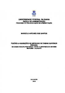
We consider the application of our convolution algorithm to two problems often encountered in practice. These are the computation of the Hilbert transform and the computation of the derivative. Both these functions are commonly determined either in the time domain by means of convolution with the appropriate operators or in the frequency domain. Results are of course identical if care is taken that the frequency domain computation represents discrete rather than circular convolution. Example l - n e Discrete Hilbert Transform: In general, the discrete Hilbert transform may be computed either by convolution with the Hilbert operator or by the 90" phase splitter method [9]. For comparison purposes, we have adopted the convolutional approach. Fig. l(a) shows the input signal which consists of two decaying sinusoids each represented as x ( t ) = exp ( - a j t ) sin ( 2 ? r t / T , + 8,) where cyl = 0.004, TI = 40 ms, O1 = 40", and a2 = 0.003, T2 = 75 ms, and 82 = 20". Fig. l(b) and (c) shows, respectively, the envelopes of the input signal determined by means of the normal approach and by means of the algorithm developed in this paper. Fig. l(d) and (e) shows the errors between the theoretical envelope and the envelopes shown in (b) and (c). Example 2-The Derivative: The second example which we consider is that of the computation of the derivative of a signal. The input signal which we consider is the same as shown in Fig. l(a). Fig. 2(a) and (b) illustrates the derivative computed using the standard convolutional approach and the recursive least squares approach, respectively. Fig. 2(c) and (d) shows the respective errors.
ZOO
lime (rnsec)
~.
~~
40
80
120
.
7
~~
I60
200
time (msec)
Fig. 1 . (a) Input signal consists of two decaying sinusoids each represented as x ( t ) = exp ( - a , r ) sin ( 2 ~ r / T + , 0,) where a , = 0.004. T , = 40 ms, 6, = 40". cx2 = 0.003. T, = 75 ms. and O2 = 20". (b) Envelope of the signal in (a) obtained using the normal frequency domain approach. (c) Envelope of the signal in (b) obtained using the algorithm developed in this paper. (d) Error between the true envelope and that shown in (b). (e) Error between the true envelope and that shown in (c).
L
11
I
time(msec)
Fig. 2. (a) Derivative of the trace shown in Fig. I(a) computed using the standard method in the frequency domain. (b) Derivative of the trace shown in (a) computed using the algorithm developed in this paper. (c) Error between the true derivative and that showsn in (a). (d) Error between the true derivative and that shown in (b).
convolution term, &, plays a fundamental role in the process, and the fidelity of the final result depends on f k in the same manner as Burg's autocovariance estimate depends on the initial zero lag value. We illustrate various examples of the use of our algorithm and, in particular, we show the marked improvement in the obtained convolution for the case of various filtering operations involving decaying harmonics. An interesting aspect of the method which we have presented relates to the convolution of signals which may be modeled as AR processes with zero innovation. In this case, for a particular order
1685
PORSANI A N D ULRYCH: DISCRETE CONVOLUTION
j , the forward and backward prediction errors, Ea,, and respectively, will be zero and the 2 j + 1 terms previously calculated may be extended indefinitely to the right and to the left of the computed series. The expressions for this particular case are immediately obtained from (22) and (23). These equations show that the forward and backward prediction operators, -a, and -b,, respectively, which allow the exact prediction of the signal for positive and negative times, also allow the exact prediction of the convolution to the left and to the right of the previous 2 j 1 convolution terms. This result demonstrates that the convolution of AR signals depends only on the forward and backward prediction operators and those convolution terms which are used to initialize the process. Another interesting aspect to the approach presented here occurs when we let the desired signal equal the input time series. In this case, the output of the algorithm is the autocorrelation of the input and, as before, the filters -U, and -bJ may be used to extend the autocorrelation function into positive and negative times to obtain the estimates r=,, and rLr. for order j . In order to ensure the nonnegative definite character of the autocorrelation function, these estimates may be averaged in a suitable manner as suggested in [ lo].
Substituting (A. 1) and (A.2) and simplifying, we obtain
APPENDIX We will assume knowledge of the modeling error operator of orderj, ( 1 h f ) , and the modeling error energy, E,,,j, which are related in the usual manner shown below:
The union of (A.6) and (A.7) allows the compact representation which we have used in the text
(A.4) where A,,, is determined from either of the expressions in (‘4.5)
+
-,
where the terms in the equation have been defined previously. We also assume knowledge of the P E 0 and of the prediction error energy of orderj which are related according to
eh,;
Let + I represent the quadratic form associated with the normal equations of orderj 1 for forward modeling
+
Substituting ( 1 hT+ ,) given by the Levinson recursion, we obtain for (A.3) [ l l ]
‘h,J
‘rd,,
+
rFr.jJ~hj,
(A.5a)
= rrd.j
+
r:d,jJJgjt
(A.5b)
=
with
rn,, = Minimizing
eh,,
( r L r , I ? rrr.27
>
* * *
rJ.
+ I with respect to h, + I , J + I results in ( A 4 h,+l,J+I
Substituting (A.6) into (A.4) results in the minimum error which is given by LEg,,
[
hJ+l,J+l
1
Eh,j+l.
(A.7)
A derivation of (10) in the text for backward modeling proceeds in an analogous manner. We emphasize that the procedure for obtaining the compact form (A.8) is not dependent on the Toeplitz character of the autocovariance matrix. Thus, the solution of the normal equations of o r d e r j 1 which contain a symmetric matrix may be obtained by means of the linear combination of solutions which satisfy forward and backward systems of orderj. We explore this fact in a forthcoming paper [ 121.
+
REFERENCES [ l ] J. P. Burg, “Maximum entropy spectrum analysis,” Ph.D. dissertation, Dep. Geophys., Stanford Univ., Stanford, CA, May 1975. [2] M. M o d , B. Dickinson, T. Kailath, and A. Vieira, “Efficient solution of covariance equations for linear prediction,” IEEE Trans. Acousr., Speech, Signal Processing, vol. ASSP-25, pp. 429-433, Oct. 1977. [3] E. T . Jaynes, “On the rationale of maximum-entropy methods.” Proc. IEEE, vol. 70, pp. 934-952, Sept. 1982. [4] N. Levinson, “The Wiener RMS (root mean square) error criterion in filter design and prediction,” J . Marh. Phys., vol. 25, pp. 261278, 1947. [5] T. J. Ulrych and R. W. Clayton, “Time series modelling and maximum entropy,” Phys. Earrh Planerar?, Inferiors, vol. 12, pp. 188200, Aug. 1976. [6] T. J. Ulrych, D. E. Smylie, 0. G. Jensen, and G. K. C. Clarke, “Predictive filtering and smoothing of short records by using maximum entropy,” J . Geophys. Res., vol. 78, pp. 4959-4961, Aug. 1982.
1686
IEEE TRANSACTIONS ON ACOUSTICS, SPEECH, AND SIGNAL PROCESSING, VOL. 37. NO. I I . NOVEMBER 1989
[7] S M Kay, “Maximum entropy estimation using the analytic signal,” IEEE Trans Acoust , Speech, SIgnal Processing, vol ASSP26, pp 467-469, Oct 1978 [8] S. Levy and D. W Oldenburg, “The deconvolution of phaseshifted wavelets,” Geophysics. vol. 47, pp 1285-1294, Aug 1987 [9] B Gold, A V Oppenheim, and C M Rader, “Theory and implementation of the discrete Hilbert transform,” in Proc Symp. Comput. Processing Commun., Brooklyn, NY, Apr 1969, pp. 235-250 [IO] P A Tyraskis and 0 G Jensen, “Multichannel autoregressive data models,” IEEE Trans. Geosci. Remote Sensing, vol. GE-21, pp 454463, 1983. [ l l ] M J Porsani and W J . Vetter, “An optimal formulation for (Levinson) recursive design of L-lagged minimum energy filters,” in Proc 54th Ann Int. Exploration Geophysicists (SEC) Meet , Atlanta, CA, Dec 1984, pp. 604-606 [12] M J Porsani and T J Ulrych, “Levinson-type extensions for nonToeplitz systems,” submitted to IEEE Trans Acoust , Speech, Signal Processing, 1989
research interests include time-series analysis and inverse theory i n geophysical exploration Dr Porsani I \ a member ot the Sociedade Brasileira de Geofisica (SBGF)
Tad J. Ulrych received the B.Sc degree (honors) Milton Porsani received the B Sc degree in geology from the University of Sao Paolo in 1976, the M.Sc. degree in geophysics from the University Federal do Para, and the Ph D degree in geophysics from the University Federal da Bahia in 1986. From 1978 to 1982 he was with NCGG-NuCleo de Ciencias Geofisicas e Geologicas, University Federal do Para. Since 1983 he has been a Researcher with the Programa de Pesquisa e PosGraduacao en Geofisica PPPGIUFBA, Brazil Hi5
from the University of London in 1957, and the M.Sc and Ph.D degrees from the University of British Columbia i n 1961 and 1963, respectively From 1962 to 1965 he was with the University of Western Ontario. Since 1965 he has been with the University of British Columbia. Since 1987 he has been a Visiting Professor at the Programa de Pesquisa e Pos-Graduacao en Geofisica PPPGI UFBA, Brazil His research interests include applications ot time-reries analysis and inverse theory to geophysical exploration Dr Ulrych received the Killan Fellowship i n 1983