Discrete Quantum Walks and Quantum Image Processing - CiteSeerX

Discrete Quantum Walks and Quantum Image Processing

Salvador El´ıas Venegas-Andraca Keble College University of Oxford Michaelmas Term, 2005

Thesis submitted for the degree of Doctor of Philosophy at the University of Oxford

Centre for Quantum Computation Atomic and Laser Physics Parks Road Oxford, OX1 3PU

Discrete Quantum Walks and Quantum Image Processing Abstract Salvador Elias Venegas-Andraca Keble College

Doctor of Philosophy Michaelmas Term 2005

In this thesis we have focused on two topics: Discrete Quantum Walks and Quantum Image Processing. Our work is a contribution within the field of quantum computation from the perspective of a computer scientist. With the purpose of finding new techniques to develop quantum algorithms, there has been an increasing interest in studying Quantum Walks, the quantum counterparts of classical random walks. Our work in quantum walks begins with a critical and comprehensive assessment of those elements of classical random walks and discrete quantum walks on undirected graphs relevant to algorithm development. We propose a model of discrete quantum walks on an infinite line using pairs of quantum coins under different degrees of entanglement, as well as quantum walkers in different initial state configurations, including superpositions of corresponding basis states. We have found that the probability distributions of such quantum walks have particular forms which are different from the probability distributions of classical random walks. Also, our numerical results show that the symmetry properties of quantum walks with entangled coins have a non-trivial relationship with corresponding initial states and evolution operators. In addition, we have studied the properties of the entanglement generated between walkers, in a family of discrete Hadamard quantum walks on an infinite line with one coin and two walkers. We have found that there is indeed a relation between the amount of entanglement available in each step of the quantum walk and the symmetry of the initial coin state. However, as we show with our numerical simulations, such a relation is not straightforward and, in fact, it can be counterintuitive. Quantum Image Processing is a blend of two fields: quantum computation and image processing. Our aim has been to promote cross-fertilisation and to explore how ideas from quantum computation could be used to develop image processing algorithms. Firstly, we propose methods for storing and retrieving images using non-entangled and entangled qubits. Secondly, we study a case in which 4 different values are randomly stored in a single qubit, and show that quantum mechanical properties can, in certain cases, allow better reproduction of original stored values compared with classical methods. Finally, we briefly note that entanglement may be used as a computational resource to perform hardware-based pattern recognition of geometrical shapes that would otherwise require classical hardware and software.

Acknowledgements “Together we stand, divided we fall”-Pink Floyd. I have spent several years of my life at the University of Oxford, a place full of wisdom, knowledge and mysticism. I have devoted my time to work towards a DPhil and to learn about the mysterious nature of human beings, about my own nature. In this journey I have sensed, as never before, the angel and the demon who simultaneously live in the human soul, in my soul. I want to devote the following lines to gratefully thank those who have believed in me, have inspired me to become a scientist and have helped my angel to defeat my demon. I want to thank my supervisors Dr. Sougato Bose and Professor Keith Burnett. Your support, knowledge, patience and guidance have been a key part of my doctoral degree. I have benefited not only from your scientific expertise and wisdom, but also from your warm bonhomie. Thank you very much for trusting me when I decided to do a DPhil at the Centre for Quantum Computation. I would not have come to Oxford University without the love, help and support of my family: My mother Amparo, my sister Samy, my step-father Bernardo, my aunt Noem´ı and my grand parents Margarita and Humberto. My dearest family, there are no words to say how much I love you. We have always been together, both in happiness and sadness, and I am immensely grateful for the gift of your love and company in my time on this Earth. I will always stand by you. I met a lovely woman in the last months of my time in Oxford. Her name is Annie Blaha and she gave me very strong reasons to believe that love really changes everything. Annie, with you I have finally understood the meaning of ‘love is a meeting of minds and a beating of hearts’. The people of México gave me a scholarship to read for a DPhil via our National Council for Science and Technology (scholarship No. 148528). México is more than my country: it is indeed my greatest passion. My gratitude and love to the people of México forever. I am also grateful for the financial assistance received from the Keble Association (Keble Open Scholarship), Oxford University Vice-chancellors’ Fund Award, Oxford University Physics Department (bursary), Centre for Quantum Computation (funding for Summer School on Quantum Information, Lisbon 2002), Keble College (hardship funds and funding to visit Caltech), and Institute for Quantum Information at Caltech (travel and maintenance expenses). The Centre for Quantum Computation has been a great place to do research and to socialise. I want to thank Dr. Jonathan Ball, Dr. Nikola Paunković, Dr. Luke Rallan, Dr. Alexander Hutton, Dr. Yasser Omar, Dr. Dan Browne and Dr. Garry Bowen for their friendship, enthusiasm and help. I have had the privilege of visiting several research centres where I have discussed and learned about several topics of my research fields. I thank Professor John Preskill from Caltech, Professor Artur Ekert from the University of Cambridge and Professor Vlatko Vedral from Imperial College and the University of Leeds for welcoming me to their research centres. Keble College has been a truly outstanding place to me. During my time in Oxford I had the pleasure to serve my college as MCR president and Junior Dean, and among those members of Keble College who certainly honor John Keble’s memory, I would like to thank: Penny Bateman, Roger Boden, David Bradley, Mark Butchers, Professor Averil Cameron, Alistair Cornell, Ken Downie, Dr. Sonia Mazey, Dr. Maria Misra, Dr. Anthony Phelan, Deborah Rogers, Dr. Alisdair Rogers, Ken Shaw, Isla Smith, Bill Thompson, Derek Waldron (my British step-dad) and Fred White. Friendship is a holy word. During my years at Oxford I met people whose capacity to think and to love goes far beyond any expectation. For their friendship, support and wisdom I would like to thank Dr. Natalia Arias Trejo (my dear friend comandanta Natalia, thank you very much for all you did for me and for México during our time in Oxford. You are one of the brightest women I have ever met in my life), Dr. Jonathan Ball (my British brother. Jon, thank you very much for showing me the best of Britain and for being a true citizen of the world), Bernard Cadogan (your friendship and our long talks on History, Philosophy, Poetry and life together with cigarettes and many bottles of wine, have left a deep mark in my heart. Thanks for sharing with me your world and wisdom), Dr. Barbara Casadei (the lovely physician who took care of my health during my time in Oxford. Barbara, thank you very much for saving my life), Mar´ıa Fernanda

González (supreme head of the Ex-A-Tec UK team, as well as my friend and confident), Jon Hafferty (my Junior Dean mate. Thanks for your support as colleague and friend), Mila Katzarova (for your friendship, your never-ending smile and those great dinners), Laura Malvaez (my dear Frida Kahlo, thanks for your friendship and high quality cuisine), Dr. Walterio Wolfang Mayol Cuevas (friendship, mathematics, politics and uncertainty, those are our topics), Dr. Paul Parrish (Paul, thank you very much for your friendship and for being a Patriot. People like you are the best the USA has to offer to Mankind), Dr. Nikola Paunković (my dear Serbian friend whom with I shared most of my thoughts and feelings during my time in Oxford), Dolores S´ anchez (our friendship and membership to Viajes Azteca will always remain with me), Felipe Villalobos (Chile, wine, Neruda and our common heritage are present whenever you and I engage in a conversation), and Justin Walker (thank you very much for being a good-natured man, for your friendship and kindness). I was honoured to serve my fellow countrymen and countrywomen as president of two organisations: the Oxford University Mexican Society and the Mexican Student Society in the United Kingdom. Among the people I had the honour and the privilege to meet, and whose support has been crucial during my time in Oxford, I would like to mention: Dr. Carlos Fuentes, whose intellectual leadership, tremendous support, warm friendship and generous words will be kept in my heart for the rest of my life. H.E. Juan José Bremer de Martino, Ambassador of México to the United Kingdom, for being an exemplary representative of my country, as well as for his continuous encouragement, support and wise advice. Professor David Brading, for those superb parties in his house, full of intelligent conversation and friendship. Ing. Cuauhtémoc Cárdenas, for his generosity, openess and willingness to share his thoughts and reflections. Minister Ignacio Dur´ an, for his zest for culture and his wise advice. Professor Alan Knight, for being generous with his time, support and advice, as well as for his always fascinating topics of conversation. Dr. Octavio Paredes, for his tremendous support and for being an outstanding leader as president of the Mexican Academy of Sciences. Dr. Juan Villoro, for his friendship and generosity, for welcoming me in Barcelona, and for our fantastic conversations ´ about México, literature and life. From CONACyT, I want to thank Silvia Alvarez-Bruneliere, for being sensible to the needs of CONACyT scholars abroad as well as for her very professional and fair problemsolving approach, and Roc´ıo Navarrete for her administrative support and readiness to help. Finally, big thanks to my dear friends Rodrigo Aguilar, Dr. José Bernardo Rosas, Dr. Erick Rosales and Dr. Axel Dom´ınguez for their teamwork and leadership during the foundation of MexSocUK. I was also honoured to be a founding member and vicepresident of Ex-A-Tec UK, the Alumni society of ITESM in the UK. I thank Mar´ıa Fernanda González, Osvel Garza, Jorge Pérez and Marco Muci˜ no for their friendship and for bearing with me and my rough problem-solving approach. I co-organised a Summer School on Quantum Computation in Mérida, Yucat´ an, in the summer of 2004. Among the people who worked very hard to make this summer school happen, I would like to thank Dr. Konrad Banaszek, Dr. Sougato Bose and Professor Vlatko Vedral (lecturers), Dr. Jonathan Ball, Dr. Yasser Omar and Dr. Nikola Paunković (workshop instructors), as well as Dr. Luis Alberto Mu˜ noz Ubando, Dr. Arturo Espinosa Romero and Dr. Romeo de Coss (co-organisers). I was given an award at the British Council International Student Awards 2005. Among those people who worked extremely hard to organise this magnificent event, I thank Melanie Stockwell and her team (British Council) and James Tibbert (International Office, University of Oxford). I also thank Luc´ıa Pérez Moreno (British Council, México), José Gal´ an (La Jornada), Claudia Arellano (Gaceta Ex-A-Tec) and Elizabeth Mistry (Mexican Wave and the Times Higher Educacion Supplement) for boosting my career (and therefore my potential contribution to México in the following years) with a series of articles about both my award and doctoral research. Many people from México have helped me and my family in several ways (even before I was born), and I want to let them know that I am truly grateful: Dr. Alejandro Aceves Gaona (our conversations when I was an undergraduate student as well as your friendship and honesty are immensely valuable to me), Ricardo Bola˜ nos (Ricardo, you have been a great friend to me. Both in hapiness and sadness, our friendship has been tested and I thank you for standing by me), Ra´ ul Comba (my dear Flaco, you have always been the silent voice that reminds me of my promises and facts. Thank you very much for that and for your friendship), Dr. Enrique Cortés Anguiano (my dear friend, I thank you for having shared the pleasures and sorrows of this life for so many years, as well as for showing me the beauty of your work and views on psychoanalysis), Rom´ an Cortés Anguiano (thank you very much for your friendship and for continuously challenging me to walk long distances, to defeat my weaknessess), Dr. Arturo Espinosa Romero (many years of being friends and sharing

cigarettes together with dreams and experiences about science and scouting), Dr. Jes´ us Figueroa Nazuno (for your support and advice when I was planning on coming to Oxford), Jorge Arturo Filio Rivera (Jorge, we have been friends for most of our lives and, after all we have been through, I can only say that I am immensely happy to know that we count on each other), Martha Ofelia Hernández Guzm´ an (T´ıa Martha, thank you for your love and for being always close to my mother), Roberto Inguanzo(†) (my dear godfather, I thank you for being a true friend to my mother), Francisco Crist´ obal III Lanz Rodr´ıguez (my dear friend, I can only say that you are one of the greatest blessings I have ever been given in my life) and his wife Guadalupe Villalvaso (comadre and friend, thank you very much for your words and support), Dr. Luis Alberto Mu˜ noz Ubando (my dearest friend, thank you very much for your continuous support and our joint ventures. Your example and enthusiasm took me to Oxford), Ydalio Pérez Centeno (Q ∴ H ∴ Ydalio, thank you very much for sharing your wisdom with me and for your continuous support), Connie Rodr´ıguez (friendship and faith are the pillars of our communication), Dr. Juan Manuel Rodr´ıguez Penagos (Mane, thank you very much for your friendship and for those great parties and psychoanalysis lectures), Lilia Rosal Balduc (Lilia, your support to me and to my family has been crucial. Thanks to your friendship and help, I did my first degree and have had time to expand on my scientific and intellectual interests. I will never forget what you have done for me and for my family), David S´ anchez and his wife Angelita Venegas (David, Angelita, thank you very much for standing by us when we most needed it), José Santiago Reuss and his family (Pepe, thank you very much for your kind friendship and for being with us when we had to swallow bitter pills), Dr. Rafael Sarti (Rach, I thank you not only for your friendship but also for being such a great physician to me), Dr. Horacio Trillo (for your friendship and those unforgettable meetings on science and culture), Mario Vargas (my dear Mario, we have been given what we were promised: friendship and an unbreakable hope of a better future, that is, faith), Gema Venegas and her husband Marco Antonio Acosta (thank you very much Gema and Marco, for being with us when we most needed it), and Enrique Zamora Gallardo (for your friendship, support and those great conversations on science and culture). Before finishing my acknowledgements, I want to thank the women of my life. Although I will not say their names here, I want them to know that I have spent with them some of the best moments of my life. Thank you very much for those bits of your lives and hearts you shared with me. This is my way to definitely say good bye and to wish you well. And, last but never least, I thank Jesus of Nazareth, the man who became my friend and my God because of his brave heart and endless love.

Dedication

This work is dedicated to My family: Amparo, Samy, Bernardo, Noem´ı, Ricardo(†) , Margarita(†) and Humberto(†) . The memories of President Benito Pablo Ju´ arez Garc´ıa and General Emiliano Zapata. The Mexican patriots who paid for my freedom with their lives: Independence and Revolution wars, and 1968 student revolt. My beloved M´ exico.

List of publications 1. [180] Quantum Computation and Image Processing: New Trends in Artificial Intelligence by S.E. Venegas-Andraca and S. Bose. Proceedings of the International Conference on Artificial Intelligence IJCAI-03 (peer-reviewed). 2. [181] Storing, processing and retrieving an image using Quantum Mechanics by S.E. Venegas-Andraca and S. Bose. Proceedings of the 2003 SPIE Conference on Quantum Information and Quantum Computation. 3. [178] Storing Images in Entangled Systems by S.E. Venegas-Andraca and J.L. Ball. Submitted to IEEE Transactions on Image Processing. 4. [179] Quantum Walks with Entangled Coins S.E. Venegas-Andraca, J.L. Ball, K. Burnett and S. Bose New Journal of Physics 7 221 (2005). 5. Quantum Walks with Entangled Coins and Walkers in Superposition by S.E. VenegasAndraca, J.L. Ball, K. Burnett and S. Bose (in preparation). 6. Entanglement Generation in Quantum Walks by S.E. Venegas-Andraca, K. Burnett and S. Bose (in preparation).

Contents 1 Introduction

1

2 Quantum Mechanics 2.1 Mathematical preliminaries . . . . . . . . . . 2.2 Postulates of Quantum Mechanics . . . . . . 2.2.1 State space . . . . . . . . . . . . . . . 2.2.2 Evolution of a closed quantum system 2.2.3 Quantum measurements . . . . . . . . 2.2.4 Composite quantum systems . . . . . 2.3 Entanglement . . . . . . . . . . . . . . . . . . 2.3.1 Measure of entanglement . . . . . . . 2.3.2 Bell inequalities . . . . . . . . . . . . .

. . . . . . . . .

. . . . . . . . .

. . . . . . . . .

. . . . . . . . .

. . . . . . . . .

. . . . . . . . .

. . . . . . . . .

. . . . . . . . .

. . . . . . . . .

. . . . . . . . .

. . . . . . . . .

. . . . . . . . .

. . . . . . . . .

. . . . . . . . .

. . . . . . . . .

. . . . . . . . .

. . . . . . . . .

. . . . . . . . .

. . . . . . . . .

. . . . . . . . .

. . . . . . . . .

. . . . . . . . .

11 12 17 17 20 21 22 23 24 25

3 Theory of Computation 3.1 What is the Theory of Computation? . . . . . . . . . 3.2 Hilbert’s program and the Entscheidungsproblem . . 3.3 On Computability . . . . . . . . . . . . . . . . . . . 3.4 Definition of a Problem and two examples . . . . . . 3.5 Models of Computation and Algorithmic Complexity 3.5.1 Asymptotic Notation . . . . . . . . . . . . . . 3.5.2 Deterministic Finite Automata . . . . . . . . 3.5.3 Nondeterministic Finite Automata . . . . . . 3.5.4 Deterministic Turing Machines . . . . . . . . 3.5.5 Algorithmic Complexity for DTMs . . . . . . 3.5.6 Nondeterministic Turing Machines . . . . . . 3.5.7 Algorithmic Complexity for NTMs . . . . . . ? 3.5.8 P = NP and NP-complete problems . . . . 3.6 Physics and the Theory of Computation . . . . . . .

. . . . . . . . . . . . . .

. . . . . . . . . . . . . .

. . . . . . . . . . . . . .

. . . . . . . . . . . . . .

. . . . . . . . . . . . . .

. . . . . . . . . . . . . .

. . . . . . . . . . . . . .

. . . . . . . . . . . . . .

. . . . . . . . . . . . . .

. . . . . . . . . . . . . .

. . . . . . . . . . . . . .

. . . . . . . . . . . . . .

. . . . . . . . . . . . . .

. . . . . . . . . . . . . .

. . . . . . . . . . . . . .

. . . . . . . . . . . . . .

. . . . . . . . . . . . . .

. . . . . . . . . . . . . .

27 27 28 29 30 32 33 34 36 38 40 42 43 44 46

4 Classical Discrete Random Walks 4.1 Probability theory and stochastic processes . . . . . 4.1.1 Discrete Random variables and distributions 4.1.2 Moments and generating functions . . . . . . 4.1.3 Markov chains . . . . . . . . . . . . . . . . . 4.2 Classical random walks: results and applications . . 4.2.1 Classical Random Walks on a Line . . . . . .

. . . . . .

. . . . . .

. . . . . .

. . . . . .

. . . . . .

. . . . . .

. . . . . .

. . . . . .

. . . . . .

. . . . . .

. . . . . .

. . . . . .

. . . . . .

. . . . . .

. . . . . .

. . . . . .

. . . . . .

. . . . . .

49 49 49 51 54 57 58

i

. . . .

. . . .

. . . .

. . . .

. . . .

. . . .

. . . .

. . . .

. . . .

. . . .

. . . .

. . . .

. . . .

. . . .

. . . .

. . . .

. . . .

. . . .

. . . .

61 68 68 71

5 Discrete Quantum Walks 5.1 Quantum walk on a line . . . . . . . . . . . . . . . . 5.1.1 Structure of a DQWL . . . . . . . . . . . . . 5.1.2 Analysis of quantum walks on an infinite line 5.1.3 Quantum walk with boundaries . . . . . . . . 5.2 Quantum walks on graphs . . . . . . . . . . . . . . . 5.3 Algorithmic applications of quantum walks . . . . .

. . . . . .

. . . . . .

. . . . . .

. . . . . .

. . . . . .

. . . . . .

. . . . . .

. . . . . .

. . . . . .

. . . . . .

. . . . . .

. . . . . .

. . . . . .

. . . . . .

. . . . . .

. . . . . .

. . . . . .

. . . . . .

73 75 76 78 92 93 99

4.3

4.2.2 Classical random walks on Randomized algorithms and SAT 4.3.1 2-SAT . . . . . . . . . . . 4.3.2 3-SAT . . . . . . . . . . .

a graph . . . . . . . . . . . . . . .

. . . .

. . . .

. . . .

. . . .

. . . .

6 Quantum Walks and Entanglement I 6.1 Introduction . . . . . . . . . . . . . . . . . . . . . . . . . . . . . . . . . . . . . . . . . 6.2 Classical Random Walk with 2 Maximally Correlated Coins . . . . . . . . . . . . . . 6.3 Quantum Walks with Entangled Coins . . . . . . . . . . . . . . . . . . . . . . . . . . 6.3.1 Mathematical Structure of Quantum Walks on an Infinite Line Using a Maximally Entangled Coin . . . . . . . . . . . . . . . . . . . . . . . . . . . . . . . 6.3.2 Results for Quantum Walks on an Infinite Line Using a Maximally Entangled Coin . . . . . . . . . . . . . . . . . . . . . . . . . . . . . . . . . . . . . . . . . 6.4 Quantum Walks using coins with different entanglement values . . . . . . . . . . . . 6.5 Quantum walks with more than two maximally entangled coins . . . . . . . . . . . . 6.6 Conclusions and Outlook . . . . . . . . . . . . . . . . . . . . . . . . . . . . . . . . .

104 104 109 110

7 Quantum Walks and Entanglement II 7.1 Quantum Walks with Entangled Coins and Walkers in Superposition . . . 7.1.1 Quantum walks with one walker in uniform superposition . . . . . . 7.1.2 Quantum walks with one walker in Gaussian superposition . . . . . 7.2 Entanglement Generation in Quantum Walks . . . . . . . . . . . . . . . . . 7.2.1 Entanglement Generation in unrestricted Quantum Walks on a Line 7.3 Conclusions and Outlook . . . . . . . . . . . . . . . . . . . . . . . . . . . .

. . . . . .

. . . . . .

. . . . . .

. . . . . .

. . . . . .

126 127 129 133 134 135 142

8 Quantum Image Processing 8.1 Storing an image using quantum mechanics . . . . . . . . . . . . 8.1.1 Previous Work . . . . . . . . . . . . . . . . . . . . . . . . 8.1.2 Storing an Image in a Quantum System . . . . . . . . . . 8.1.3 Storing Colour in a qubit . . . . . . . . . . . . . . . . . . 8.1.4 Storing an Image in a Qubit Lattice . . . . . . . . . . . . 8.1.5 Retrieving an Image from a Quantum System . . . . . . . 8.1.6 Retrieving a single frequency . . . . . . . . . . . . . . . . 8.1.7 Retrieving a full Image . . . . . . . . . . . . . . . . . . . . 8.1.8 Quantum vs classical storage and retrieval of information 8.2 Storing Images in Entangled Quantum Systems . . . . . . . . . . 8.2.1 Quantum Entanglement . . . . . . . . . . . . . . . . . . . 8.2.2 New method for storing images . . . . . . . . . . . . . . . 8.2.3 Use of entanglement for scale-invariant shape recognition

. . . . . . . . . . . . .

. . . . . . . . . . . . .

. . . . . . . . . . . . .

. . . . . . . . . . . . .

. . . . . . . . . . . . .

149 151 151 152 152 153 155 155 156 157 160 160 162 166

ii

. . . . . . . . . . . . .

. . . . . . . . . . . . .

. . . . . . . . . . . . .

. . . . . . . . . . . . .

. . . . . . . . . . . . .

. . . . . . . . . . . . .

110 114 119 122 124

8.3

Summary and Outlook . . . . . . . . . . . . . . . . . . . . . . . . . . . . . . . . . . . 166

9 Conclusions 168 Appendix I . . . . . . . . . . . . . . . . . . . . . . . . . . . . . . . . . . . . . . . . . . . . i Appendix II . . . . . . . . . . . . . . . . . . . . . . . . . . . . . . . . . . . . . . . . . . . . iii References . . . . . . . . . . . . . . . . . . . . . . . . . . . . . . . . . . . . . . . . . . . . . 1

iii

Chapter 1

Introduction Quantum Mechanics and the Theory of Computation are two of the most important intellectual achievements of the 20th century. These two branches of science have not only inspired several generations of scientists and thinkers, they have also had a significant impact in the daily life of Mankind, from war to literature (two recent examples of works in literature inspired by the ideas and history of quantum mechanics are [33] and [185]). As a matter of fact, cross-fertilisation between physics and computation has been abundant due to the fact that many ideas, concepts and technological developments from both fields have been used to advance knowledge in each discipline. One of the most recent joint ventures between physics and the theory of computation is Quantum Computation. Quantum computation can be defined as the scientific field whose purpose is to solve problems with finite time procedures, i.e. algorithms, which exploit the quantum mechanical properties of those physical systems used to implement such algorithms. The academic background of the author of this thesis includes several branches of theoretical and applied computer science. Consequently, our approach in the development of this thesis has been to study those concepts of quantum mechanics and quantum computation relevant to the computational aspects of the fields we have focused on: Discrete Quantum Walks and Quantum Image Processing. Thus, in the history of cross-fertilisation between physics and computation, this thesis is meant to be situated as a contribution within the field of quantum computation from the perspective of a computer scientist. Let us now briefly review our contributions in the fields we have worked on. 1

2 Discrete Quantum Walks. In order to provide a definition of the field of discrete quantum walks, we first introduce the concept of a stochastic algorithm. In the following paragraphs we shall assume that, in principle, the problems we intend to solve by using an algorithmic approach are indeed solvable by such a method. There are several ways to design solutions (i.e. to develop algorithms) in computer science. For example, a powerful method consists of defining a set of rules such that for a given step i in algorithm A, we can always fully determine step i+ 1, i.e. at any point of the execution of algorithm A we can be fully certain about the next step to be performed, as long as we know the rules of logic used to develop A. Algorithms developed under this methodology are known as deterministic algorithms because it is always possible to determine the exact behaviour of those algorithms, just by knowing the starting conditions and the set of rules used for algorithm development. Another method used in algorithm design makes use of chance. In this approach, for a given step i of algorithm A, step i + 1 cannot be fully determined as there are several possible next steps. The actual step i + 1 that will be carried out is chosen from a set of possible next steps with the help of a probability distribution (usually, the uniform distribution). This family of algorithms is known as stochastic algorithms and plays a most important role in computer science due to the fact that, in some cases, the most efficient (or least inefficient, depending on the point of view) algorithms known so far for solving certain kinds of problems, are stochastic ([134] and [163]). Classical random walks, a subset of stochastic processes (that is, processes whose evolution involves chance), have proved to be a very powerful tool for the development of stochastic algorithms [134]. The main idea behind the mechanics of classical random walks is the following: assume we have a particle (walker) that is allowed to move on a lattice. The actual movements of the particle on the lattice, i.e. the evolution of the system, are performed according to a probability distribution. A simple example is the following: suppose that we have a particle on a line, and that the motion of that particle on a line (i.e. moving to the left or to the right) is performed according to the outcomes of tossing a coin (for example, heads → right and tails → left). This process is clearly stochastic and it is known as a classical random walk on a line. Given the importance of classical random walks in algorithm development, there has been an increasing interest in studying quantum counterparts of classical random walks, known as quantum

3 walks, in order to develop new quantum algorithms. As we shall see in corresponding chapters, there is already a series of quantum algorithms based on quantum walks that outperform their classical counterparts. However, the field of quantum walks is very young and more research is needed in order to understand how to make full use of this discipline in quantum computation. There are two main sets of quantum walks: discrete and continuous quantum walks. The main difference between these two sets is the timing used to apply corresponding evolution operators. In the case of discrete quantum walks, the corresponding evolution operator of the system is applied only in discrete time steps, while in the continuous quantum walk case, the evolution operator can be applied at any time. In this thesis we concentrate on discrete quantum walks, although we review a most important application of continuous quantum walks for algorithm development in chapter 5. Our contribution in the field of quantum walks can be summarised as follows. Firstly, we have proposed a model of discrete quantum walks on an infinite line with the following initial conditions: a) Pairs of quantum coins under different degrees of entanglement, and b) Quantum walkers in different initial state configurations, including superpositions of corresponding basis states. Among our results we have found several properties on the symmetry of probability distributions computed from those quantum walks, as well as numerical evidence that some of those symmetry properties are not straightforwardly related to the initial conditions of the quantum walk. This fact is important because, in the classical world, the long-run (asymptotical) behaviour of classical random walks on certain topologies does not generally depend on the initial conditions. Secondly, we have studied the properties of the entanglement generated between walkers, in a family of quantum walks on an infinite line with one coin and two walkers. The main idea here is the following. Start a quantum walk with a triple tensor product: one particle as coin and two particles as walkers, and quantify the amount of entanglement between walkers at each time step (of course, we perform many quantum walks with the same initial conditions and evolution operators, in order to have one quantum walk ready to be measured for each time step). As we show in the following chapters, there is indeed a relation between the amount of entanglement available in each time step and the symmetry of the initial coin state. However, as we also show with our numerical simulation results, this relation is not straightforward and, in fact, such a relation can be counterintuitive.

4

Our contributions in this field can be found in: 1. [179] Quantum Walks with Entangled Coins S.E. Venegas-Andraca, J.L. Ball, K. Burnett and S. Bose New Journal of Physics 7 221 (2005). 2. Quantum Walks with Entangled Coins and Walkers in Superposition by S.E. VenegasAndraca, J.L. Ball, K. Burnett and S. Bose (in preparation). 3. Entanglement Generation in Quantum Walks by S.E. Venegas-Andraca, K. Burnett and S. Bose (in preparation). Quantum Image Processing. Due to the fact that the academic background of the author includes the fields of Artificial Intelligence and Robotics, and that the potential use of quantum mechanical systems in disciplines like artificial intelligence and pattern recognition is an exciting and mostly unexplored research field with just a few introductory works published so far (for example, [87], [94], [173], [174] and [182]), part of our research efforts were devoted to create some links between quantum computation and Image Processing, an area of applied computer science and computer engineering widely used in artificial intelligence, pattern recognition and robotics. Broadly speaking, Image Processing can be defined as the branch of computer science and engineering that focuses on storing, manipulating and retrieving visual information in computer systems. The technical processes of storing, manipulating and retrieving visual information lay within the scope of computer architecture engineering, while the performance and constraints of algorithms used in this field are found within the scope of computer science. We have coined the term Quantum Image Processing to refer to this blend of ideas from quantum computation and image processing. We underline that our contributions do not fully fall within the realm of physics, that is, the ideas and methods developed in our work were not directed towards presenting new results within the field of quantum computation. Instead, our aim in this field has been twofold, being the first one to build a bridge, to construct a common language between the fields of quantum computation and image processing with the objective of promoting cross-fertilisation. Secondly, we wanted to explore how the concepts and techniques of quantum computation would actually help computer practitioners to develop better algorithms. Our contributions can be summarised as follows. Firstly, we propose a method for storage and retrieval of an image in a multi-particle quantum mechanical system. We consider a situation in which non-entangled qubits replace classical bits in an array of pixels and show several advantages.

5 Additionally, we study a case in which 4 different values are randomly stored in a single qubit, and show that quantum mechanical properties allow better reproduction of original stored values compared with classical methods. The retrieval process is uniquely quantum as it involves measurement in more than one basis. Secondly, we present a method for storing and retrieving images using maximally entangled qubits. We show that using entanglement as a computational resource allows us to do some hardware-based pattern recognition processes that would otherwise require the use of hardware and software in the classical world. Our contributions can be found in: 1. [178] Storing Images in Entangled Systems by S.E. Venegas-Andraca and J.L. Ball. Submitted to IEEE Transactions on Image Processing. 2. [180] Quantum Computation and Image Processing: New Trends in Artificial Intelligence by S.E. Venegas-Andraca and S. Bose. Proceedings of the International Conference on Artificial Intelligence IJCAI-03. The IJCAI is a most prestigious conference on artificial intelligence and, consequently, all papers and posters published in the proceedings are peer-reviewed. 3. [181] Storing, processing and retrieving an image using Quantum Mechanics by S.E. Venegas-Andraca and S. Bose. Proc. of the 2003 SPIE Conference on Quantum Inf. and Quantum Computation. It has been the intention of this author to write a thesis from which both physicists and (theoretical as well as applied) computer scientists can gain a solid knowledge about the fields of discrete quantum walks and quantum image processing. Additionally, the introductory chapters can also be used to understand some basic elements of quantum computation. In addition to our original contributions in both quantum walks and quantum image processing, physicists may use this thesis as a concise guide to understand the main elements of the theory of computation and the profound mathematical roots of this discipline. For computer scientists, our thesis may be used to obtain a succint guide to some of the concepts of quantum mechanics needed to be initiated in the fields of quantum walks and quantum computation. This thesis has been partly motivated by our wish to build a common language between different disciplines: quantum computation and several areas of applied computer science. In our opinion, having people from applied areas of computer science on board will give quantum computation an additional momentum as well as new and challenging problems to work on.

6 In addition to the scientific contents of this thesis, we have tried to provide a succint guide to the historical evolution of ideas in our fields, as well as to hint at links between thinkers and their contributions where possible. The rationale behind this feature is the fact that the author of this thesis truly believes that, in order to fully understand and appreciate the evolution and beauty of scientific concepts and theories, it is of great help to be aware of the historical roots of those ideas. After all, Science is a human invention and History is a fundamental part of our culture. We now provide an outline of our thesis. Chapter 2. Quantum Mechanics. This chapter is a concise introduction to the postulates of quantum mechanics (and the mathematical tools required to formulate those postulates) needed to understand the main concepts and techniques of quantum walks and quantum image processing, as well as some of the foundational elements of quantum computation. We also provide a succint introduction to entanglement because we shall use this quantum mechanical property in our contributions chapters (6, 7 and 8). Additionally, we briefly review Bell inequalities because we shall use them in chapter 8 in the context of entanglement detection for quantum image processing. This chapter has been written with two purposes in mind: 1) to provide the necessary background for our work on quantum walks and quantum image processing, and 2) to serve as a concise guide for computer scientists who need to grasp those elements of quantum mechanics required to be initiated in the fields of quantum computation, quantum walks and quantum image processing. In this sense, this chapter is meant to be taken as a resource for studying such fields. Chapter 3. Theory of Computation. We begin by briefly revisiting the historical roots of the mathematical development of Turing machines, followed by the enunciation of the Church-Turing thesis and the definition of decision problems in the context of computer science. We then proceed to formally define deterministic and nondeterministic finite automata, two models of computation that are used later on to define both deterministic and nondeterministic Turing machines. We also introduce some formal elements of algorithmic complexity (mainly, measures used to quantify the performance of an arbitrary algorithm), followed by the topic of NP-completeness, one of the central themes in Complexity Theory, together with an example of NP-completeness: the satisfiability (SAT) problem. Finally, we provide a brief review on the links between physics and the theory of computation and we give the definitions of Probabilistic and Quantum Turing machines.

7 Chapter 4. Classical Discrete Random Walks. The goal of this chapter is to provide a short but rigorous introduction to those properties of classical discrete random walks on undirected graphs relevant to algorithm development. We start by offering some basic elements of probability theory (several probability distributions, Markov’s inequality and moments of probability distributions), followed by definitions and theorems of Markov chains and stationary probability distributions. We introduce the definition and main results of classical random walks on a line with three variants: no barriers, one absorbing barrier and two absorbing barriers. In order to get more general results, we introduce classical random walks on (Cayley) graphs and present two measures used to quantify the performance of classical random walks in algorithm development: hitting time and mixing time. The last part of this chapter begins with an analysis on the hitting and mixing times of a classical random walk on an unrestricted line. This analysis is, to the best of this author’s knowledge, an original contribution to the field of classical random walks, at least in the form that information is presented and the explicit method used to quantify the hitting time of a classical random walk on an unrestricted line. Basically, we show that the hitting time of a classical discrete random walk on an unrestricted line depends on the region we locate the walker in (we divide the line into two regions: the first one is the area within a distance roughly equal (up to a constant factor) to the standard deviation of the binomial distribution from the starting point of the walk, and the second is the rest of the line). Thus, if we use the hitting time of this random walk to quantify its corresponding mixing time (this is a usual practice in classical random walks), we find that the calculation of the mixing time of a classical random walk on an unrestricted line is not straightforward. This becomes an obstacle for comparing the performance of an unrestricted classical random walk on a line with its quantum counterpart. We will come back to this comparison shortly. After studying the unrestricted classical random walk on a line, we quantify the hitting and mixing times of classical random walks on a line with two reflecting barriers, and on a circle. We finish this chapter by providing a detailed analysis of the randomised algorithms used to solve two versions of the SAT problem: 2-SAT and 3-SAT.

8 Chapter 5. Discrete Quantum Walks. In this chapter we offer a comprehensive yet concise introduction to the main concepts, results and algorithmic applications of discrete quantum walks on a line and on a graph. We first outline the main motivations for doing research in this field, followed by the mathematical description of the components of a quantum walk on a line. We continue with a detailed analysis of the Hadamard quantum walk on an infinite line, using a method based on the Discrete Time Fourier Transform known as the Schr¨ odinger approach. This analysis includes the enunciation of relevant theorems, as well as the advantages of the Hadamard quantum walk on an infinite line with respect to its closest classical counterpart. In particular, we explore the context in which the properties of the Hadamard quantum walk on an infinite line are compared with classical random walks on an infinite line and with two reflecting barriers. Also, we briefly review another method for studying the Hadamard walk on an infinite line: path counting approach. We then proceed to study a quantum walk on an infinite line with an arbitrary coin operator. In particular, we explain what is meant by stating that the study of the Hadamard quantum walk on an infinite line is enough as for the analysis of arbitrary quantum walks on an infinite line. To finish with our review on quantum walks on a line, we present the main results of quantum walks on a line with one and two absorbing barriers. We then focus on the properties of quantum walks on graphs. We study quantum walks on a circle, on the hypercube and some general properties of quantum walks on Cayley graphs. Finally, we review the algorithmic applications of quantum walks. We start by analysing the most successful quantum algorithm based on a (continuous) quantum walk, which consists of traversing, in polynomial time, a family of graphs of trees with an exponential number of vertices (the same family of graphs would be traversed only in exponential time by any classical algorithm), and finish with a review on search algorithms based on quantum walks. Note on chapters 3,4 and 5. Because of the author’s background in computer science, he was encouraged by one of his supervisors, Professor K. Burnett, to make a thorough review of those computational issues that would help the reader to understand the significance of classical random walks and quantum walks in computer science. Therefore, the material contained in chapters 3, 4 and 5, although technically a review, contains a critical assessment of a number of important issues. The purpose of this critical assessment is twofold: 1) To provide a clear and solid explanation of

9 main concepts and theorems of classical and quantum walks relevant to algorithm development (for example, the mathematical tools and methods from classical random walks used to solve 2-SAT and 3-SAT), and 2) to clarify some concepts and methods used to compare and evaluate the performance of classical and quantum walks (for example, the topologies used to compare the performance of a quantum walk on an infinite line with its closest classical counterparts). Chapter 6. Quantum Walks and Entanglement I. In this chapter we present new material, based on our paper [179]. As stated at the beginning of this introduction, we introduce a mathematical formalism for the description of unrestricted quantum walks on a line with maximally entangled coins and one walker. The numerical behaviour of such walks is examined when using a Bell state as the initial coin state, two different coin operators, two different shift operators, and one walker. Additionally, we compare and contrast the performance of these quantum walks with that of a classical random walk consisting of one walker and two maximally correlated coins as well as quantum walks with coins sharing different degrees of entanglement. We illustrate that the behaviour of our walk with entangled coins can be very different in comparison to the usual quantum walk with a single coin. We also demonstrate that simply by changing the shift operator, we can generate widely different distributions. We also compare the behaviour of quantum walks with maximally entangled coins with that of quantum walks with nonentangled coins. Finally, we show that the use of different shift operators on 2 and 3 qubit coins leads to different position probability distributions in 1 and 2 dimensional graphs. Chapter 7. Quantum Walks and Entanglement II. This is our second chapter with original contributions. We begin by presenting our results on a generalisation of [179], which consists of a study on quantum walks on an infinite line with the following initial conditions: bipartite coin initial state |coini0 ∈ Hc4 with different degrees of entanglement, and walker initial state |walkeri0 ∈ Hp in uniform and Gaussian superposition of a subset of basis states |ii ∈ Hp . We also study the generation of entanglement in unrestricted quantum walks on a line with one coin and two walkers. After evolving the quantum walk for a certain number of steps, we perform a measurement on the coin state. We then obtain a post-measurement quantum state composed by the tensor product of one coin state and several walker components. We take the walker components of this post-measurement state and calculate the entanglement between walkers. We perform many

10 quantum walks with the same initial conditions and evolution operators, so that we have a quantum walk ready to be measured for each time step. An outline of the simulation method used to produce chapters 6 and 7 can be found in appendix II. Chapter 8. Quantum Image Processing. This is our third and last chapter on original contributions, based on [178], [180] and [181]. We propose a method to store and retieve images in a multi-particle quantum mechanical system. We replace classical bits with non-entangled qubits in an array of pixels and show several advantages. Also, we study a case in which 4 different values are randomly stored in a single qubit, and show that quantum mechanical properties allow better reproduction of original stored values compared with classical methods. Secondly, we introduce a procedure to store and retrieve images using maximally entangled qubits. We show that using entanglement as a computational resource allows us to do some hardware-based pattern recognition processes that would otherwise require the use of hardware and software in the classical world. Chapter 9. Conclusions. Here we present our conclusions on the ideas developed in this thesis, as well as our next research steps. We finish this introduction with a critical list of articles and books that would provide the reader with a good introduction to the fields we have discussed in this thesis. Introduction to quantum mechanics for quantum computation. [31], [85] and [137]. Theory of computation and complexity theory: [52], [142] and [167]. Classical discrete random walks. Basic concepts of classical random walks can be found in [48], [83] and [188]. For concepts of classical random walks relevant to algorithm development, the reader may find the following sources useful: [127], [128], [134] and [150]. Quantum Walks. [105] is a good introductory article. Main results on quantum walks on an infinite line can be found in [10], [136], [40] and [171], and results on quantum walks with boundaries are given in [13]. Main definitions and theorems on quantum walks on graphs are given in [4], [133] and [106]. Finally, algorithmic applications of quantum walks may be read from [43], [165] and [7]. Applications of quantum computation in pattern recognition and neural networks. [172], [173] and [87]. Finally, the following PhD theses were extremely useful: [32], [99], [34], [144], [149], [74] and [103].

Chapter 2

Quantum Mechanics Quantum mechanics is the description of the behaviour of matter and light in all its details and, in particular, of the behaviour of Nature on an atomic scale [68]. Indeed, quantum mechanics plays a fundamental role in the description and understanding of natural phenomena [47]. The history (1900 - circa 1930) behind the experimental and conceptual development of quantum mechanics is a fascinating recollection of scientific experiments and interpretation of experimental results, along with a constant challenge of ideas and assumptions held about Nature for long time ([58], [89] and [148]). Thanks to the works begun by W. Heisenberg and E. Schr¨ odinger, and followed by many other physicists like R. Feynman and M. Born, quantum mechanics has now a well developed mathematical structure that provides scientists with a precise theoretical framework with which they can predict the behaviour of physical systems. Although there is still debate and controversy about several elements and interpretations of quantum mechanics, using this theory to analyse and predict the behaviour of physical systems has proven very fruitful. The birth of Quantum Computation and Quantum Information is a consequence of combining ideas from Quantum Mechanics, Computer Science and Information Theory. We review those concepts of quantum mechanics needed to understand the main ideas contained in the fields of Quantum Computation and Quantum Walks. In this thesis we have explicitly avoided the topic of interpretations of quantum mechanics, as our interests are focused on the use of quantum mechanics in quantum computation and quantum walks, with the purpose of developing quantum algorithms. We have written this chapter having in mind not only physicists but also computer 11

12

2.1 Mathematical preliminaries

scientists interested in these fields. We start by providing some mathematical preliminaries followed by the postulates of quantum mechanics. We then present entanglement and finish this chapter with a discussion on Bell inequalities. This chapter is based on [17], [31], [47], [55], [68], [85] and [137]. Additionally, [153] is a concise introduction to quantum mechanics and quantum computation for non-physicists, and [45] a useful review of entanglement quantification.

2.1

Mathematical preliminaries

We begin with a central element for the formulation of quantum mechanics: Hilbert spaces. Definition 2.1.1. Inner-product vector space. An inner-product vector space V is a complex vector space, equipped with an inner-product h·|·i : V × V → C, satisfying the following axioms. ∀ a, b, c, d ∈ V, α, β ∈ C 1) ha|bi = hb|ai∗ 2) ha|ai ≥ 0 and ha|ai = 0 ⇔ a = 0 3) ha|αb + βci = αha|bi + βha|ci The inner product introduces the norm on V: ||a|| =

p

ha|ai

Definition 2.1.2. Complete inner-product vector space. An inner-product vector space V is called complete if for any sequence {ai }∞ i=1 , ai ∈ V with the property limi,j→∞ ||ai − aj || = 0, there is a unique element b ∈ V such that limj→∞ ||b − aj || = 0. Definition 2.1.3. Hilbert space. A Hilbert space H is a complete inner-product vector space1 . Two Hilbert spaces H1 and H2 are said to be isomorphic if the underlying vector spaces are isomorphic and their isomorphism preserves the inner product.

2

Definition 2.1.4. Functional. Let V be a vector space over a field F . A linear functional is a linear function f : V → F . 1 Complete inner-product spaces were baptised as Hilbert spaces by J. von Neumann, due to the studies made by D. Hilbert on linear integral systems. In the following chapter we shall see that D. Hilbert also played an important role in the birth and development of the Theory of Computation. 2 In linear algebra, an isomorphism can also be defined as a linear map between two vector spaces that is one-to-one and onto.

13


Lemma 1. [85] Inner-product as linear mapping. Let H be a Hilbert space. Then, for each a ∈ H the function fa : H → C defined by fa (b) = ha|bi is a linear mapping. Therefore, function fa is a functional. Theorem 1. [85]. To each continuous linear mapping f : H → C there exists a unique φf ∈ H such that f (ψ) = hφf |ψi for any ψ ∈ H. It is possible to prove that the space of all linear functionals of a Hilbert space H forms again a Hilbert space, the so-called dual Hilbert space H∗ over C. Furthermore, Theorem (1) proves that there is a bijection between H and H∗ therefore H is isomorphic to H∗ . This isomorphism is the basis for the creation of the famous “bra-ket” Dirac notation [55]. Definition 2.1.5. Dirac notation. Let H be a Hilbert space. A vector ψ ∈ H is denoted |ψi and is referred as a ket. The corresponding linear functional is denoted hψ| and is referred to as bra. Thus, h·| can be seen as a operator that maps each state φ into a functional hφ| such that hφ|(|ψi) = hφ|ψi. We define |ψi† ≡ hψ|. Column and row representation of kets and bras. Let H be an n-dimensional Hilbert space. Then, |ψi ∈ H can be represented as an n-dimensional column vector, and its corresponding functional hψ| ∈ H∗ can be seen as an n-dimensional row vector. Therefore, hφ|ψi is the usual row-column matrix operator that computes the inner product in finite dimensional vector spaces; |ψi ↔ hψ| corresponds to transposition and conjunction. We now discuss linear operators in Hilbert spaces and their outer product representation. Definition 2.1.6. Linear operator. Let H1 and H2 be Hilbert spaces. Then, a linear operator Aˆ is a linear function between H1 and H2 , i.e. Aˆ : H1 → H2 such that ∀ |ψii ∈ H1 , αj ∈ C ⇒ X X X ˆ ˆ A( αm |ψim ) = αm A(|ψi αm |φim , with |φim ∈ H2 . m) = m

m

m

Definition 2.1.7. Outer product representation. Let |ψi, |ai ∈ H1 and |φi ∈ H2 . Then the outer product |φihψ| is the linear operator from H1 to H2 defined by (|φihψ|)(|ai) ≡ |φihψ|ai ≡ hψ|ai|φi

14


Matrix representation of a linear operator. The action of a linear operator Aˆ is independent of any basis or coordinate system. However, if we choose bases {|eii } and {|f ii } for H1 and H1 respectively, it is possible to give Aˆ a matrix representation. For example, let us define the Pauli operators using the matrix representation 



0 1 σx =   1 0

;



 0 −i σy =   i 0

;





1 0  σz =  . 0 −1

(2.1)

Alternatively, we can use the outer product representation

σ ˆx = |0ih1| + |1ih0| ; σ ˆy = i|0ih1| − i|1ih0| ; σ ˆz = |0ih0| − |1ih1|     1 0 where |0i =  ; |1i =  ; h0| = (1, 0) and h1| = (0, 1). 0 1

(2.2)

The Hadamard operator is another linear operator widely used in quantum walks, its matrix and outer product representations are given by Eqs. (2.3) and (2.4) respectively. 



1 1 1  H=√   2 1 −1 ˆ = √1 (|0ih0| = |0ih1| + |1ih0| − |1ih1|) H 2

(2.3)

(2.4)

Linear operators given by Eqs. (2.2) and (2.4) are examples of a set of operators widely used in quantum mechanics: Hermitian and unitary operators. Lemma 2. Let H be a Hilbert space and Aˆ : H → H a linear operator ⇒ ∃! operator Aˆ† , the adjoint ˆ such that ∀ |ai, |bi ∈ H ⇒ ha|A|bi = ha|A† |bi. The matrix representation of Aˆ† is given by of A, A† = (A∗ )T , i.e. the conjugate-transpose matrix of A. Definition 2.1.8. Hermitian operator. Let H be a finite-dimensional Hilbert space and Aˆ : H → H a linear operator. If Aˆ = Aˆ† then Aˆ is a Hermitian operator.

15


Definition 2.1.9. Positive operator. Let H be a Hilbert space and Aˆ : H → H a linear operator. ˆ Aˆ is a positive operator if and only if ∀ |ψi ∈ H ⇒ hψ|A|ψi ≥ 0. ˆ : H → H a linear Definition 2.1.10. Unitary operator. Let H be a Hilbert space and U ˆ is a unitary operator if U Û ˆ † = I, ˆ where Iˆ is the identity operator. Unitary operators operator. U are key elements in the formulation of quantum mechanics because they preserve the inner product ˆ |ai and |βi = U ˆ |bi ⇒ hα|βi = ha|Uˆ † |U ˆ |bi = ha|I|bi ˆ = ha|bi. between vectors: let |αi = U Unitary and Hermitian operators are examples of normal operators. The mathematical properties of normal operators, particulary the fact that they are diagonalisable, are extremely useful. Definition 2.1.11. Normal operator. Let H be a Hilbert space and Aˆ : H → H a linear operator. ˆ Aˆ is normal if AÂˆ† = Aˆ† A. Theorem 2. Spectral decomposition. Any normal operator Aˆ on a vector space V is diagonal with respect to some orthonormal basis for V. So, a diagonal representation for an operator Aˆ on a vector space V is a representation Aˆ = P

i λi |iihi|,

where {|ii} is an orthonormal set of eigenvectors for Aˆ with corresponding eigenvalues

λi . We use this fact to compute operator functions. P Definition 2.1.12. Operator functions. Let f : C → C be a function and Aˆ = i λi |iihi| be a

ˆ Then, the operator function f (A) ˆ is defined by spectral decomposition for a normal operator A.

ˆ ≡ f (A)

X

f (λi )|iihi|

i

Before we address the topic of creating vector spaces from other vector spaces, we introduce the notions of trace for matrices and linear operators. Definition 2.1.13. Trace. Let A ∈ Mn (F ) be a matrix of order n with entries (aij ) from field F . The trace of A is defined as tr(A) =

X

aii

i

The trace of a linear operator Aˆ is defined as the trace of any of its matrix representations [137].

16


Now we focus on the tensor product, a method to build vector spaces from other vector spaces. The tensor product is crucial to representing multiparticle quantum systems. Definition 2.1.14. Tensor product. Let V and W be vector spaces (over a field F ) of dimension m and n respectively. Let X be the tensor product of V and W, i.e. X = V ⊗ W. The elements of X are linear combinations of vectors |ai ⊗ |bi, where |ai ∈ V and |bi ∈ W. In particular, if {|ii} and {|ji} are orthonormal bases for V and W then {|ii ⊗ |ji} is a basis

3

ˆ B ˆ be linear for X. Let A,

operators on V and W respectively. Then ∀ |ai1 , |ai2 ∈ V, |bi1 , |bi2 ∈ W and α ∈ F ⇒ 1) α(|ai1 ⊗ |bi1 ) = (α|ai1 ) ⊗ |bi1 = |ai1 ⊗ (α|bi1 ) 2) (|ai1 + |ai2 ) ⊗ |bi1 ) = |ai1 ⊗ |bi1 + |ai2 ⊗ |bi1 3) |ai1 ⊗ (|bi1 + |bi2 ) = |ai1 ⊗ |bi1 + |ai1 ⊗ |bi2 ˆ ˆ ˆ 4) Aˆ ⊗ B(|ai 1 ⊗ |bi1 ) = A|ai1 ⊗ B|bi1 5) A generalisation of the previous step is straightforward. Let |aii ∈ V, |bii ∈ W and αi ∈ F ⇒ ˆ P αi |aii ⊗ |bii ) = P αi A|ai ˆ i ⊗ B|bi ˆ i Aˆ ⊗ B( i i A short-hand notation for |ai ⊗ |bi is simply |abi or |a, bi. Also, the tensor product of |ai with

itself n times |ai ⊗ |ai ⊗ . . . ⊗ |ai can also be conveniently written as |ai⊗n . The Kronecker product is a convenient and simple matrix representation of the tensor product. Let A = (aij ), B = (bij ) be two matrices of order m × n and p × q respectively. Then A ⊗ B is given by 

A11 B

A12 B

...

A1n B



     A21 B A22 B . . . A2n B    A⊗B = . . .. .. ..   .  . . . .     Am1 B Am2 B . . . Amn B

A ⊗ B is of order mp × nq.

Finally, we describe a theorem that will be used in the next section for entanglement quantification. Since we shall use the concept of ‘pure states’ in the next theorem, we ask the reader to go to Postulate 1 of next section in order to review corresponding definition. 3 A concrete example: let {|0i, |1i} be an orthonormal basis for a 2-dimensional Hilbert space H2 . Then a basis for H2 ⊗ H2 is given by {|0i ⊗ |0i, |0i ⊗ |1i, |1i ⊗ |0i, |1i ⊗ |1i}.

17

2.2 Postulates of Quantum Mechanics

Theorem 3. Schmidt decomposition. Suppose |ψi is a pure state of a composite system AB ⇒ ∃ orthonormal bases {|iA i} for A and {|iB i} for B such that |ψi = where λi ∈ R+ ∪ {0} satisfying

2.2

2 i λi

P

X i

λi |iA i|iB i

= 1. Numbers λi are known as Schmidt coefficients.

Postulates of Quantum Mechanics

We now provide the postulates of quantum mechanics upon which we build up our work on quantum walks. In this thesis we follow the formulation of postulates given by [137]. In quantum mechanics there are two mathematical formalisms to describe a physical quantum systems: state vectors and density operators. Both approaches are mathematically equivalent [137] and, consequentely, choosing one or the other is a matter of convenient description of the properties of the system to be studied. We formulate Postulates 1,2,3 and 4 in the parlance of state vectors, and additionally define density operators in the context of Postulate 1. Alternative formulations of all postulates in the terminology of density operators can be found in [47] and [137].

2.2.1

State space

The first postulate provides the mathematical framework with which we describe closed (that is, isolated) physical systems. Postulate 1. To each isolated physical system we associate a Hilbert space H, hereinafter known as the state space of the system. The physical system is completely described by its state vector, which is a unit vector |ψi ∈ H. The dimension of H depends on the specific degrees of freedom of the physical property under consideration. Postulate 1 implies that a linear combination of state vectors is a state vector [47]. This is known as the superposition principle and it is a quantum mechanical description of physical systems [47, 55]. In particular, any vector state |ψi may be described as a superposition of basis states {|ei i} P in H, i.e. |ψi = i ci |ei i, ci ∈ C.

18


An alternative description of quantum states is given by the density operator (also called density matrix). The density operator is positive Hermitian and has trace equal to 1. A quantum system whose state |ψi is known exactly is said to be in a pure state. The density operator of a pure state is given by ρˆ = |ψihψ|. A density operator also describes mixed quantum states. A mixed state may be obtained from a source randomly producing pure states. For example, suppose that a quantum system has a quantum state picked up from a set of possible quantum states {|ψii } according to a probability distribution {pi }. Then its density operator is given by ρˆ =

X i

pi |ψiii hψ|,

(2.5)

Density operators do not uniquely represent a probability distribution over pure states, as it is possible to have two different quantum state ensembles giving rise to the same density operator. The qubit In classical computation, information is stored and manipulated in the form of bits. The mathematical structure of a classical bit is rather simple. It suffices to define two ‘logical’ values, traditionally labelled as {0, 1}, and to relate these values to two different outcomes of a classical measurement. So, a classical bit ‘lives’ in a scalar space. In quantum computation, information is stored, manipulated and measured in the form of qubits. A qubit is a physical entity described by the laws of quantum mechanics. Simple examples of qubits include two orthogonal polarizations of a photon (e.g. horizontal and vertical), the alignment of a (spin-1/2) nuclear spin in a magnetic field or two states of an electron orbiting an atom. A qubit may be mathematically represented as a unit vector in a two-dimensional Hilbert |ψi ∈ H2 . A qubit |ψi may be written in general form as |ψi = α|pi + β|qi

(2.6)

where α, β ∈ C, |α|2 + |β|2 = 1 and {|pi, |qi} is an arbitrary basis spanning H2 . The choice of {|pi, |qi} is often {|0i, |1i}, the so-called computational basis states which form an orthonormal basis for H2 . In general |Ψi is a coherent superposition of the basis states |pi and |qi and can be

19


prepared in an infinite number of ways simply by varying the values of the complex coefficients α and β subject to the normalization constraint. We can rewrite Eq. (2.6) as θ θ |ψi = eiγ (cos |0i + eiϕ sin |1i) 2 2

(2.7)

where γ, θ and ϕ ∈ R. Since eiγ has no observable effects [137] we can ignore it. Thus θ θ |ψi = cos |0i + eiϕ sin |1i 2 2

(2.8)

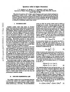
The numbers θ and ϕ define a point on the unit 3-dimensional sphere known as Bloch sphere (Fig. (2.1)). ,0 , z ,ψ , 2 y N x

,1 ,

Figure 2.1: Bloch sphere representation of a qubit |ψi = cos θ2 |0i + eiφ sin 2θ |1i. It is a good idea to use a vector representation in problems where we know with certainty the initial state of the qubit. An example of this statement is to prepare a qubit in the state |Ψi =

|0i+|1i √ , 2

that is, an equally weighted superposition of the canonical basis {|0i, |1i}.

However, let us consider a different scenario in which a qubit |Ψi is initially prepared in one of the following quantum states: {|ψi1 , |ψi2 , |ψi3 , . . . , |ψin } where each of the states is selected with probability

1 n.

We do not know what state was chosen to prepare |Ψi, but we do know that only

preparations |ψii , i ∈ {1, 2, . . . , n} are allowed. In this case, a convenient representation for |Ψi is n P |ψik k hψ|. the associated density operator ρˆΨ = n1 k=1

20


2.2.2

Evolution of a closed quantum system

Postulate 2 (Unitary operator version). The evolution of a closed quantum system with state ˆ (Def. (2.1.10)). The state of a system at vector |Ψi is described by a unitary transformation U time t2 according to its state at time t1 is given by

ˆ |Ψ(t1 )i. |Ψ(t2 )i = U

(2.9)

Postulate 2 only describes the mathematical properties that an evolution operator must have. The specific evolution operator required to describe the behaviour of a particular quantum system depends on the system itself. In the case of single qubits, any unitary operator can be realised in physical systems [137]. Postulate 2 can also be stated with the famous Schr¨ odinger equation. Postulate 2 (Hermitian operator version). The evolution of a closed quantum system is described by the Schr¨ odinger equation

i~

d|ψi ˆ = H|ψi dt

(2.10)

ˆ is a fixed Hermitian operator (Eq. (2.1.8)) known as the where ~ is Planck’s constant and H ˆ represent two ˆ and H Hamiltonian of the closed system (note that in spite of similar notation, H different things, being the former the Hamiltonian of Postulate 2 and the latter the Hadamard operator). The Hamiltonian of particular physical systems must be determined and calculated for each case. In general, figuring out the Hamiltonian of a particular physical system is a difficult task. In this thesis we make extensive use of the Hadamard operator (Eq. (2.4)) as evolution operator, among others. The effect of the Hadamard operator as evolution operator is exemplified in the following two equations: 1 1 ˆ H|0i = √ [|0ih0| + |0ih1| + |1ih0| − |1ih1|]|0i = √ (|0i + |1i) 2 2 1 1 ˆ H|1i = √ [|0ih0| + |0ih1| + |1ih0| − |1ih1|]|1i = √ (|0i − |1i) 2 2

21


2.2.3

Quantum measurements

In quantum mechanics, measurement is a non-trivial and highly counter-intuitive process. Firstly, because measurement outcomes are inherently probabilistic, i.e. regardless of the carefulness in the preparation of a measurement procedure, the possible outcomes of such measurement will be distributed according to a certain probability distribution. Secondly, once a measurement has been performed, a quantum system in unavoidably altered due to the interaction with the measurement apparatus. Consequently, for an arbitrary quantum system, pre-measurement and postmeasurement quantum states are different in general. ˆ m }, Postulate 3. Quantum measurements are described by a set of measurement operators {M index m labels the different measurement outcomes, which act on the state space of the system being measured. Measurement outcomes correspond to values of observables, such as position, energy and momentum, which are Hermitian operators (Def. (2.1.8)) corresponding to physically measurable quantities. Let |ψi be the state of the quantum system immediately before the measurement. Then, the probability that result m occurs is given by

ˆ† M ˆ p(m) = hψ|M m m |ψi

(2.11)

and the post-measurement quantum state is

|ψipm = q

ˆ m |ψi M

† ˆ ˆm hψ|M Mm |ψi

.

(2.12)

† ˆ ˆ m must satisfy the completeness relation, i.e. P M ˆm Operators M Mm = I because that guarm P P ˆ† ˆ antees that probabilities will sum to one: m hψ|Mm Mm |ψi = m p(m) = 1.

Let us work out a simple example. Assume we have a polarized photon with associated polarization orientations ‘horizontal’ and ‘vertical’. The horizontal polarization direction is denoted by |0i and the vertical polarization direction is denoted by |1i. Thus, an arbitrary initial state for our photon can be described by the quantum state |ψi = α|0i + β|1i, where α and β are complex num-

22


bers constrained by the normalization condition |α|2 + |β|2 = 1 and {|0i, |1i} is the computational basis spanning H2 . ˆ 0 = |0ih0| and M ˆ 1 = |1ih1| and two meaNow, we construct two measurement operators M surement outcomes a0 , a1 . Then, the full observable used for measurement in this experiment is ˆ = a0 |0ih0| + a1 |1ih1|. According to Postulate 3, the probabilities of obtaining outcome a0 or M outcome a1 are given by p(a0 ) = |α|2 and p(a1 ) = |β|2 . Corresponding post-measurement quantum states are as follows: if outcome = a0 then |ψipm = |0i; if outcome = a1 then |ψipm = |1i.

2.2.4

Composite quantum systems

We now focus on the mathematical description of a composite quantum system, i.e. a system made up of several different physical systems. Postulate 4. The state space of a composite quantum system is the tensor product of the component system state spaces. - If we have n quantum systems expressed as state vectors, labeled |ψi1 , |ψi2 , . . . , |ψin then the joint state of the total system is given by |ψiT = |ψi1 ⊗ |ψi2 ⊗ . . . ⊗ |ψin . - Similarly, if we have n quantum systems expressed as density operators ρ1 , ρ2 , . . . , ρn then the joint state of the total system is given by ρT = ρ1 ⊗ ρ2 ⊗ . . . ⊗ ρn (in the absence of any knowledge of correlations). As an advance of the operations we shall perform on the following chapters let us show the ˆ ⊗2 be the tensor details of applying an evolution operator to a composite quantum system. Let H product of the Hadamard operator (Eq. (2.4)) with itself and let |ψi = |00i. Then

ˆ ⊗2 |ψi = 1 (|00ih00| + |01ih00| + |10ih00| + |11ih00| + |00ih01| − |01ih01| + |10ih01| − |11ih01| H 2 + |00ih10| + |01ih10| − |10ih10| − |11ih10| + |00ih11| − |01ih11| − |10ih11| + |11ih11|)|00i

1 = (|00i + |01i + |10i + |11i) (2.13) 2

23

2.3 Entanglement Reduced density operator

Let us suppose we have a density operator describing a composite quantum system C and we are interested in studying the properties of one subsystem of C (such a situation would happen, for example, if after creating a bipartite quantum system we had access to only one particle.) The description of such a subsystem is provided by the reduced density operator, defined by Definition 2.2.1. Let A, B be two physical systems whose state is described by a density operator ρAB . The reduced density operator for system A is defined as

ρA ≡ trB (ρAB ) where trB is the partial trace over system B. The partial trace is given by

trB (|α1 ihα2 | ⊗ |β1 ihβ2 |) ≡ |α1 ihα2 |tr(|β1 ihβ2 |) ≡ |α1 ihα2 |hβ2 |β1 i

2.3

Entanglement

Entanglement is a unique type of correlation shared between components of a quantum system. Entangled quantum systems are sometimes best used collectively, that is, sometimes an optimal use of entangled quantum systems for information storage and retrieval includes manipulating and measuring those systems as a whole, rather than on an individual basis. Quantum entanglement and the principle of superposition are the main concepts behind the power of quantum computation and quantum information theory. The concept of correlation is deeply rooted in every branch of science. A typical and simple example is the following experiment: let us suppose we have two balls, one white and one black, as well as two boxes. If we randomly put a ball in each box and then close both boxes, we need to perform only one experiment, that is, to open one box, in order to know which of the balls is in each box. In other words, by means of one measurement, namely opening one box and seeing which ball was stored in it, we obtain two pieces of information, namely the colour of the ball stored in both boxes.

24

2.3 Entanglement

The former experiment is an example of classical correlation. Quantum entanglement is also a kind of correlation, but one that is detected only in quantum phenomena. A good example of the difference between classical and quantum correlations would be correlations in canonically conjugate observables, such as position and momentum. Consider the following 2-particle state:

|Ψ− i =

|01i − |10i √ 2

(2.14)

Clearly, |Ψ− i lives in a four-dimensional Hilbert space. It can be seen, after some calculations, that it is impossible to find quantum states |ai, |bi ∈ H2 such that |ai ⊗ |bi = |Ψ− i, that is, |Ψ− i is not a product state of |ai and |bi. This is indeed a criterion to determine whether a quantum state is entangled or not, whether it is possible to express such a composite quantum state as a simple tensor product of quantum subsystems. Another example is the tripartite entangled GHZ state

|GHZi =

|000i + |111i √ 2

(2.15)

Again, it is not possible to find three quantum states |ai, |bi, |ci ∈ H2 such that |ai ⊗ |bi ⊗ |ci = |GHZi. Entanglement definition and quantification is an open research area. Currently it is known how to identify and quantify entanglement for two particles but for three or more particles the situation is far less straightforward and remains an active area of research. In this thesis we use entanglement as a resource for building quantum walks, i.e. we assume the existence of entangled quantum systems and use standard methods of entanglement quantification to create new models of quantum walks.

2.3.1

Measure of entanglement

In order to quantify the degree of entanglement of the quantum systems studied in this thesis, we shall employ the reduced von Neumann entropy measure. For a pure quantum state |ψi of P a composite system AB with dim(A) = dA and dim(B) = dB , let |ψi = di=1 αi |iA i|iB i, (d = P min(dA ,dB ), αi ≥ 0 and di=1 α2i = 1) be its Schmidt decomposition. Also, let ρA = trB (|ψihψ|)

and ρB = trA (|ψihψ|) be the reduced density operators of systems A and B respectively. The entropy

25

2.3 Entanglement

of entanglement E(|ψi) is the von Neumann entropy of the reduced density operator [25, 45, 137].

E(|ψi) = S(ρA ) = S(ρB ) = −

d X

α2i log2 (α2i ).

(2.16)

i=1

E is a monotonically-increasing function of the entanglement present in the system AB. A nonentangled state has E = 0. States |ψi ∈ Hd for which E(ψ) = log2 d are called maximally entangled states in d dimensions. In particular, note that for those quantum states described by Eqs. (6.3a), (6.3b) and (6.3c) E(|Φ+ i) = E(|Φ− i) = E(|Ψ+ i) = 1, i.e. these states are maximally entangled.

2.3.2

Bell inequalities

We shall use Bell inequalities for entanglement detection in chapter 8, so in this subsection we discuss some of the main concepts behind those inequalities. This subsection is not meant to be either a complete or a thorough analysis of EPR arguments and Bell inequalities. Instead, our purpose is to give a brief introduction to this topic for non-physicists as well as to Bell inequalities’ potential use in applications of quantum computation. The counter-intuitive properties of quantum mechanics have always been a source of controversy. In their seminal paper [59], A. Einstein, B. Podolsky and N. Rosen (EPR) proposed a thought experiment with which they tried to show that quantum mechanics was an incomplete theory of Nature. The thought experiment proposed in [59] was developed under the following lines of thought:

1. Assumption of Realism. Physical properties have definite values which exist independent of observation. 2. Assumption of Locality. The description of a system’s state depends only in itself and its immediate surroundings. Therefore, for sufficiently separated physical systems, measurements performed on one of them cannot have any influence on the others.

These two assumptions together are known as local realism. According to [59], quantum mechanics was an incomplete theory under a local realistic description of Nature.

2.3 Entanglement

26

The discussion about the controversial properties of quantum mechanics shown in [59] was considered to be just philosophical for long time. However, in 1964 J. Bell published [17], in which he derived an inequality (involving correlated measurement results) that would have to be obeyed by any system behaving under the rules of local realism. Furthermore, it was also shown that for some entangled systems the inequality would be violated. Naturally, testing whether Nature was in fact local-realistic became an appealing idea. A number of experiments (page 12, [31]) have shown strong evidence that the inequality proposed in [17] is not obeyed by Nature4 . Furthermore, the quantum mechanical prediction was confirmed. The violation of Bell inequalities implies that at least one of the assumptions of local realism is in conflict with quantum mechanics. Although this is usually viewed as evidence for non-locality, there are some other possible explanations [31, 74]. In addition to its relevance to the foundations of physics, Bell inequalities can be used as a resource to detect entanglement in certain cases (for example, see [49, 164]). We shall elaborate more on this in chapter 8.

4

It must be noted that there is still controversy on the invalidity of local realism, at least in written evidence. For example, it was written on an essay by D. Bouwmeester and A. Zeilinger (page 12 of [31]) that “Even though a number of experiments have now confirmed the quantum predictions, from a strictly point of view the problem is not closed yet as some loopholes in the existing experiments still make it logically possible, at least in principle, to uphold a local realist world view”.

Chapter 3

Theory of Computation The purpose of this chapter is to present a concise introduction to the Theory of Computation, in order to provide the necessary background and to motivate our further discussion on the importance of classical random walks and quantum walks in computer science. We begin by providing an overview of the theory of computation and deliver a succint historical background of those ideas that led to its creation and development. We then formulate the essential concepts of a basic and yet powerful model of computation: Finite Automata. We use these concepts to introduce a formal definition of a model of computation that has played a most important role in the development of Computer Science: Turing Machines. We extend our discussion by introducing a third model of computation: Quantum Turing Machines. The previous concepts are followed by key definitions and theorems from Complexity Theory and the definitions of P, NP and NP-complete problem categories. This chapter is based on [52], [76], [142], [167] and [191].

3.1

What is the Theory of Computation?

The Theory of Computation is a scientific field devoted to understanding the fundamental capabilities and limitations of computers, and it is divided into three areas: 1. Automata Theory. The study of different models of computation. 2. Computability Theory. This focuses on determining which problems can be solved by computers and which cannot.

27

3.2 Hilbert’s program and the Entscheidungsproblem

28

3. Complexity Theory. The objective in this area is to understand what makes some problems computationally hard and other easy. The development of the theory of computation was driven in great part by several challenges posed by D. Hilbert and other mathematicians on the foundations of mathematics at the beginning of the 20th Century. A. Turing and other scientists, while working on the ideas required to formalize the idea of computation, answered some of the questions posed by Hilbert et al.

3.2

Hilbert’s program and the Entscheidungsproblem

At the beginning of the 20th century D. Hilbert and other mathematicians were aware that the methods of reasoning in mathematics could in some cases lead to contradictions. Hilbert believed that the proper way to develop any scientific subject rigorously required an axiomatic approach. In providing an axiomatic treatment, the theory would be developed independently of any need for intuition. Hilbert’s first step towards a rigorous formulation of mathematics was undertaken in his lecture at the International Congress of Mathematicians (Paris, 1900) [90], where he stated that “it shall be possible to establish the correctness of the solution by means of a finite number of steps based upon a finite number of hypotheses which are implied in the statement of the problem and which must always be formulated . . . This conviction of solvability of every mathematical problem is a powerful incentive to the worker. We hear within us the perpetual call: There is the problem. Seek its solution. You can find it by pure reason, for in mathematics there is no ignorabimus1 ”. The second step towards a rigorous formulation of mathematics was taken in 1920-1921, when Hilbert’s program was proposed [91]. Hilbert thought that, in order to formulate mathematics on a solid and complete logical foundation, it would suffice to prove that “all of mathematics follows from a correctly-chosen finite system of axioms, as well as that some such axiom system is provably consistent.” Finally, Hilbert and Ackerman posed a challenge known as the Entscheidungsproblem (Decision Problem) [92]. The Decision Problem is formulated in terms of first-order logic2 and can be stated as follows 1

Short for ignoramus et ignorabimus: we do not know and will not know. First-order logic or First Order Predicate Calculus (FOPC) is a formalisation of deductive logical reasoning. A concise tutorial on FOPC can be found in [52]. 2

3.3 On Computability

29

Definition 3.2.1. Entscheidungsproblem. Does there exist a procedure which can be followed for a finite number of steps in order to determine the validity of a given first-order statement? The idea of ‘finite procedure’ was deeply rooted in Hilbert’s proposals. A contemporary computer scientist would immediately think of an ‘algorithm’ as an equivalent definition of ‘finite procedure’. However, in Hilbert’s time the concept of algorithm did not exist yet. Alan Turing published a most influential paper in 1936 [175] in which he pionereed the theory of computation, introducing the famous abstract computing machines now known as Turing Machines. In [175], Turing explained the fundamental principle of the modern computer, the idea of controlling the machine’s operation by means of a program of coded instructions stored in the computer’s memory, i.e. Turing showed that it was possible to build a “Universal Turing Machine”, that is, a Turing machine capable of simulating any other Turing machine (the Universal Turing Machine being the actual digital computer and the simulated Turing machine the program that has been encoded in the digital computer’s memory). In addition, Turing proved that not all precisely stated mathematical problems can be solved by computing machines, in particular the Entscheidungsproblem. In the following section we deliver a brief summary of ideas and main results from [175].

3.3

On Computability

When Turing wrote [175], a computer was not a machine at all, but a human being. A computer was a mathematical assistant who calculated by rote, in accordance with a systematic method. The method was supplied by an overseer prior to the calculation. It is in that sense that Turing uses the word ‘computer’ in [175] and a Turing machine is an idealized version of this human computer. What Turing did in [175] was to propose a mathematical formalism for the idealization of a human computer as well as to study the calculation capabilites and limitations of that mathematical model. Turing meant by a systematic method (sometimes called an effective method and a mechanical method) any mathematical method for which all the following are true: 1. The method can, in practice or in principle, be carried out by a human computer working with paper and pencil. 2. The method can be given to a human computer in the form of a finite number of instructions.

3.4 Definition of a Problem and two examples

30

3. The method demands neither insight nor ingenuity on the part of the human being carrying it out. 4. The method will definitely work if carried out without error. Turing’s definition of a systematic method is the definition of an algorithm. Also, Turing proved that it was possible to build a particularly powerful machine called Universal Turing Machine (UTM) that could simulate any other Turing machine in reasonable time. Furthermore, Turing stated a conjecture now known as the Church-Turing Thesis, in which he established an equivalence correspondence between the existence of Turing machines and that of systematic methods. If the Church-Turing thesis is correct, then the existence or non-existence of systematic methods can be replaced throughout mathematics by the existence or non-existence of Turing machines. For instance, one could establish that there is no systematic method for doing a certain task by proving that no Turing machine can do the task in question. 3.3.1. The Church-Turing Thesis. Three ways to express the thesis are: 1. The UTM can perform any calculation that any human computer can carry out. 2. Any systematic method can be carried out by the UTM. 3. Every function which would be naturally regarded as computable can be computed by the Universal Turing Machine. Turing proved that it was not possible to build a Turing machine capable of solving problem from Def. (3.2.1), i.e. the Entscheidungsproblem is undecidable. If the Church-Turing thesis is true that means that the problem posed in Def. (3.2.1) cannot be solved by any algorithm, i.e. any finite method, as required by Hilbert. In this thesis we shall focus only on decidable problems, that is, problems for which it is possible to build Turing machines to solve them. In the following section we deliver some general properties of problems suitable to be solved by Turing machines, along with two relevant problems in Computer Science.

3.4

Definition of a Problem and two examples

We define a problem as a general question, usually possessing several parameters. A problem is specified by giving a general description of all its parameters, and a statement of what properties

3.4 Definition of a Problem and two examples

31

the solution is required to satisfy. An instance of a problem is obtained by specifying particular values for all the problem parameters. In general, we are interested in finding the “most efficient” algorithm for solving a problem, i.e. the fastest algorithm. The description of a problem instance is a finite string of symbols under a particular and reasonable encoding scheme, which maps problem instances into the strings describing them. To do this mapping we use the concept of language: Definition 3.4.1. Language. For any finite set of symbols Σ, we denote Σ∗ the set of all finite strings of symbols from Σ. If L ⊂ Σ∗ then L is a language over the alphabet Σ. For example, let Σ = {0, 1}. Then, Σ∗ = {φ, 0, 1, 00, 01, 10, 11, 000, 001, . . .} where φ is the empty string. Thus, L = {01, 001, 111, 10100101, 1111, 0001} is a language over Σ, as is the set of all binary representations of integers that are perfect cubes. The input length for an instance I of a problem ζ is the number of symbols in the description of I obtained from the encoding scheme of ζ. An algorithm solves a problem ζ if that algorithm can be applied to any instance I of ζ and is guaranteed always to produce a solution for that instance I. Two important problems in Computer Science are: Definition 3.4.2. The Traveling Salesman Problem INSTANCE: A finite set C = {c1 , c2 , . . . cm } of “cities” and a “distance” d(ci , cj ) ∈ N, the set of natural numbers. QUESTION: Which is the shortest “tour” of all the cities in C, that is, an ordering [cΠ(1) , cΠ(2) , . . . , cΠ(m) ] P of C such that [ m−1 i=1 d(cΠ(i) , cΠ(i+1) )] + d(cΠ(m) , cΠ(1) ) is minimum? Definition 3.4.3. The Satisfiability (SAT) Problem

Let S = {x1 , x2 , . . . , xn } be a set of Boolean variables. A truth assigment for S is a function t : S → {T, F }, for which if t(xi ) = T we say that xi is TRUE under t, and FALSE if t(xi ) = F . If xi is a variable under S then xi and x ¯i are literals over S. A clause over S is the disjunction of a set of literals over S (such as x1 ∨ x2 ∨ x ¯4 ) and it is satisfied by a truth assignment iff at least one of its members xi is true under that assignment. A collection C of clauses over S is satisfiable iff there exists some truth assignment for S that V W simultaneously satisfies all the clauses in C, i.e. C is a conjunction of disjunctions C = i [( j xj )].

3.5 Models of Computation and Algorithmic Complexity

32

Such a truth assigment is called a satisfying truth assignment for C. INSTANCE: A set S of variables and a collection C of clauses over S. QUESTION: Is there a satisfying truth assignment for C? In the theory of computation we usually work with decision problems, the reason being the need to build operational definitions of relevant problems. It is a matter of ingenuity to design a decision-problem version of a problem and it is not always the case that totally equivalent versions are obtained. Let us provide a decision-version of problem 3.4.2 as an example (note that the SAT problem (3.4.3) is already a decision problem). Definition 3.4.4. The Traveling Salesman Problem (Decision problem version) INSTANCE: A finite set C = {c1 , c2 , . . . cm } of “cities” a “distance” d(ci , cj ) ∈ N and a bound B ∈ N. QUESTION: Is there a “tour” of all the cities in C having total length no more than B, that is, an P ordering [cΠ(1) , cΠ(2) , . . . , cΠ(m) ] of C such that [ m−1 i=1 d(cΠ(i) , cΠ(i+1) )] + d(cΠ(m) , cΠ(1) ) ≤ B? We restrict ourselves to work with decision problems because languages, as defined in Def.

(3.4.1), are their natural counterpart, suitable to study in a mathematical fashion. The correspondence between decision problems and languages is brought about by the encoding schemes used to specify problem instances. An encoding scheme used describe each instance of a problem ζ partitions language Σ∗ into three classes of strings: strings that are not encoding of instances of ζ, those that encode instances of ζ for which the answer is ‘no’ and those that encode instances of ζ for which the answer is ‘yes’. Since we work with decidable problems, we are interested in the third class of strings. In the following section we present definitions and main results of three models of computation: Finite Automata, Turing Machines and Quantum Turing Machines.

3.5

Models of Computation and Algorithmic Complexity

Finite Automata, Turing Machines and Quantum Turing Machines are three models of computation. In this chapter, Finite Automata are presented and its results are used to introduce Turing machines; both models of computation are presented in their deterministic and nondeterministic versions.

33


Quantum Turing machines are introduced along with a physics-oriented version of the ChurchTuring thesis. Before introducing the above mentioned models, we will provide some concepts to quantify the amount of resources required to find an algorithmic solution to a problem.

3.5.1

Asymptotic Notation

The performance of models of computation in the execution of an algorithm is a fundamental topic in the theory of computation. Since the quantification of resources (in our case, we focus on time) needed to find a solution to a problem is usually a complex process, we just estimate it. To do so, we use a form of estimation called Asymptotic Analysis in which we are interested in the maximum number of steps Sm that an algorithm must be run on large inputs. We do so by considering only the highest order term of the expression that quantifies Sm . For example, the function F (n) = 18n6 + 8n5 − 3n4 + 4n2 − π has five terms, and the highest order term is 18n6 . Since we disregard constant factors, we then say that f is asymptotically at most n6 . The following definition formalises this idea. Definition 3.5.1. Big O Notation. Let f, g : N → R+ . We say that f (n) = O(g(n)) if ∃ α, no ∈ N such that ∀ n ≥ no f (n) ≤ αg(n) So, g(n) is an asymptotic upper bound for f (n) (“f is of the order of g”). Bounds of the form nβ , γ

β > 0 are called polynomial bounds, and bounds of the form 2n , γ ∈ R+ are called exponential bounds. f (n) = O(g(n)) means informally that f grows as g or slower. Big O notation says that one function is asymptotically no more than another. To state that one function is asymptotically no less than another we use the Ω notation. Definition 3.5.2. Ω Notation. Let f, g : N → R+ . We say that f (n) = Ω(g(n)) if ∃ α, no ∈ N such that ∀ n ≥ no g(n) ≤ αf (n) Finally, to say that two functions grow at the same rate we use the Θ notation.


34

Definition 3.5.3. Θ Notation. Let f, g : N → R+ . We say that f (n) = Θ(g(n)) if f (n) = O(g(n)) and f (n) = Ω(g(n)). Thus, f (n) = Θ(g(n)) means that f and g have the same rate of growth.

3.5.2

Deterministic Finite Automata

Deterministic Finite Automata is a model for computers with an extremely limited amount of memory. An example of a Deterministic Finite Automaton (DFA) is a machine R used to determine the parity of a sequence of characters like the one shown in Fig. (3.1). Suppose that R is at one of the ends of a wireless communication system. R can receive as valid input the characters ‘0’ and ‘1’, and, since any communication system is subject to errors, R can receive a third character ‘#’ which is used to state that an error has occurred in the transmission of the data stream. So, the input for R is an arbitrarily long set of characters (also known as a string) taken from the alphabet Σ = {0, 1, #}. The parity of a sequence of 0s and 1s is defined as follows: a sequence of 0s and 1s is odd if its number of 1s is odd, and it is even if its number of 1s is even. Let us now elaborate on the properties R must have. First, we state that only strings with no errors will be suitable for parity computation. Thus, only sequences of 0s and 1s will be accepted and any string has at least one error character must be rejected. Second, an empty set of characters has no 1s, thus we set the initial parity of a string as even. Let us show the behaviour of R with an example. Suppose that R receives as input the string 100110001 (read from left to right). The first input character is ‘1’ thus R goes from state ‘Even’ to state ‘Odd’. We then read ‘0’ and therefore we stay in state ‘Odd’. The third input character is again a ‘0’ and we remain in state ‘Odd’. As fourth input we receive a ‘1’ and then we move from state ‘Odd’ to state ‘Even’ as now we have an even number of ‘1’s in our account. The fifth input is a ‘1’ and consequently we move from state ‘Even’ to state ‘Odd’ as the total number of ‘1’s we have received so far is odd. The 6th , 7th and 8th characters are ‘0’ thus the current state of machine R remains being ‘Odd’. Finally, the last input character is ‘1’ and therefore R goes from state ‘Odd’ to state ‘Even’. The final outcome of the computation is the accept state ‘Even’. Formally speaking, a DFA is a list of five objects: set of states, input alphabet, rules for moving, start state, and accept states. We use a transition function to define the rules for moving. If the DFA has an arrow from state x to a state y labeled with the input symbol 1, that means that, if

35

3.5 Models of Computation and Algorithmic Complexity 1 0

0

Start

Odd 1

Even 0 1

#

#

Error 0,1,#

Figure 3.1: A finite automaton R for parity computation. Double-circled states are accept states and singlecircled state is a reject state. Input strings for R are taken from the set of any combination of characters taken from the alphabet Σ = {0, 1, #}.

the automaton is in state x when it reads a 1, it then moves to state y. We can indicate the same thing with the transition function by saying that δ(x, 1) = y. Definition 3.5.4. Deterministic Finite Automaton. A DFA R is a 5-tuple (Q, Σ, δ, qo , F ), where 1. Q is a finite set called the states, 2. Σ is a finite set called the alphabet, 3. δ : Q × Σ → Q is the transition function, 4. q0 ∈ Q is the start date, and 5. F ⊂ Q is the set of accept states. The formal description of the DFA R depicted in Fig. (3.1) is as follows: Q = {Even, Odd, Error}, Σ = {0, 1, #}, q0 = Even, F = {Even, Odd} and L(R) = {x ∈ {0, 1}n }. The transition function is given in Table 1. Table 1. Transition Function δ δ(Even, 0) = Even

δ(Even, 1) = Odd

δ(Even, #) = Error

δ(Odd, 0) = Odd

δ(Odd, 1) = Even

δ(Odd, #) = Error

δ(Error, 0) = Error

δ(Error, 1) = Error

δ(Error, #) = Error

Definition 3.5.5. Computation with a Deterministic Finite Automaton. Let R = (Q, Σ, δ, qo , F ) be a DFA and let w = w1 w2 . . . wn be a string where each wi is a member of the alphabet Σ. Then

36

3.5 Models of Computation and Algorithmic Complexity R accepts w if a sequence of states r0 , r1 , . . . , rn in Q exists with three conditions: 1. ro = q0 , 2. δ(ri , wi+1 ) = ri+1 , for i = 0, 1, . . . , n − 1, and 3. rn ∈ F .

Condition 1 means that the machine starts in the start state. Condition 2 states that the machine goes from state to state according to the transition function. Condition 3 says that the machine accepts its input if it ends up in an accept state. We say that R accepts language A if A = {w|R accepts w}, i.e. A is the set of all strings accepted by R.

3.5.3

Nondeterministic Finite Automata

When every step of a computation follows in a unique way from the preceding step (as in a DFA) we are doing deterministic computation. In a nondeterministic machine, several choices may exist for the next state at any point. Non determinism is a generalization of determinism, so every DFA is automatically a Nondeterministic Finite Automaton (NFA). Deterministic Computation Start

11 00 00 11 00 11

11 00 00 11 00 11

11 00 00 11 00 11 00 11

.. . 11 00 00 11 00 11

Reject

Non−deterministic Computation 00 11 00 11 0000000 01111111 1 00 00000011 111111 0000000 1111111 0 1 111111 000000 0000000 1111111 0 1 000000 111111 0000000 1111111 0 1 000000 111111 0000000 1111111 01111111 1 000000 111111 000 111 00 11 000 111 0000000 0 1 00000000 11111111 00000011 111111 000 111 00 000 111 00 11 00000000 11111111 0 1 00 11 00 11 00000 11111 000 111 00 11 000 111 00 11 00000000 11111111 0 1 00 11 00 11 00000 11111 0 1 00 1 11 00000000 11111111 0 00 11 00 11 00000 11111 0 1 00 11 00000000 11111111 0 1 00 11 00 11 00000 11111 0 1 00 11 00000000 11111111 0 1 0011 11 00 11 00000 11111 0 1 00 11 000 111 00 11 00 11 00000000 11111111 0 1 00 11 00 00 11 00000 11111 0 1 00 11 000 111 00 11 11 00 11 00 00000000 00 11 00 11 00 11 00 11 00 11 000 11111111 111 00 11 00 11 00 11 00 11 00 11 00 11 000 111 00 00 11 00 11 00 11 11 00 11

. . .

. ..

00 11 11 00 00 11

0 1 0 1 0 1 0 1 0 1 11 00 00 11 00 11 00 11 00 11 00 11 00 11 00 11 00 11 00 11 00 11 00 111 11 00 11 000 111 000 00 11 00 11 000 111 000 111 000 111 000 111 Accept 111 000 000 111

Reject

. . .

Accept

00 11 00 11 111 000 000 111 0 1 00 11 000 111 000 111 0 000 1 111 000 111 0 1 000 111 000 111 0 1 000 111 000 111 0 1 000 111 000 111 0 1 000 111 000 111 00 11 000 111 000 111 0 1 00 11 000 111 000 00 111 11 000 111 000 111

00 00 11 Accept 11 00 11 or Reject

Figure 3.2: In a DFA, every single step is fully determined by the previous step. In an NFA, a step may be followed by n new steps or, equivalently, an NFA makes n copies of itself, one for each possibility.

How does an NFA compute? Suppose that we are running an NFA on an input string and come to a state with multiple states to proceed. For example, say that we are in state qi in NFA N1


37

and that the next input symbol is 1. After reading that symbol, the machine splits into multiple copies of itself and follows all the possibilities in parallel. Each copy of the machine takes one of the possible ways to proceed and continues as before. If there are subsequent choices, the machine splits again. If the next input symbol does not appear on any of the arrows exiting the state occupied by a copy of the machine, that copy of the machine dies, along with the branch of the computation associated with it. Finally, if any one of these copies of the machine is in an accept state at the end of the input, the NFA accepts the input string. Another way to think of a nondeterministic computation is as a tree of possibilities. The root of the tree corresponds to the start of the computation. Every branching point in the tree corresponds to a point in the computation at which the machine has multiple choices. The machine accepts if at least one of the computation branches ends in an accept state. A graphical illustration of a nondeterministic computation is given in Fig. (3.2). An NFA is not a fully realistic model of computation as it assumes the capability of producing several instances of NFAs to run in parallel (it would be like suddenly producing as many computers as instances for each computation step). However, nondeterminism may be viewed as a kind of parallel computation wherein multiple independent processes can be running concurrently, and this view does prepare the grounds for introducing the concept of probabilistic computation, which will be reviewed in the following pages of this chapter. Definition 3.5.6. Nondeterministic Finite automaton. An NFA RN is a 5-tuple (Q, Σ, δ, qo , F ), where 1) Q is a finite set of states; 2) Σ is a finite alphabet; 3) δ : Q × Σ → P(Q) is the transition function; (P is the power set of set Q); 4) q0 ∈ Q is the start state, and 5) F ⊆ Q is the set of accept states. Definition 3.5.7. Computation on a Nondeterministic Finite Automaton. Let RN = (Q, Σ, δ, q0 , F ) be an NFA and w a string over the alphabet Σ. Then we say that RN accepts w if we can write w as w = y1 y2 . . . ym , where each yi is a member of Σ and a sequence of states r0 , r1 , . . . , rm exists in Q with three conditions: 1. r0 = q0 , 2. ri+1 ∈ δ(ri , yi+1 ), for i = 0, . . . , m − 1, and 3. rm ∈ F .

38


Condition 1 states that the machine starts out in the start state. Condition 2 means that state ri+1 is one of the allowable next states when N is in state ri and reading yi+1 . Observe that δ(ri , yi+1 ) is the set of allowable next states and so we say that ri+1 is a member of that set. Finally, condition 3 establishes that the machine accepts its input if the last state is an accept state. We say that RN accepts language A if A = {w|RN accepts w}, i.e. A is the set of all strings accepted by RN . It can be proved that DFAs and NFAs recognize the same class of languages [167]. However, the number of states of a deterministic counterpart of an NFA can be exponential in the number of branches of such an NFA and this is a very important difference between these two models of computation.

3.5.4

Deterministic Turing Machines

Similar to a DFA but with an unlimited and unrestricted memory, a Deterministic Turing Machine (DTM) is a much more accurate model of a general purpose computer. A DTM, pictured schematically in Fig. (3.3), can do everything a real computer can do.

Finite State Control Read−Write Head 1 0 0 1 0 1 0 1 0 1 0 1 0 1 0 1 0 1 0 1 0 1 0 1 0 1 0 1 0 1 0 1 0 1 0 1 0 1 0 1 0 1 0 1 0 1 0 1 0 1 0 1 0 1 0 1 0 1 0 1 0 1 0 1 0 1 0 1 0 1 0 1 0 1 0 1 0 1 0 1 0 1 0 1 0 1 0 1 0 1 11111111111111111111111111111111111111 00000000000000000000000000000000000000 11111 00000 0 1 0 1 0 1 0 1 0 1

...

...

−3

−2

−1

0

1

2

3

Figure 3.3: The ‘hardware’ elements of a Deterministic Turing Machine (DTM) are a limitless memory-type (the tape is divided into squares or cells), and a scanner which consists of read-write head plus a finite state control system. The scanner has two purposes: to read and write information on the cells of the tape as well as to control the state of the DTM. A DTM consists of a scanner and a limitless memory-tape that moves back and forth past the scanner. The scanner is composed of a read-write head as well as a finite state control system. The scanner does two tasks: it controls the state of the DTM through the finite state control system, and reads and writes information on the memory cells through the read-write head. The tape is divided into squares. Each square may be blank (t) or may bear a single symbol (0 or 1, for example). The


39

scanner is able to examine only one square of tape at a time (the ‘scanned square’). The scanner has mechanisms that enable it to write and erase the symbol on the scanned square, and to move the tape to the left or right, one square at a time. Also, the scanner is able to alter the state of the machine: a device within the scanner is capable of adopting a number of different states, and the scanner is able to alter the state of this device whenever necessary. The operations just described erase, print, move, and change state - are the basic operations of a DTM. Complexity of operation is achieved by chaining together large numbers of these simple basic operations. Note that according to the definitions of effective procedure and Turing machines, and under the assumption that the Church-Turing thesis holds, the concepts of Turing machine and algorithm are interchangeable. Definition 3.5.8. Deterministic Turing Machine. A Deterministic Turing Machine (DTM) is a 7-tuple M = (Q, Σ, Γ, δ, q0 , qaccept , qreject ), where Q, Σ, Γ are all finite sets and 1. Q is the set of states 2. Σ is the input alphabet not containing the blank symbol t, 3. Γ is the tape alphabet, where t ∈ Γ and Σ ⊂ Γ 4. δ : Q × Γ → Q × Γ × {L, R} is the transition function, 5. q0 ∈ Q is the start state, 6. qaccept ∈ Q is the accept state, and 7. qreject ∈ Q is the reject state, where qaccept 6= qreject . Definition 3.5.9. Computation with a Deterministic Turing Machine. Let M = (Q, Σ, Γ, δ, q0 , qaccept , qreject ) be a DTM. Initially M receives its input w ∈ Σ∗ on the leftmost n squares of the tape, and the rest of the tape is filled with blank symbols. The head starts on the leftmost square of the tape (Σ does not contain the blank symbol, so the first blank appearing on the tape marks the end of the input.) Once M has started, the computation proceeds according to the rules described by δ. The computation continues until it enters either the accept or reject states at which point it halts. If neither occurs, M just does not stop. As a DTM computes, changes occur in the current state, the current tape contents, and the current head location. A setting of these three items is called a configuration of the DTM. A


40

configuration C1 yields configuration C2 if the Turing machine can legally go from C1 to C2 in a single step. In an accepting configuration the state of the configuration is qaccept . In a rejecting configuration the state of the configuration is qreject . Accepting and rejecting configurations are halting configurations and do not yield further configurations. A DTM M accepts input w if a sequence of configurations C1 , C2 , . . . Ck exists, where 1. C1 is the start configuration of M on input w, 2. each Ci yields Ci+1 , and 3. Ck is an accepting configuration.

We say that M accepts language A if A = {w|M accepts w}, i.e. A is the set of all strings accepted by M . We show in appendix I how to use a DTM to recognize all numbers divisible by 4. We have said that DTMs can do everything a real computer can do, and real computers compute values of functions. Transducer Machines, a DTM variant, are capable of those computations. Definition 3.5.10. Transducer Machines. A transducer machine T is used to compute functions. T has a string w ∈ Σ∗ as input and produces another string y as output. Output y is stored in a special tape called the output tape. Given a function f , a transducer T computes f if the computation T (w) reaches a final state containing f (w) as output whenever f (w) is defined (if f is not defined, T never reaches a final state). A function f is computable if a Turing Machine T exists capable of computing it.

3.5.5

Algorithmic Complexity for DTMs

A DTM can be used to find a solution to a problem, so how efficiently can such a solution be found? As stated previously, we shall be interested in finding the fastest algorithms. Let us now introduce a few concepts needed to quantify the efficiency of an algorithm. The time complexity of an algorithm A expresses its time requirements by giving, for each input length, the largest amount of time needed by A to solve a problem instance of that size. Definition 3.5.11. Time Complexity Function for a DTM. Let M be a DTM. We define f : N → N as the time complexity function of M , where f (n) is the maximum number of steps that


41

M uses on any input of length n. Definition 3.5.12. Time Complexity Class for DTMs. Let t : N → R+ be a function. We define the time complexity class TIME(t(n)), as the collection of all languages that are decidable by an O(t(n)) time DTM. Definition 3.5.13. Class P. The class of languages that are decidable in polynomial time on a deterministic single-tape Turing machine is denoted by P and is defined as

P=

[

TIME(nk )

k

As an example, the language of appendix I is in P. A polynomial time or tractable algorithm is defined to be one whose time complexity function is O(p(n)) for some polynomial function p, where n is used to denote the input length. Any algorithm whose time complexity function cannot be so bounded is called an exponential time or intractable algorithm. Tractable algorithms are considered as acceptable, as a sign that a satisfactory solution for a problem has been found. Finding a tractable algorithm is usually the result of obtaining a deep mathematical insight into a problem. In contrast, intractable algorithms are usually solutions obtained by exhaustion, the so called brute-force method, and are not considered satisfactory solutions. For example, no tractable algorithm for the Travelling Salesman Problem (3.4.2) is known so far ([142] and [130]). All solutions proposed so far are based on enumerating all possible solutions. Why is the Travelling Salesman problem intractable? Nobody knows for sure. It could be either that we need a deeper knowledge of the characteristics of this problem or, simply, that the Travelling Salesman problem is inherently intractable. However, no proof for neither of these two alternatives has been supplied so far. DTMs are powerful machines. However, there are many decidable problems that require an unreasonable amount of resources from a DTM to be solved. In the following lines we introduce another model of computation used to tackle some of those problems. We shall study two of those problems in detail in the last part of this chapter, but before doing so we must introduce some formal definitions in order to have the tools required to define and attack


42

those problems.

3.5.6

Nondeterministic Turing Machines

The definition of a Nondeterministic Turing Machine (NTM) is similar to that of an NFA. The computation of an NTM is a tree whose branches correspond to different possibilities for the machine (see Fig. (3.2)). If some branch of the computation leads to the accept state qaccept then the machine accepts its input. Definition 3.5.14. Nondeterministic Turing Machine. A Nondeterministic Turing Machine is a 7-tuple MN = (Q, Σ, Γ, ∆, q0 , qaccept , qreject ), where Q, Σ, Γ are all finite sets, P(Q × Γ × {L, R}) is the power set of Q × Γ × {L, R}, and 1. Q is the set of states 2. Σ is the input alphabet not containing the blank symbol t, 3. Γ is the tape alphabet, where t ∈ Γ and Σ ⊂ Γ, 4. ∆ : Q × Γ → P(Q × Γ × {L, R}) is the transition relation, 5. q0 ∈ Q is the start state, 6. qaccept ∈ Q is the accept state, and 7. qreject ∈ Q is the reject state, where qaccept 6= qreject Notice that ∆ is not a function anymore but a relation, reflecting the fact that an NTM does not have a single, uniquely defined next action but a choice between several next actions. In other words, for each state and symbol combination, there may be more than one appropriate next step, or none at all. Definition 3.5.15. Computation with an NTM. An NTM MN accepts input w ∈ Σ∗ if at least one branch of its computation tree is a sequence of configurations C1 , C2 , . . . Ck such that 1. C1 is the start configuration of MN on input w, 2. each Ci yields Ci+1 , and 3. Ck is an accepting configuration. MN accepts language A if A = {w|MN accepts w}, i.e. A is the set of all strings accepted by MN . NTMs are powerful because of the assymetrical input-output relation found in the way these


43

machines compute. In order to have an NTM MN accept one string w it suffices to find just one branch b in the computation tree that accepts w. It can be shown that an NTM can be simulated by a DTM, i.e. that every NTM has an equivalent DTM ([167] and next section). However, simulating an NTM by a DTM may be at the cost of an exponential loss of efficiency [142]. Whether this loss is inherent to this ‘translation’ between models or is just a consequence of our limited understanding of nondeterminism is the ?

famous P = NP problem [142].

3.5.7

Algorithmic Complexity for NTMs

We start by offering the definitions of time complexity function and time complexity class for NTMs. Definition 3.5.16. Time Complexity Function for an NTM. Let MN be an NTM. We define g : N → N as the time complexity function of MN , where g(n) is the maximum number of steps that MN uses on any branch of its computation on any input length n. Definition 3.5.17. Time Complexity Class for NTMs. Let t : N → R+ be a function. We define the time complexity class NTIME(t(n)), as the collection of all languages that are decidable by an O(t(n)) time nondeterministic Turing machine. For an NTM to accept string w it is enough to find just one branch b in its computation tree that accepts w. However, a practical problem with this definition is to find b as an NTM can have an infinite (or exponentially big) number of different branches. Therefore, a more operational method for doing nondeterministic computation is needed. An important discovery in the theory of computation is the fact that the complexities of many problems are linked by means of a concept called verifiability. For example, let us suppose we have a proposed solution for the Travelling Salesman problem (3.4.4) and another solution for the SAT problem (3.4.3). In both cases, we could easily check whether each proposal is indeed a solution, all we need is a DTM that verifies whether proposed solutions are right or not. Let us formalize these concepts. Definition 3.5.18. Verifier. A verifier for a language A is an algorithm V , where


44

A = {w|V accepts (w, c) for some string c} We measure the time of a verifier only in terms of the length of w, so a polynomial time verifier runs in polynomial time in the length of w. A language A is polynomially verifiable if it has a polynomial time verifier. The string c, a certificate, is additional information needed by the verifier. For example, in the case of problem (3.4.4), c is the set of cities and distances, along with the bound B. In the case of the SAT problem (3.4.3), c is the actual clause collection to be tested. Note that a fundamental difference between an NTM (Def. (3.5.14)) and a verifier is that an NTM finds solutions, while a verifier only checks whether a proposal is a solution or not. We now proceed to define a most important class of languages in Computer Science: Definition 3.5.19. Class NP. The class of languages that have polynomial time verifiers is known as NP. What is the relation between the abstract model of an NTM and the concepts of verifiers and NP languages class? The answer is given in Theorem (4) and its proof can be found in [167]. Theorem 4. A language is in NP if and only if it is decided by a nondeterministic polynomial time Turing machine.

3.5.8

?

P = NP and NP-complete problems ?

The problem P = NP is a fundamental topic in the theory of computation. It is known that P ⊂ NP as any polynomial language can be checked with a polynomial verifier. Also, it can be proved [76] that Theorem 5. If a problem ζ ∈ NP then ∃ a polynomial p such that ζ can be solved by a deterministic algorithm having time complexity O(2p(n) ). Due to theorem (5) there is a widespread belief that P 6= NP although no proof has been ?

delivered and therefore P = NP remains an open problem.


45

There is a particular set of problems in NP that plays a key role in the theory of computation: NP-complete problems. In order to characterise this important set of problems we shall introduce the notion of polynomial transformations. Definition 3.5.20. Polynomial Transformation. A polynomial transformation from a language L1 ⊂ Σ∗1 to a language L2 ⊂ Σ∗2 , denoted by L1 ∝ L2 , is a function f such that 1. There is a polynomial time DTM that computes f . 2. ∀ x ∈ Σ∗1 , x ∈ Li ⇔ f (x) ∈ L2 Definition 3.5.21. NP-Complete Languages and Problems. A language L is NP-complete if L ∈ NP and, for all other languages Li ∈ NP we find that Li ∝ L. Due to our capacity to go from problem instances to languages by means of encoding schemes, we can also say that a decision problem ζ is NP-complete if ζ ∈ NP and, for all other decision problems ζi ∈ NP we find that ζi ∝ ζ. There is a plethora of NP-complete problems. The first NP-complete problem (chronologically speaking) was found by Stephen Cook ([50]) and it is stated in the following theorem (its proof can be found in [50] and [76]). Theorem 6. NP-Completeness of SAT problem. SAT problem is NP-complete. Therefore, studying the properties of SAT is an important and active area of research, not only because a polynomial-time solution to SAT would imply P = NP, but also because SAT is used to model problems and procedures in several areas of applied computer science and engineering like Artificial Intelligence (e.g. [77]) and hardware verification (e.g. [29] and [177]), using the following approach ([150]):

1. Represent the problem in propositional logic 2. Identify the proposition to be decided by satisfiability 3. Solve the SAT problem 4. Interpret the result in the original domain

3.6 Physics and the Theory of Computation

46

Surveys of algorithms for solving several variations and instances of SAT can be found in [77], [102] and [150] . Also, good introductions to the vast field of computational complexity can be found in [51], [72], [130], [141], and [167].

3.6

Physics and the Theory of Computation

Considerations about the physical properties of systems used to do computation and/or transmission of information have been studied for several decades. Consequently, physics and computer science have cross-fertilised each other for long time. As early as in the 1940s, in the beginning of the digital computer era, scientists wondered about the existence and quantification of the minimum amount of energy required to perform a computation. J. von Neumann, in a set of lectures delivered in 1949 [186], showed that “a minimum amount of energy required per elementary decision of a two-way alternative and the elementary transmittal of one unit of information” was close to kT , where k is Boltzmann’s constant and T is the temperature of the system. Later on, R. Landauer studied the relationship between energy comsumption and reversible computation (a computational step is reversible iff given the output of that step, its input is uniquely determined3 .) Among those results published by Landauer in [124] we have the following principle.

Landauer’s principle. Suppose a computer erases a single bit of information. The amount of energy dissipated into the environment is at least kT ln 2, where k is Boltzmann’s constant, and T is the temperature of the environment of the computer.

Landauer’s principle became a big motivation to do research in reversible computation. Among those works about reversible models of computation we find [24], [73] and [125]. Since evolution in quantum mechanics is reversible due to the use of unitary operators, the next step in the cross-fertilisation between computer science and physics was to link quantum mechanics and computer science. Benioff introduced the notion of Quantum Turing Machines and proposed a quantum mechanical model for the simulation of a classical computer ([19], [20], [21], [22] and chapter 6 of [66]). Additionally, R. Feynman, in his traditional and celebrated style, lectured at MIT 3

For example, the logical operation OR is not reversible, while the operation NOT is indeed reversible.


47

in 1981 [67] about the fundamental capabilities and limitations of classical computers to simulate quantum systems. A gentle and concise introduction to this blend of physics, computer science and information theory, as well as Feynman’s main ideas behind physics and computation can be found in [66]. In 1985 D. Deutsch made two key contributions in [53]: a design of a Universal Quantum Turing Machine, and a physics-oriented version of the Church-Turing thesis which he called ‘Church-Turing principle’:

The Church-Turing principle [53]. Every finitely realizable physical system can be perfectly simulated by a universal model computing machine operating by finite means.

In Deutsch’s words, the rationale behind the Church-Turing priciple was “to reinterpret Turing’s ‘functions which would be naturally regarded as computable’ as the functions which may in principle be computed by a real physical system. For it would surely be hard to regard a function ‘naturally’ as computable if it could not be computed in Nature, and conversely”. The Universal Quantum Turing machine proposed in [53] was further developed and improved by Yao [190] and Bernstein and Vazirani [28]. We now define a Probabilistic Turing Machine and a Quantum Turing Machine. Definition 3.6.1. [85] Probabilistic Turing Machine. A Probabilistic Turing Machine (PTM) is a Nondeterministic Turing Machine which randomly chooses between the available transitions at each point according to a probability distribution. Thus, a PTM MN = (Q, Σ, Γ, ∆, q0 , qaccept , qreject ), is a 7-tuple where Q, Σ, Γ are all finite sets, P(Q × Γ × {L, R}) is the power set of Q × Γ × {L, R}, and 1. Q is the set of states 2. Σ is the input alphabet not containing the blank symbol t, 3. Γ is the tape alphabet, where t ∈ Γ and Σ ⊂ Γ, 4. q0 ∈ Q is the start state, 5. qaccept ∈ Q is the accept state, and 6. qreject ∈ Q is the reject state, where qaccept 6= qreject


48

7. The transition relation is given by ∆ : Q × Γ → P(Q × Γ × {L, R} × [0, 1]), so that for a given configuration C0 , each of its successor configurations C1 , C2 , . . . , Cn is assigned a probability P p1 , p2 , . . . , pn , where n is the cardinality of P(Q × Γ × {L, R} × [0, 1]) and ni=1 pi = 1.

Definition 3.6.2. [85] Quantum Turing Machine. A Quantum Turing Machine is defined analogously to a PTM but with a different transition relation. The transition relation includes the use of complex numbers which are the corresponding amplitudes of quantum states used for computation. A QTM is a 7-tuple MN = (Q, Σ, Γ, ∆, q0 , qaccept , qreject ), where Q, Σ, Γ are all finite sets, P(Q × Γ × {L, R}) is the power set of Q × Γ × {L, R}, and 1. Q is the set of states 2. Σ is the input alphabet not containing the blank symbol t, 3. Γ is the tape alphabet, where t ∈ Γ and Σ ⊂ Γ, 4. q0 ∈ Q is the start state, 5. qaccept ∈ Q is the accept state, and 6. qreject ∈ Q is the reject state, where qaccept 6= qreject 7. The transition relation is given by ∆ : Q × Γ → P(Q × Γ × {L, R} × C[0,1] ), where C[0,1] ) = {z ∈ C| |z|2 ≤ 1}. So, for a given configuration C0 , each of its successor configurations C1 , C2 , . . . , Cn is assigned an amplitude z1 , z2 , . . . , zn , where n is the cardinality of P(Q × Γ × {L, R} × C[0,1] ) and Pn 2 i=1 |zi | = 1.

Quantum computation can be regarded as the study and development of methods that, by

using quantum mechanical properties, solve problems in finite time (from a different computational point of view, quantum computation is a sub-field of unconventional models of computation [38]). Quantum information can be defined as the field devoted to understanding how information is represented and communicated using quantum states. Due to the advances made over the last few years, both disciplines are now huge areas of research where diverse interests of several scientific communities can be found. Quantum walks is one of those interests, mainly contained in the sub-field of quantum algorithms.

Chapter 4

Classical Discrete Random Walks A stochastic process is a system which evolves in time while undergoing chance fluctuations. We can describe such a system with a family of random variables {Xt } where Xt measures, at time t, the property of the system which is of interest. Random walks, a particular type of stochastic processes, are relevant as mathematical entities, as well as in many other fields like physics and computer science [160]. In this thesis we are interested in comparing the statistical properties and computational applications of discrete random walks (i.e. classical random walks on discrete spaces in discrete time steps) with those of their quantum mechanical counterparts, quantum walks. To differentiate between discrete random walks and quantum walks, we will refer to the former as classical random walks and to the latter as quantum walks.

4.1

Probability theory and stochastic processes

In this section, based on [48], [82], [83], [138], [154] and [158], we provide some background results from probability theory and stochastic processes.

4.1.1

Discrete Random variables and distributions

Definition 4.1.1. Discrete Random Variable. An experiment is a situation with a set of possible outcomes. Let us suppose we have an experiment with outcome space E. A random variable (rv) is a real mapping X : E → R that is defined for all possible outcomes in 49

4.1 Probability theory and stochastic processes

50

S. A discrete random variable (drv) takes only a finite or countable infinite number of distinct values, i.e. X : E → A ⊂ R is a drv iff #(A) ≤ ℵ0 . The expression X = xi is shorthand for X(ei ) = xi , ∀ ei ∈ E, xi ∈ A. Definition 4.1.2. Probability distribution for a drv. Let X : E → A be a drv. Since the outcomes of an experiment are uncertain in general, we associate with each outcome xi ∈ A a probability p(xi ), where p(xi ) = Pr(X = xi ). The numbers p(xi ) are called a probability P distribution of X iff i) p(xi ) ≥ 0, and ii) xi ∈A p(xi ) = 1.

Definition 4.1.3. Expectation value and variance. The expectation value µ of a drv X, also P known as mean, is defined as E[X] = i xi p(xi ). More generally, the expectation value of any P function g(X) of X is given by E[f (X)] = i f (xi )p(xi ). The variance V [X] of a distribution, P also written as σ 2 , is given by V [X] = E[(X − µ)2 ] = i (xi − µ)2 p(xi ). The square root of the

variance is known as the standard deviation and is denoted by σ.

If X, Y are two drv and a, b ∈ R, the following propositions can be proved ([48]) E[aX + bY ] = aE[X] + bE[Y ]

(4.1)

V [X] = E[X 2 ] − (E[X])2

(4.2)

If X, Y are independent drvs ⇒ V [aX + bY ] = a2 V [X] + b2 V [Y ]

(4.3)

Definition 4.1.4. Bernoulli distribution. The Bernoulli distribution, denoted B(θ), is used as a model for experiments which have only two outcomes: success with probability θ, and failure with probability 1 − θ. If X is B(θ) then X = 1 if success and X = 0 if failure. It is a well known fact that if X is B(θ) then µX = θ and σ 2 = θ(1 − θ). Definition 4.1.5. Binomial distribution. The binomial distribution, denoted Bin(n, p), describes experiments that consist of a number of independent identical trials with two possible outcomes: success with probability p and failure with probability q = 1 − p. So, the random variable

51


X =‘number of successes’ can take any value from {1, 2, . . . , n} and its distribution is described by the binomial distribution. If X is Bin(n, p) then the probability p(r) of obtaining r successes from n trials is given by p(r) = nr pr q n−r .

Definition 4.1.6. Geometric distribution. The geometric distribution describes experiments that consist of a number of independent trials, each having a probability p, which are performed until a success occurs. If we let X be the number of trials required then the probability of getting a successful result after n trials is given by P (X = n) = (1 − p)n−1 p. If X is geometrically distributed then E[X] = 1p . Theorem 7. Markov’s inequality. Let X be a drv that takes only nonnegative values, then

P (X ≥ a) ≤ Proof. By Def. (4.1.3) E[X] =

P∞

i=1 xi p(xi )

E[X] = ≥ ≥

E[X] a

⇒

Pa−1 i=1

xi p(xi ) +

P∞

i=a xi p(xi )

P∞

= a

P∞

i=a xi p(xi )

i=a ap(xi )

P∞

i=a p(xi )

= aP (X ≥ a)

The mean and the variance of a drv X, although important quantities, do not contain all the information about the distribution of that variable1 . One way to completely characterize the probability distribution of a drv X is to use the moments of X.

4.1.2

Moments and generating functions

Definition 4.1.7. Moments of a drv. We define the kth moment of a drv X : E → A as µk = E(X k ) =

∞ X (xj )k p(xj ) j=1

1

It is possible to find two different probability distributions p1 and p2 corresponding to two different drvs X1 and 2 2 = σX . X2 with the same mean and variance, i.e. µX1 = µX2 and σX 1 2

52


where xi ∈ A, and under the assumption that the sum converges. It can be proved ([83]) that, in terms of its moments, the mean and the variance of a drv X are given by

µ = µ1

(4.4)

σ 2 = µ2 − µ21

(4.5)

Generating functions are a powerful and compact mathematical concept (power series) to encode information about sequences. In order to produce a moment generating function for a drv X, let us define the function

tX

e

=

∞ k X t k=0

Xk

(4.6)

etxj p(xj )

(4.7)

k!

By def. (4.1.3) we have

E(etX ) =

∞ X j=0

Thus

tX

E(e

∞ k ∞ k ∞ k X X X t t t k k X )= E(X ) = µk ) = E( k! k! k! k=0

k=0

k=0

Combining Eqs. (4.6) and (4.7) we obtain g(t) = E(etX ) =

∞ X

etxj p(xj ) =

j=0

∞ k X t k=0

k!

µk

Definition 4.1.8. Moment generating function. The function tX

g(t) = E(e

)=

∞ X

txj

e

p(xj ) =

j=0

is known as the moment generating function for X.

∞ k X t k=0

k!

µk

(4.8)

53

4.1 Probability theory and stochastic processes Theorem 8. Let g(t) be a moment generating function for drv X ⇒

Proof. By induction we find that

dn dtn g(t)

Since k(k − 1)(k − 2) . . . (k − (n + 1)) = We define αi =

(n+i)! i!(n+i)!

⇒

dn dtn

g(t)

dn g(t) dtn =

t=0

P∞

k=n

k! (k−n)!

"

= µn + t=0

= µn

⇒

k(k−1)(k−2)...(k−(n+1)) µk tk−n k!

dn dtn g(t)

=

P∞

i=n+1 αi µi t

i

P∞

k! k−n k=n (k−n)!k! µk t

#

= µn .

t=0

The binomial distribution is widely used in the study of classical random walks. In the following theorem we compute the moment generating function of a drv X Bin(n, p). Theorem 9. Let X be Bin(n,p) ⇒ gX (t) = (et p + q)n , with q = 1 − p Proof. By definition g(t) =

By the binomial theorem

P∞

txj p(x ) j j=0 e

Pn

⇒ gX (t) =

n tj j n−j j=0 j e p q

n tj j n−j . j=0 j e p q

= (et p + q)n .

Note that, if X is Bin(n, p) then d g(t) = net p(et p + q)n−1 = np, and µ2 = µ1 = dt t=0

Pn

d2 dt2

t=0

g(t)

t=0

= n(n − 1)p2 + np

Therefore, if a drv X is Bin(n, p) then its mean and variance are given by

µ = µ1 = np

(4.9a)

σ 2 = µ2 − µ21 = np(1 − p)

(4.9b)

The following theorem establishes the convergence and uniqueness properties of moment generating functions, and its proof can be found in [83].

54


Theorem 10. Let X be a drv with finite range {x1 , x2 , . . . xn }, distribution function p and moments µk ⇒ i) The moment series g(t) = g(t). ii) The moment series g(t) =

P∞

µk tk k!

converges for all t to an infinitely differentiable function

P∞

µk tk k!

is uniquely determined by p and conversely.

k=0

k=0

Finally with respect to generating functions, let us focus on the particular but important case in which a drv X takes values xj ∈ N ∪ {0}. In this case it is useful to have an alternative definition of a moment generating function. Definition 4.1.9. Ordinary generating functions. Let X : E → N ∪ {0} be a drv and g(t) be its P P∞ tj txj p(x ) = moment generation function. Since g(t) = ∞ j j=0 e j=0 e p(j) then g(t) is a polynomial

in et . Let us perform the variable change z = et and define the function h as

h(z) =

∞ X

p(j)z j

j=0

The function h(z) is called the ordinary generating function for X. Note that h(1) = g(0) = 1, h0 (1) = g0 (0) = µ1 and h00 (1) = g00 (0) − g0 (0) = µ2 − µ1 . An ordinary generating function is also simply called a probability generating function (pgf ). We use Def. (4.1.9) in the following result on Bernoulli distributions. Theorem 11. Let X be Bernoulli distributed with parameter θ ⇒ hX (z) = 1 − θ + θz. Proof. p(X = 0) = 1−θ and p(X = 1) = θ ⇒ h(z) =

P∞

j=0 z

j p(j)

= (1−θ)z 0 +θz 1 = 1−θ +θz.

Now we introduce another powerful mathematical tool to study classical random walks in both lines and graphs: Markov chains.

4.1.3

Markov chains

Definition 4.1.10. Markov chain. Let {Xα |α ∈ N ∪ {0}} be a set of discrete random variables and S be a system defined by the state space {sβ |β ∈ N ∪ {0}}. Xn is defined as the state of a system S at time n, so we say that S is in state si at time n iff Xn = si .


55

The sequence {Xα } is said to form a Markov chain with initial distribution λ and transition matrix P if each time S is in state si there is some fixed probability pij that it will be in state sj , and pij does not depend upon which states the chain was in before the current state. In other words,

P (Xn+1 = sj |Xn = sj−1 ∧ Xn−1 = sj−2 ∧ . . . X1 = s1 ∧ X0 = s0 ) = pij where the initial state s0 is drawn from the initial distribution λ. The values pij are called P the transition probabilities of the Markov chain and they satisfy pij ≥ 0 and i pij = 1, as

transition probabilities must conform a probability distribution. Transition matrices are also called

right stochastic matrices, i.e. matrices for which the sum of the elements of every and each row is equal to 1. The following lemma and theorem (corresponding proofs can be found in [83]) show the relationship between the time evolution of a Markov chain and its transition matrix P. Lemma 3. Let P be the transition matrix of a Markov chain. The ijth entry pnij of the matrix Pn gives the probability that the Markov chain, starting in state si , will be in state sj after n steps. − → Theorem 12. Let P be the transition matrix of a Markov chain, and let λ be the probability row vector which represents the initial distribution λ ⇒ the probability that the chain is in state si after − → n steps is the ith entry of the row vector λ (n) , given by − →(n) − → λ = λ Pn We now present an example of a stochastic system and its transition matrix. Example 4.1.1. Drunkard’s walk. A man is frequent visitor of a pub which is located 5 blocks from his home. If he is in any corner between home and the pub he walks to the left or to the right (i.e. towards home or the pub) with equal probability. Also, if he reaches either home or the pub he stays there. The behaviour of this man can be be modelled by a Markov chain with state space S = {1, 2, 3, 4, 5, 6}

56


being state s1 = 1 home and state s6 = 6 the pub, i.e. s0 and s5 are the absorbing states of this walk. The transition matrix is then 

       P=       

1

0

0

0

0



0   1/2 0 1/2 0 0 0     0 1/2 0 1/2 0 0    0 0 1/2 0 1/2 0    0 0 0 1/2 0 1/2    0 0 0 0 0 1

We are interested in studying several cases of Markov chains. A most important case is that in which it is possible to visit every state of the system S with no other constraint apart from the probabilities defined by the powers of the transition matrix P. The following definitions and theorems provide the grounds to characterise such Markov chains. Definition 4.1.11. Stationary probability distribution. Let P be a transition matrix. A → stationary probability distribution is a row vector − π that satisfies − → → π lim λ0 Pn = −

n→∞

Theorem 13. Let P be a transition matrix and π a stationary probability distribution ⇒ − → → π =− πP Definition 4.1.12. Irreducibility of a Markov chain. Let {Xα } be a Markov chain with state space S = {sβ } and transition matrix P. {Xα } is irreducible if ∀ si , sj ∈ S ∃ t ∈ N such that ptij > 0. So, a Markov chain is irreducible if it is possible to visit any state. In order to avoid any ‘visiting pattern’, we shall impose another condition on Markov chains, that of aperiodicity.

4.2 Classical random walks: results and applications

57

Definition 4.1.13. Periodicity of a Markov Chain. Let {Xα } be a Markov chain with state space S = {sβ } and transition matrix P. {Xα } is aperiodic if ∀si , sj ∈ S gdc{t ∈ N|ptij > 0} = 1 Definition 4.1.14. Ergodic Markov chains. A Markov chain is ergodic if it is irreducible and aperiodic. We are now ready to enounce a most important theorem of Markov chains. Theorem 14. Fundamental theorem of Markov chains [83]. An ergodic Markov chain has − → − → → a unique stationary distribution − π . For any initial probability distribution λ we have λ Pt → − → π as t → ∞.

So, if we let an ergodic Markov chain run for long enough, it will eventually lose all memory of → where it started and will reach some fixed distribution − π over its state space S = {sβ }. Therefore,

→ the unique stationary distribution − π of an ergodic Markov chain is independent of the initial − → probability distribution λ . This fact will be an important factor to differentiate between classical random walks and quantum walks.

4.2

Classical random walks: results and applications

The previous section will now be used to develop some important results of classical random walks on a line and on a graph. Those results will be employed in this thesis to present some applications of classical random walks in computer science, as well as to show the differences between this kind of stochastic processes and quantum walks (next chapter). Classical random walks were first thought as stochastic processes with no relation to algorithm development, thus besides to classical references on random walks like [56], [146] and [168], it is necessary to scan articles and a few books in order to find relevant material. Therefore, in addition to the references mentioned at the beginning of this chapter, we have used [127], [128] and [188] for this section.

58


4.2.1

Classical Random Walks on a Line

A classical random walk on a line is a particular kind of stochastic process. The simplest classical random walk on a line consists of a particle (“the walker”) jumping to either left or right depending on the outcomes of a probability system (“the coin”) with (at least) two mutually exclusive results, i.e. the particle moves according to a probability distribution. The generalisation to random walks on spaces of higher dimensions (graphs) is straightforward. An example of a random walk on a graph is a particle moving on a lattice where each node has 6 vertices, and the particle moves according to the outcomes produced by tossing a dice. In fact, a classical random walk on a line is also a random walk on a graph G(V, E) with |V | = 2. Classical random walks on graphs can be seen as Markov chains ([134] and [138].) Furthermore, if the random walk is aperiodic and irreducible then it has a stationary distribution (Theorem (14)). Unrestricted classical random walk on a line

. . . . . .

. . . −3

−2

−1

0

1

2

3

. . .

Figure 4.1: An unrestricted classical random walk on a line. The probability of going to the right is p and the probability of going to the left is q = 1 − p.

Let {Zn } be a stochastic process which consists of the path of a particle which moves along an axis with steps of one unit at time intervals also of one unit (Fig. (4.1)). At any step, the particle has a probability p of going to the right and q = 1 − p of going to the left. Compute the probability of finding the particle in position k after n steps. {Zn } has time parameter space N, discrete state space Z and the starting point is Z0 = 0. Each step is an independent drv X with distribution pr(X = 1) = p and pr(X = −1) = q. After n steps we can see that Zn =

n X

Xi

i=1

We are interested in finding the value Pkn = pr(Zn = k|Z0 = 0), so we define a new drv Yi

59


Each drv Yi =

1 2 (Xi

   1 if xi = 1; Yi =   0 if xi = −1

+ 1) is an independent Bernoulli trial (Def. (4.1.4)) with probability of

success p. We use {Yi } to define a drv Tn that represents the “number of successes” Tn =

n X k=1

1 Yi = (Zn + n) 2

Tn is Bin(n,p) (Def. (4.1.5)) ⇒ pr(Zn = k|Z0 = 0) = pr(Tn = 12 (Zn + n) = 21 (k + n)) ⇒

pr(Zn = k|Z0 = 0) =

   

n

1 (k+n) 2

  0,

1

1

p 2 (k+n) q 2 (n−k) ,

1 2 (k

+ n) ∈ N ∪ {0};

(4.10)

otherwise

Since Tn is Bin(n, p) then E[Tn ] = np and V [Tn ] = npq. So, using Eq. (4.1) we find

E[Zn ] = E[2Tn − n] = n(p − q)

(4.11)

V [Zn ] = V [2Tn − n] = 4npq. In other words, V [Zn ] = O(n)

(4.12)

Similarly, using Eq. (4.3)

Classical random walk on a line with two absorbing barriers We analize the case of the path of a particle which moves along a finite axis with steps of one unit at time intervals of one unit. The axis has absorbing boundaries −a and b, i.e. if the particle reaches either −a or b it remains there. As in the previous case, the particle has a probability p of going to the right and q = 1 − p of going to the left and each step is independent of every other step. Let {Zn } be the stochastic process that models the path of this particle, with time parameter space N and state space {−a, −a + 1, . . . , −1, 0, 1, 2, . . . , b − 1, b}. We are interested in computing the probability of Zn = −a before Zn = b (see Fig. (4.2)).

60


. . . −a

−a+1

−a+2

. . .

. . . −1

0

1

. . .

b−2

b−1

b

Figure 4.2: Classical random walk on a line with two absorbing barriers. The probability of going to the right is p and the probability of going to the left is q = 1 − p, except for the extreme sites in which the walker is absorbed with probability 1.

This problem is known as the Gambler’s ruin problem because one can think of it as two gamblers A and B with corresponding capitals of £a and £b. A and B play a game in which each play results in A winning £1 from B with probability p or B winning £1 from A with probability q. We want to know the probability that gambler A is in ruin. Let us define the drv

Yi =

   1 if A is eventually ruined, i.e. Zn = −a before Zn = b ;   0 otherwise

Y is B(θ) (Def. (4.1.4)), so the pgf of Y given that the walk starts in state i (Theorem (11)) is given by h(z)Y(i) = 1 − (1 − z)θi and we want to find θ0 , i.e. we want pr(Y = 1|Z0 = 0). Using techniques for solving difference equations, we find that

θ0 =

      

b a+b λb −1 λb −λ−a

λ=

p q

= 1;

λ=

p q

6= 1

(4.13)

Similarly, the probability that A is triumphant is given by

φ0 =

      

a a+b 1−λa 1−λa+b

λ=

p q

= 1;

λ=

p q

6= 1

(4.14)

We prove that the game will eventually end simply by showing that A will either lose or win with probability 1: θ0 + φ0 = 1.

61

4.2 Classical random walks: results and applications Classical random walk on a line with one absorbing barrier

This problem can be thought as a variation of the Gambler’s ruin problem, with gambler B having unlimited capital (B could be, for example, a casino). Therefore, we define a stochastic process {Zn } that models the path of a particle moving along an axis. Zn has time parameter space N and S state space {−a, −a + 1, . . . , −1, 0} N. As before, the particle has a probability p of going to the right and q = 1 − p of going to the left and each step is independent of every other step (see Fig.

(4.3)). We are interested in computing the probability pr(Zn = −a|Z0 = 0) This probability can be found by computing the limit

pr(Zn = −a|Z0 = 0) = lim θ0 = b→∞

   1

if p ≤ q;

  ( q )a p

(4.15)

if p > q

So, if B has unlimited capital and unless A has a success probability higher than that of his/her opponent, it is certain that A will be eventually ruined.

. . . a

a−1

a−2

. . .0

. . . 1

2

. . .

. . . b

b+1

. . .

Figure 4.3: Classical random walk on a line with one absorbing barrier. The walker can be absorbed in node a. The probability of going to the right is p and the probability of going to the left is q = 1 − p. In node a, the probability of being absorbed is equal to 1.

4.2.2

Classical random walks on a graph

A graph is a symbolic representation of a network and of its connectivity. Of particular importance in computer science is the relationship between graphs, Markov chains and classical random walks. Definition 4.2.1. Graph. A graph G = (V, E) is a set V of vertices vi connected by edges (vk , vl ) ∈ E. We define |V | as the total number of vertices and |E| as the total number of edges of G. The degree of a vertex is the number of edges of that vertex. A graph is connected if there is a path connecting every pair of vertices. A graph is bipartite if its set of vertices can be divided into two disjoint sets with two vertices of the same set never


62

sharing an edge, and non-bipartite otherwise. If ∀ (u, v) ∈ E ∃ (v, u) ∈ E ⇒ G is undirected. A graph can be represented by its adjacency matrix A = (aij ), which is a matrix with rows and columns labeled by graph vertices, with entries aij = 1 or 0 according to whether vertices i and j are linked by an edge or not. Graphs that encode the structure of a group are called Cayley graphs. Definition 4.2.2. Cayley graph. Let G be a finite group, and let S = {s1 , s2 , . . . , sk } be a generating set for G. The Cayley graph of G with respect to S has a vertex for every element of G, with an edge from g to gs ∀ g ∈ G and s ∈ S. Cayley graphs are k-regular, that is, each vertex has degree k. Cayley graphs have more structure than arbitrary Markov graphs and their properties are often used in algorithm development [103]. Graphs and Markov chains can be put in an elegant framework which turns out to be very useful for the development of algorithmic applications: Let G = (V, E) be a connected, undirected graph with |V | = n and |E| = m. G induces a Markov chain MG if the states of MG are the vertices of G, and ∀ u, v ∈ V

puv =

  

1 d(u)

  0

if (u, v) ∈ E; otherwise.

where d(u) is the degree of vertex u. Since G is connected, then MG is irreducible and aperiodic ([134]) therefore MG has a unique stationary distribution (Theorem (14)). Theorem 15. Let G be a connected, undirected graph with n nodes and m edges, and let MG be its corresponding Markov chain. Then, MG has a unique distribution − → π = (d(vi )/2m) → for all components vi of − π. Note that Theorem (15) holds even when the distribution {d(vi )} is not uniform. In particular, the stationary distribution of an undirected and connected graph with n nodes, m edges and constant → degree d(vi ) = r ∀ vi ∈ G, i.e. a Cayley graph, is − π = (r/2m), the uniform distribution.


63

We have established the relationship between Markov chains and graphs. We now proceed to define the concepts that make random walks on graphs useful in computer science. We shall begin by formally describing a random walk on a graph: let G be a graph. A random walk, starting from a vertex u ∈ V is the random process defined by s=u repeat choose a neighbour v of u according to a certain probability distribution P u=v until (stop condition) So, we start at a node v0 and, if at tth step we are at a node vt , we move to a neighbour of vt with probability given by probability distribution P . It is common practice to make Puv =

1 d(vt ) ,

where d(vt ) is the degree of vertex vt . Examples of random walks on graphs are a classical random walk on a circle or on a 3-dimensional mesh. We now introduce several measures to quantify the performance of random walks on graphs. These measures play an important role in the quantitative theory of random walks, as well as in the application of this kind of Markov chains in computer science. Definition 4.2.3. Hitting time. The hitting time Hij is the expected number of steps before node j is visited, starting from node i. Definition 4.2.4. Mixing rate. The mixing rate is a measure of how fast the random walk converges to its limiting distribution. The mixing rate can be defined in many ways, depending on the type of graph we want to work with. We use the definition given in [127]. If the graph is non-bipartite then ptij → dj /2m as t → ∞, and the mixing rate is given by (t) dj 1/t µ = lim sup max pij − t→∞ 2m

As is the case with the mixing rate, the mixing time can be defined in several ways. Basically, the notion of mixing time comprises the number of steps one must perform a classical random walk before its distribution is close to its limiting distribution.

64


Definition 4.2.5. Mixing time [10]. Let MG be an ergodic Markov chain which induces a → probability distribution Pu (t) on the states at time t. Also, let − π denote the limiting distribution of MG . The mixing time τ is then defined as → τ = max min{t|t ≥ T ⇒ ||Pu (t) − − π || < } u

t

→ where ||Pu (t) − − π || is a standard distance measure. For example, we could use the total variation P → distance, defined as ||Pu (t) − − π || = 21 i |Pui (t) − πi |. Thus, the mixing time is defined as the first → time t such that Pu (t) is within distance of − π at all subsequent time steps t ≥ T , irrespective of the initial state. Calculating mixing times is a difficult task. Consequently, there are several strategies to compute mixing times. Among them we find the coupling time strategy, which consists on considering two random walks on a Markov chain. By starting one of the random walks from the stationary distribution and bounding the time for the two chains to collide, we can compute bounds on the mixing time of the random walk. What does it mean to make two chains collide? That means that both chains will end up hitting the same nodes with the same probability. To formalise this concept, let us present the following theorem: (t)

Theorem 16. Let P and Q be two probability distributions with Px (t)

(t)

and Qx the probabilities of

(t)

hitting node x at time t ⇒ |P − Q| ≤ 2pr(Px 6= Qx ). So, the computation of the mixing time of a Markov chain by means of the coupling strategy consists of the following steps: 1. Compute the limiting distribution of the Markov chain. 2. (t)

Compute the time it takes to obtain the following equality: Px = πx , where πx is the probability → of hitting node x according to the Markov chain’s limiting distribution − π . This step is usually equivalent to computing the hitting time of the Markov chain for a certain node. The key question is: how many steps n does it take to hit node k? We now present the mixing times of several classical random walks.

65

4.2 Classical random walks: results and applications Mixing time of an unrestricted classical random walk on a line

It has been shown in Eq. (4.10) that, for an unrestricted classical random walk on a line with p = q = 12 , the probability of finding the walker in position k after n steps is given by

pr(Zn = k|Z0 = 0) =

Using Stirling’s approximation n! ≈

1 pr(Zn = k|Z0 = 0) = n 2

√

   

n

1 (k+n) 2

  0,

2πn

n n e

1 2n ,

1 2 (k

+ n) ∈ N ∪ {0};

otherwise

and after some algebra, we find

s n nn 2n ≈ n+k 1 π 2 (n2 − k2 ) (n + k) 2 (n − k) n−k 2 2 (k + n)

(4.16)

We know that Eq. (4.10) is a binomial distribution, thus it makes sense to study the mixing time in two different vertex populations: k p. 0.14

Probability of locating walker at position n


0.14

0.12

0.1

0.08

0.06

0.04

0.02

0 −100

−50

0 Position

50

100

0.12

0.1

0.08

0.06

0.04

0.02

0 −100

−50

0 Position

50

100

Figure 5.1: Probability distributions of 100 steps DQWLs using coin and shift operators given by Eqs. (5.1) and (5.2) respectively. Plot (a) corresponds to a DQWL with total initial quantum state |0ic ⊗ |0ip , while plot (b) had total initial quantum state |1ic ⊗ |0ip . Two interesting properties of these quantum walks is the skewness of corresponding probability distributions, along with the dependance of the symmetry of such skewness from the coin initial state.

2. Combinatorial approach. In this method we compute the amplitude for a particular position component |nip by summing up the amplitudes of all the paths which begin in the given initial condition and end up in |nip . This approach can be seen as using a discrete version of path integrals. In the following lines we review both approaches to analyse the Hadamard walk, a specific but very powerful DQWL with coin and shift operators given by Eqs. (5.1) and (5.2) respectively. Later on we show how the Hadamard walk is related to the more general case of a DQWL with arbitrary coin operator. Schr¨ odinger approach for the Hadamard walk The analysis of DQWL properties using the Discrete Time Fourier Transform (DTFT) and methods from complex analysis was first made by Nayak and Vishwanath ([136]), followed by Ambainis et al ([10]), Koˇs´ık [121] and Carteret et al ([40] and [41]). Following [10] and [136], a quantum walk ˆ )t |ψiinitial (Eq. (5.3)) or, alternatively, as on an infinite line after t steps can be written as |ψi = (U X k

[ak |0ic + bk |1ic ]|kip

(5.6)

where |0ic , |1ic are the coin state components and |kip are the walker state components. For

80

5.1 Quantum walk on a line example, let us suppose we have

|ψi0 = |0ic ⊗ |0ip

(5.7)

as the quantum walk initial state, with Eq.(5.1) and Eq.(5.2) as coin and shift operators. Then, the first three steps of this quantum walk can be written as: 1 1 |ψi1 = √ |0ic |1ip + √ |1ic | − 1ip , 2 2

1 1 1 1 |ψi2 = ( |0ic + 0|1ic )|2ip + ( |0ic + |1ic )|0ip + (0|0ic − |1ic )| − 2ip , 2 2 2 2 and

1 1 1 |ψi3 = ( √ |0ic + 0|1ic )|3ip + ( √ |0ic + √ |1ic )|1ip + 2 2 2 2 2 1 −1 ( √ |0ic + 0|1ic )| − 1ip + (0|0ic + √ |1ic )| − 3ip . 2 2 2 2 We now define 



ΨR (n, t) Ψ(n, t) =   ΨL (n, t)

(5.8)

as the two component vector of amplitudes of the particle being at point n and time t or, in operator notation

|Ψ(n, t)i = ΨL (n, t)|1i + ΨR (n, t)|0i

(5.9)

We shall now analyse the behaviour of a Hadamard walk at point n after t + 1 steps. We begin by applying the Hadamard operator given by Eq. (5.1) to those coin state components in position n − 1, n and n + 1:

81

5.1 Quantum walk on a line

ˆ H(|Ψ(n − 1, t)i + |Ψ(n, t)i + |Ψ(n + 1, t)i) =

1 √ (|ΨL (n − 1, t)i|0i + |ΨR (n − 1, t)i|0i − |ΨL (n + 1, t)i|1i + |ΨR (n + 1, t)i|1i 2 −|ΨL (n − 1, t)i|1i + |ΨR (n − 1, t)i|1i + |ΨL (n + 1, t)i|0i + |ΨR (n + 1, t)i|0i +|ΨL (n, t)i|0i + |ΨR (n, t)i|0i − |ΨL (n, t)i|1i + |ΨR (n, t)i|1i)

(5.10)

Now, we apply the shift operator given by Eq. (5.2) to Eq. (5.10)

ˆ (H(|Ψ(n ˆ U − 1, t)i + |Ψ(n, t)i + |Ψ(n + 1, t)i)) =

1 √ (|ΨL (n, t)i|0i + |ΨR (n, t)i|0i−|ΨL (n, t)i|1i + |ΨR (n, t)i|1i 2 −|ΨL (n − 2, t)i|1i + |ΨR (n − 2, t)i|1i + |ΨL (n + 2, t)i|0i + |ΨR (n + 2, t)i|0i −|ΨL (n − 1, t)i|1i + |ΨR (n − 1, t)i|1i + |ΨL (n + 1, t)i|0i + |ΨR (n + 1, t)i|0i) (5.11)

The bold font amplitude components of Eq. (5.11) are the amplitude components of |Ψ(n, t+1)i, which can be written in matrix notation as 

Let us label

Ψ(n, t + 1) = 

0



0

−1  √2

Thus

M =





√1 2

−1  √2

0

0  Ψ(n + 1, t) + 



√1 2

0

√1 2



0  and M+ = 

√1 2



0  Ψ(n − 1, t)

√1 2

(5.12)



0 

√1 2

Ψ(n, t + 1) = M Ψ(n + 1, t) + M+ Ψ(n − 1, t)

(5.13)

82


    1 0 Eq. (5.13) is a difference equation with Ψ(0, 0) =   and Ψ(n, 0) =  , ∀ n 6= 0 as initial 0 0

conditions (Eq. (5.7)).

The purpose of this analysis is to find analytical expressions for ΨL (n, t) and ΨR (n, t). To do so, we compute the Discrete Time Fourier transform of Eq. (5.13). The Discrete Time Fourier Transform is given by Definition 5.1.1. Discrete Time Fourier Transform. The Discrete Time Fourier Transform is part of the family of Fourier transforms. It transforms a function f (n) of a discrete “time” variable n ∈ Z into a continuous, periodic spectrum F (eiω ). Let f : Z → C be a complex function over the integers ⇒ its Discrete Time Fourier Transform (DTFT) f˜ : [−π, π] → C is given by ∞ X

iω

F (e ) =

f (n)e−inω ,

n=−∞

and its inverse is given by 1 f (n) = 2π

Z

π

F (eiω )einω dω

−π

Ambainis et al [10] use the following slight variant of the DTFT:

f˜(k) =

X

f (n)eik ,

(5.14)

n

where f : Z → C and f˜ : [−π, π] → C. Corresponding inverse DTFT is given by 1 f (n) = 2π

Z

π

f˜(k)e−ik dk

(5.15)

−π

So, using Eq. (5.14) we have

˜ Ψ(k, t) =

X n

Ψ(n, t)eikn

(5.16)

83

5.1 Quantum walk on a line Using Eq. (5.13) we obtain

˜ Ψ(k, t + 1) =

X (M Ψ(n + 1, t) + M+ Ψ(n − 1, t))eikn

(5.17)

n

After some algebra we get



−e−ik

e−ik

1  ˜ ˜ Ψ(k, t + 1) = Mk Ψ(k, t), where Mk = e−ik M + eik M+ = √  2 eik

eik

  

(5.18)

Thus 

   ˜ ΨL (k, t)  1 t˜ ˜ ˜ Ψ(k, t) =  0) , where Ψ(k, 0) =    = Mk Ψ(k, ˜ R (k, t) Ψ 0

(5.19)

Our problem now consists on diagonalising the (unitary) matrix Mk in order to calculate Mkt (Theorem (2)). If Mk has eigenvalues {λ1k , λ2k } and eigenvectors |Φ1k i, |Φ2k i then Mk = λ1k |Φ1k ih|Φ1k | + λ2k |Φ2k ihΦ2k |

(5.20)

Mkt = (λ1k )t |Φ1k ihΦ1k | + (λ2k )t |Φ2k ihΦ2k |

(5.21)

Using Def. (2.1.12) we find

It is shown in [136] and [10] that π π sin k λ1k = eiωk , λ2k = ei(π−ωk ) , where ωk ∈ [− , ] and sin(ωk ) = √ 2 2 2

(5.22)

and

Φ1k = q

1



e−ik



  √  √ 2eiωk + e−ik 2[(1 + cos2 (k)) + cos(k) 1 + cos2 k]

(5.23a)

84


Φ2k = q



1

e−ik



   √  p 2[(1 + cos2 (π − k)) + cos(π − k) 1 + cos2 (π − k)] − 2e−iωk + e−ik

(5.23b)

˜ L (n, t) From Eqs. (5.22), (5.23a) and (5.23b) we compute the Fourier-transformed amplitudes Ψ ˜ R (n, t) and Ψ −ik ˜ L (n, t) = √ e (eiωk t − (−1)t e−iωk t ) Ψ 2 1 + cos2 k

(5.24a)

cos k (−1)t ˜ R (n, t) = 1 (1 + √ cos k (1 − √ Ψ )eiωk t + )e−iωk t 2 2 1 + cos2 k 1 + cos2 k

(5.24b)

Using Eq. (5.1.1) on Eqs. (5.24a) and (5.24b), we prove the following theorem

Theorem 18. Let |Ψi0 = |0ip ⊗ |0ic be the initial state of a discrete quantum walk on an infinite line with coin and shift operators given by Eqs. (5.1) and (5.2) respectively ⇒ 1 ΨL (n, t) = 2π

ΨR (n, t) =

1 2π

Z

Z

π −π

−ieik √ (e−i(ωk t−kn) )dk 2 1 + cos2 k

π

−π

(1 + √

cos k )(e−i(ωk t−kn) )dk 2 1 + cos k

√ k ) and ωk ∈ [ −π , π ]. where ωk = sin−1 ( sin 2 2 2

The amplitudes for even n (odd n) at odd t (even t) are zero, as it can be inferred from the definition of the quantum walk. Now we have an analytical expression for ΨL (n, t) and ΨR (n, t), and taking into account that P (n, t) = |ΨL (n, t)|2 + |ΨR (n, t)|2 , we are interested in studying the asymptotical behaviour of Ψ(n, t) and P (n, t). Integrals in Theorem (18) are of the form 1 I(α, t) = 2π

Z

π

g(k)eiφ(k,α)t dk , where α = n/t( = position/number of steps)

−π

The asymptotical behaviour of this kind of integral can be studied using the method of stationary phase ([18] and [30]), a standard method in complex analysis. Using such a method, the authors of [10] and [136] reported the following theorems and conclusions:

85


−1 + , √12 − ). Then, as Theorem 19. Let > 0 be any constant, and α be in the interval ( √ 2

t → ∞, we have (uniformly in n) 2 π pL (n, t) v √ cos2 (−ωt + − ρ) , 2 4 π 1 − 2α t 2(1 + α) π √ cos2 (−ωt + ) 4 π(1 − α) 1 − 2α2 t √ √ 2α and ∆ = B 2 − 4(B + 1). where ω = αρ + θ, ρ = arg(−B + ∆), θ = arg(B + 2 + ∆), B = 1−α pR (n, t) v

√ √ Theorem 20. Let n = αt → ∞ with α fixed. In case α ∈ (−1, −1/ 2) ∪ (1/ 2, 1) ⇒ ∃ c > 1 for which pL (n, t) = O(c−n ) and pR (n, t) = O(c−n ). Conclusions 1. Quasi-uniform behavour. The wave function ΨL (n, t) and ΨR (n, t) (Theorem (18)) is almost √ √ uniformily spread over the region for which α is in the interval [−1/ 2, 1/ 2] (Theorem (19)), and shrinks quickly outside this region (Theorem (20)). Furthermore, by integrating the probability functions from Theorem (19), it is possible to see that almost all of the probability is concentrated √ √ in the interval [(−1/ 2 + )t, (1/ 2 − )t]. In fact, the exact probability value in that interval is P =1−

2 π

−

O(1) t .

2. Standard deviation. According to [136] and [10], the 0th and 2nd moments of the probability distribution from Theorem (19) are µ1 =

√ 1− √ 2 2

and µ2 =

√ 2−1 √ . 2

Being rigorous, and taking into

account that both moments were computed using normalised (over the total number of steps t) probability distributions, then the variance of the Hadamard walk is given by Eq. (4.5)

2 σH ˆ

= µ2 −

µ21

# "√ 2−1 √ t− = 2

"

√ # !2 1− 2 √ t 2

(5.25)

2 = O(t2 ) and, consequently, That is, σH ˆ

σHˆ = O(t)

(5.26)

86


However, the 2nd moment has also been interpreted ([110] and [115]) as the actual variance of the probability distribution given in Theorem (19). Furthermore, by introducing a novel method to compute the probability distribution X of the unrestricted DQWL, it was shown in [115] that q√ σ(X) 2−1 → as t → ∞. In any case, the standard deviation of the unrestricted Hadamard t 2 DQWL is O(t) and that result is in contrast with the standard deviation of an unrestricted classical √ random walk on a line, which is O( t) (Eq. (4.12)).

3. Mixing time. It was shown in [10] and [136] that an unrestricted Hadamard DQWL has a (q)

linear mixing time τ

(q)

= O(t), where t is the number of steps. Furthermore, τ

was compared

with the corresponding mixing time of a classical random walk on a line, which is quadratic, i.e. (c)

τ

= O(t2 ). In order to properly bound and evaluate the impact of this result in the fields of quantum walks

and quantum computation, a few clarifications are needed.

a) The mixing time measure used in this case is not the same as Eq. (4.2.5), the reason being that unitary Markov chains in finite state space (such as finite graph analogues of quantum walks) have no stationary distribution (section 2 of [10]). Instead, the mixing time measure proposed is given by Definition 5.1.2. Instantaneous Mixing Time.

τ = max min{t| ||Pu (t) − π|| ≤ } u

t

which is a more relaxed definition in the sense that it measures the first time that the current probability distribution Pu (t) is -close to the stationary distribution, without the requirement of continuing being -close for all future steps.

b) The stationary distribution of an unrestricted classical random walk on a line is the binomial distribution, spread all over Z. The only difference between Pt , the probability distribution of an


87

unrestricted classical random walk on a line at step t, and its limiting distribution P is the numerical value of the probability assigned to each node, as the shape of the distribution is the same. Although the binomial distribution can be roughly approximated by a uniform distribution for large values of t, depending on the precision we need for a certain task, that comparison is not precise. We can use the hitting time of an unrestricted classical random walk on a line together with Theorem (16) to figure out its corresponding mixing time. As shown in our chapter on classical random walks, the hitting time of an unrestricted classical random walk on a line depends on the √ region we are looking into. Specifically, the hitting time is O( t) for k t and O(2t ) for k ≈ t (Eqs. (4.17) and (4.18).) Thus, to hit node k with equal probabilities Ptk = Pk may depend on √ the region where k is located. For example, it may take O( t) if k t and O(2t ) if k ≈ t. As expressed in chapter 4, it seems that more analysis and new methods for studying mixing times on unrestricted classical random walks are required, particularly within the framework of algorithm development. So, comparing mixing times for quantum and classical unrestricted walks on a line is not necessarily clear and straightforward. Furthermore, and in order to reduce complexity in the analysis of algorithms, the infiniteness property of unrestricted classical random walks can sometimes be relaxed and properties of classical random walks on finite lines are used instead ([150]). This is indeed the case in the comparison of mixing times for classical and quantum walks on a line. As shown in Eq. (4.20), the hitting time (and therefore its mixing time) of a classical random walk on a line with reflecting barriers is O(t2 ), where t is the number of steps. Discrete Path Integral Analysis of the Hadamard Walk A different proposal to study the properties of quantum walks, based on combinatorics and the method given in [131] to quantify quantum state amplitudes, has been delivered in ([10], [40] and [41]). The main idea behind this approach is to count the number of paths that take a quantum walker from point a to point b. Thus, this approach can also be seen as a discrete path-integral method. Let us begin by stating the following lemma:

88

5.1 Quantum walk on a line Lemma 4. [10] and [131]. Let t ∈ [−n, n) ∩ Z and l =

t−n 2 .

The amplitudes of position n after t

steps of the Hadamard walk are: 1 X l−1 t−l √ (−1)l−k−1 ψL (n, t) = t k k 2 k 1 X l−1 t−l ψR (n, t) = √ (−1)l−k k 2t k k − 1

(5.27a)

(5.27b)

It was shown in [10] that the probabilities computed from those amplitudes of Lemma (4) can be expressed using Jacobi polynomials. Furthermore, it was shown in [41] that both Schr¨ odinger and combinatorial approaches are equivalent. (a,b)

Theorem 21. Let n ∈ N ∪ {0} and Jν (a,b)

in [], with Jν

(z) be the normalised degree ν Jacobi polynomial as defined

as its constant term. Let us also define ν =

(t−n) 2

− 1. Then

Pl (n, t) = 2−n−2 (Jν(0,n+1) )2 PR (n, t) =

t+n t−n

2

(5.28a)

2−n−2 (Jν(1,n) )2

(5.28b)

with

pL (−n, t) = pL (n − 2, t) and pR (−n, t) =

t−n t+n

2

pR (n, t)

A slight variation of this approach is given in [37]. An alternative method based on combinatorics and decompositions of unitary matrices has been proposed in [115], [116], [117] and [118]. Finally, Katori et al proposed in [101] the use of group theory to analyse symmetry properties of quantum walks on a line. Unrestricted DQWL with a general coin and with several coins The study of the Hadamard walk is relevant to the field of quantum walks not only as an example but also because of the fact that some important properties shown by the Hadamard walk (for example, its standard deviation and mixing time) are shared by any quantum walk on the line.

89

5.1 Quantum walk on a line In [171] it was shown that, for a general unbiased initial coin state

|ψ(x, 0)i =

√

η(|0ic + eiα

p

1 − η|1ic ) ⊗ |0ip

(5.29)

and a single step (in Fourier space) of the quantum walk ˜ t + 1)i = C˜k |ψ(k, ˜ t)i |ψ(k, where 

 C˜k =  √

√ ik ρe 1 − ρei(−k+φ)

√

ρei(θ+k)



1−  √ i(−k+θ+φ)  − ρe

(5.30)

is the Fourier transformed version of the most general 2-dimensional coin operator 

 C2 =  √

√ ρ 1 − ρeiφ

√

ρeiθ



1−  √ i(θ+φ)  − ρe

with θ, φ ∈ [0, π] and ρ ∈ [0, 1], we can express a t-step quantum walk on a line as 

˜ t + 1)i = C˜ t |ψ(k, ˜ 0)i, where |ψ(k, ˜ 0)i =  |ψ(k,  k

√



η   ⊗ |ki √ iα 1−η e

(5.31)

+ + t + ± ˜t If C˜k is expressed in terms of its eigenvalues λ± k and eigenvectors |λk i then Ck = (λk ) |λk ihλk |+ − t − (λ− k ) |λk ihλk |, and Eq. (5.31) can be written as

˜ 0)i ˜ 0)i + (λ− )t |λ− ihλ− |ψ(k, ˜ t + 1)i = (λ+ )t |λ+ ihλ+ |ψ(k, |ψ(k, k k k k k k

(5.32)

with r t (λ± 1 − η i(θ+α) √ i(k−δ) ∓iωk k ) −ik √ = e η− e ) , (5.33) e ( ρ∓e 1−ρ n± k q √ √ 2[1∓ ρ cos(k−δ∓ωk )] iδ e±iωk , n = where δ = (θ + φ)/2, sin(ωk ) = ρ sin(k − δ), λ± = ±e , k k 1−ρ t ± ˜ (λ± k ) hλk |ψ(k, 0)i

90


λ± = ±eiδ e±iωk and |λ± i =

1 n± k





eik

 

eiθ (λ± −

√

 . √ ρeik )/ 1 − ρ

As in the Hadamard walk case, the properties of the quantum walk defined by Eqs. (5.33) and (5.31) may be studied by inverting the Fourier transform and using methods of complex analysis. Let us concentrate on the phase factors α ∈ R of the coin initial state (Eq. (5.29)) and θ ∈ R of the coin operator (Eq. (5.30)). Note that we can choose many pairs of values (α, θ) for any phase factor r = α + θ. So, if we fix a value for θ (i.e. if we use only one coin operator) we can always vary the initial coin state |ψ(x, 0)i (Eq. (5.29)) to get a value for α so that we can compute a quantum walk with a certain phase factor value r. It is in this sense that we say that the study of a Hadamard walk suffices to analyse the properties of all unrestricted quantum walks on a line. In Fig. (5.2) we show the probability distributions of three Hadamard walks with different initial coin states.

0.12

0.07

0.1

0.08

0.06

0.04

0.02

0 −100

(a)

Hadamard walk Number of steps: 100. Initial conditions ((1/sqrt(2)|0>c +( i/sqrt(2)|1> c) ⊗ |o>p 0.08

Probability of locating walker at location n

Probability of finding walker at location n

Hadamard walk Number of steps: 100. Initial conditions ((1/sqrt(2)|0>c +( 1/sqrt(2)|1> c) ⊗ |o>p 0.14

−50

0 Position

50

0.06 0.05 0.04 0.03 0.02 0.01 0 −100

100

−50

(b)

0 Position

50

100

Hadamard walk Number of steps: 100. Initial conditions (sqrt(0.85)|0>c − sqrt(0.15)|1> c) ⊗ |o>p

Probability of finding walker at location n

0.08 0.07 0.06 0.05 0.04 0.03 0.02 0.01 0 −100

(c)

−50

0 Position

50

100

Figure 5.2: Graph (a) was computed√using coin √initial state |ψi0 = |0ic ⊗ |0ip . Graphs (b) and (c) had 1

|ψi = √2 (|0ic + i|1ic ) ⊗ |0ip and |ψi = 0.85|0ic − 0.15|1ic ) ⊗ |0ip as coin initial states, respectively. Notice that symmetry in the probability distribution can be achieved by using coin initial states with either complex or real relative phase factors [171]. All graphs were computed from 100-step Hadamard quantum walks on a line with Eq. (5.2) as shift operator.

The effect of different and multiple coins has been studied by several authors. In [97] and [135],


91

Konno and Inui have examined probability distributions computed with quantum walks on a line using 3 and 4 dimensional coins, respectively. The results shown in [97] have some similarities with those reported by the original contributions presented in chapter 6 of this thesis, in the sense that both quantum walks tend to concentrate most of their probability distributions about the origin of the walk (however, we show that in our case the probability distributions also have an important probability accumulation on the extremes.) Additionally, Ribeiro et al [152] have considered quantum walks with several biased coins applied aperiodically. In [37], Brun et al analysed the behaviour of a quantum walk on the line using both M 2-dimensional coins and single coins of 2M dimension. Furthermore, Ba˜ nulus et al [14] have studied the behaviour of quantum walks with a time-dependent coin, and Ermann et al [61] have inspected the decoherence of quantum walks with a complex coin, where the coin is part of a larger quantum system. More considerations on classical and quantum walks The links between classical and quantum versions of random walks have been studied by several authors. Watrous [187] studied how to simulate classical random walks using quantum systems. Some other authors have been interested in studying how quantum walks can become classical. For example, it was shown in [36] that such a transition could be achieved via two possible methods, in addition to the obvious procedure of performing measurements: decoherence in the quantum coin and the use of higher-dimensional coins. Moreover, by using a discrete path approach, it was shown in [118] that introducing a random selection of coins (that is, amplitude components for coin operators are chosen randomly, being under the unitarity constraint) makes quantum walks behave classically. In [42], the authors make use of a family of graphs (e.g. Fig. (5.5(a)) to exemplify the different behaviour of (continuous) quantum walks and classical random walks.) The “quantumness” of the quantum walk on a line has also been scrutinised. In [111] and [112] it was shown that it was possible to develop an implementation of a quantum walk on a line purely described by classical physics (wave interference of electromagnetic fields) and still be able to reproduce the variance enhancement which characterises that quantum walk. Kendon [107] showed it would still be necessary to have a quantum mechanical description of such an implementation in order to account for two properties of a quantum walk: the indivisibility of the

92


quantum walker and the trade-off between interference and information about the path followed by the walker. Furthermore and in an independent line of thought, Romanelli et al showed in [156] that the evolution equation of a quantum walk on a line can be separated into two parts: Markovian and interference terms, and that the quadratic increase in the variance of the quantum walker is a consequence of quantum evolution.

5.1.3

Quantum walk with boundaries

The properties of quantum walks on a line with one and two absorbing barriers were first studied in [10]. For the semi-infinite quantum walk on a line, Theorem (22) was reported Theorem 22. Let us denote by p∞ the probability that the measurement of whether the particle is at the location of the absorbing boundary (location 0 in [10]) ⇒ p∞ = π2 . Theorem (22) is in stark contrast with its classical counterpart (Eq. (4.15)), as the probability of eventually being absorbed is equal to unity. The case of a quantum walk on a line with two absorbing boundaries was also studied in [10], and their main result is given in Theorem (23). Theorem 23. For each n > 1, let pn be the probability that the process eventually exits to the left. Also define qn to be the probability that the process exits to the right. Then

i)∀ n > 1 ⇒ pn + qn = 1

1 ii) lim pn = √ n→∞ 2

Theorems (22) and (23) are revisited in [13] with (very detailed) corresponding proofs using both Fourier transform and path counting approaches. In addition, [13] proves some conjectures given in [189]. Finally, Konno studied the properties of quantum walks with boundaries using a set of matrices derived from a general unitary matrix together with a path counting method ([114] and [120]).

93

5.2 Quantum walks on graphs

5.2

Quantum walks on graphs

Classical random walks on graphs have been crucial to the development of stochastic algorithms [134]. In consequence, quantum walks on graphs has become an active area of research in quantum computation. A gentle introduction to the main ideas about discrete and continuous quantum walks on graphs, as well as to the quantification of resources required for their implementation, is given in [106]. Also, [129] presents numerical simulations of quantum walks in higher dimensions using separable and non-separable coin operators. In [4], Aharonov et al studied several properties of quantum walks on undirected graphs. Motivated by the importance of stationary distributions of Markov Chains (Theorem (14)), the quantum counterpart of a stationary distribution is studied in [4]. Their first finding consisted in proving that, if we use the classical definition of stationary distribution (Def. (4.1.11)), then quantum walks do not converge to any stationary state nor to any stationary distribution. In order to review the contributions of [4] and other authors, let us begin by formally introducing the following elements. Let G = (V, E) be a d-regular graph (Def. (4.2.1)) with |V | = n. Note that graphs studied in this section are finite, as opposed to the unrestricted line we used in the beginning of this chapter. Let Hv be the Hilbert space spanned by states |vi where v ∈ V . Also, we define HA , the coin space, as an auxiliary Hilbert space of dimension d spanned by the basis states ˆ the coin operator, as a unitary transformation in HA . Finally, label {|ii|i ∈ {1, . . . d}}, and C, each directed edge with a number between 1 and d so that the directed edges form a permutation (for Cayley graphs the labeling of a directed edge is simply the generator associated with the edge.) ˆ vi = |a, ui, where u is the ath neighbour Now, we define a shift operator Sˆ on Hv ⊗HA such that S|a, of v (since edge labeling is a permutation then Sˆ is unitary). Finally, we define one step of the ˆ = S( ˆ Cˆ ⊗ I). ˆ quantum walk on G as U As in the study of quantum walks on a line, if |ψi0 is the quantum walk initial state then a quantum walk on a graph G can be defined as

ˆ t |ψi0 |ψit = U

(5.34)

94


Before introducing the concept of quantum limiting distribution, we provide an example of a quantum walk on a graph: a discrete quantum walk on a cycle.

1 10

2

9

3

8

4 5

7 6

Figure 5.3: Quantum walk on a cycle. A cycle is a 2-regular graph which can be viewed as a Cayley graph of the group Z with generators 1, −1. The cycle shown in this figure has 10 vertices. Example. Discrete quantum walk on a cycle. Let Gcyc be a cycle with n nodes (see Fig. (5.3)). A quantum walk on Gc acts on a total Hilbert space H2 ⊗ Hn . For the sake of this example, we use the Hadamard coin operator given by Eq. (2.4) and the shift operator defined by ˆ ji = |0, j + 1 mod ni and S|1, ˆ ji = |0, j − 1 mod ni. S|0, Now, we discuss the definition and properties of limiting distributions for quantum walks on graphs. Suppose we begin a quantum walk with initial state |ψi0 . Then, after t steps, the probability distribution of the graph nodes induced by Eq. (5.34) is given by Definition 5.2.1. Probability distribution on the nodes of G. Let v be a node of G and Hd be the coin Hilbert space. Then

Pt (v|ψ0 ) =

X

i∈{1,...,d}

|hi, v|ψit |2

If probability distributions P0 , P1 at time 0 and 1 are different, it can be proved ([4]) that Pt does not converge. However, if we compute the average of distributions over time

95

5.2 Quantum walks on graphs Definition 5.2.2. Averaged probability distribution. T −1 1 X P¯t (v|ψ0 ) = Pt (v|ψ0 ) T t=0

We can obtain the following result ˆ . Then, Theorem 24. [4]. Let |ki, λk denote the eigenvectors and corresponding eigenvalues of U P for an initial state |ψi0 = k ak |ki lim P¯t (v|ψ0 ) =

t→∞

X

i,j,a

ai a∗j ha, v|iihj|a, vi

where the sum is only on pairs i, j such that λi = λj . ˆ are distinct, the limiting distribution takes a simple form. Let pi (v) = If all the eigenvalues of U 2 i∈{1,...,d} |hi, v|ki| ,

P

i.e. pi (v) is the probability to measure node v in the eigenstate |ki. Then it is P P possible to prove ([4]) that, for an initial state |ψi0 = k ak |ki ⇒ limT →∞ P¯t (v|ψ0 ) = i |ai |2 pi (v).

Using this fact it is possible to prove the following theorem.

ˆ be a coined quantum walk on the Cayley graph of an Abelian group, such Theorem 25. [4] Let U ˆ are distinct. Then the limiting distribution π (Def. (5.2.2)) is uniform that all eigenvalues of U over the nodes of the graph, independent of the initial state |ψi0 . Using Theorem (25) we compute the limiting distribution of a quantum walk on a cycle: Theorem 26. The limiting distribution π for the coined quantum walk on the n-cycle, with n odd, and with the Hadamard operator as coin, is uniform on the nodes, independent of the initial state |ψi0 . Several other important results for quantum walks on a graph are delivered in [4]. Among them, we mention some results on mixing times. Definition 5.2.3. Average Mixing time. The mixing time M of a quantum Markov chain with initial state |k, vi is given by M = min{T |∀t ≥ T ⇒ ||P¯t (k, v) − π(k, v)|| ≤ }

96


Theorem 27. For the quantum walk on the n-cycle, with n odd, and the Hadamard operator as coin, we have

M ≤ O(

n log n ) 3

So, the mixing time of a quantum walk on a cycle is O(n log n). The mixing time of corresponding classical random walk on a circle is O(n2 ) (Eq. (4.22)). Now we focus on a general property of mixing times. Theorem 28. For a general quantum walk on a bounded degree graph, the mixing time is at most quadratically faster than the mixing time of the simple classical random walk on that graph. The properties of the wave function of a quantum particle randomly walking on a circle have been studied in [69], and some details of limiting distributions of quantum walks on cycles are shown in [15] as well as in [16]. Also, the effect of using different coins on the behaviour of quantum walks on an n-cycle as well as in graphs of higher degree has been studied in [171]. Finally, a standard deviation measure for quantum walks on circles is introduced in [96]. Another graph studied in quantum walks is the hypercube, defined by Definition 5.2.4. The hypercube. The hypercube is an undirected graph with 2n nodes, each of which is labeled by a binary string of n bits. Two nodes ~x, ~y in the hypercube are connected by an edge if ~x, ~y differ only by a single bit flip, i.e. if |~x − ~y | = 1, where |~x − ~y | is the Hamming distance between ~x and ~y . As an example, the 3-dimensional hypercube is shown in Fig. (5.4). In [133], Moore and Russell derived values for the two notions of mixing times we have studied (Defs. (5.1.2) and (5.2.3)) for continuous and discrete quantum walks on the hypercube. As for the discrete quantum walk, [133] begins by defining Grover’s operator as coin operator. Definition 5.2.5. Grover’s operator. Let H be an n-dimensional Hilbert space and |ii be the Pn−1 ˆ = |ψihψ| − I. ˆ |ii. Then we define Grover’s operator as G canonical basis for H and |ψi = √1n i=0

97

5.2 Quantum walks on graphs Additionally, their shift operator is given by

Sˆ =

n−1 XX d=0 ~ x

|d, ~x ⊕ e~d ihd, ~x|

(5.35)

where e~d is the ith basis vector of the n-dimensional hypercube. So, the quantum walk on the hypercube proposed in [133] can be written as

ˆ t |ψi0 = [S( ˆG ˆ ⊗ Iˆn )]t |ψi0 |ψit = U

(5.36)

for a given initial state |ψi0 . Using a Fourier transform approach as in [136], it was proved in [133] that Theorem 29. For the discrete quantum walk defined in Eq. (5.36), its instantaneous mixing time (Def. (5.1.2)) is given by t =

kπ 4 n,

i.e. t = O(n), with = O(n−7/6 ) for all odd k.

[133] has several other contributions, and among those we would like to briefly mention that its authors elaborate on the fact that the relationship between different definitions of mixing times (i.e. instantaneous and average mixing times) for continuous and discrete quantum walks is not clear. Additionally, [133] provides analytical expressions for eigenvalues and corresponding eigenvectors of the evolution operator defined in Eq. (5.36) which were later used in [165] for the design of a search algorithm based on a discrete quantum walk (more on this in the next section). According to Theorem (28), the speedup that can be provided by a quantum walk on a graph is not enough to exponentially outperform classical walks. So, other parameters of quantum walks have been investigated, among them their hitting time. In [104], Kempe offers an analysis of hitting time of discrete quantum walks on the hypercube. Due to the fact that measurements destroy decoherence, two definitions of hitting time are proposed: Definition 5.2.6. One-shot hitting time. A quantum walk U has a (T,p) one-shot (|φ0 i, |xi) hitting time if the probability to measure state |xi at time T starting in |φi0 is larger than p, i.e. ||hx|U T |φ0 i||2 ≥ p.


98

Definition 5.2.7. |xi- stopped walk. A |xi-stopped walk from U starting in state |φ0 i is the ˆ0 = Π ˆ x = |xihx| and process defined as the iteration of a measurement with the two projectors Π ˆ 1 = Iˆ − Π ˆ 0 . If Π ˆ 1 is measured, an application of U follows. If Π ˆ 0 is measured the process is Π stopped. Definition 5.2.8. Concurrent hitting time. A quantum walk U has a (T,p) concurrent (|φ0 i, |xi) hitting time if the |xi-stopped walk from U and initial state |φ0 i has a probability ≥ p of stopping at a time t ≤ T . In both cases (Defs. (5.2.6) and (5.2.8)), it was shown in [104] that the hitting time from one corner to its opposite is polynomial. However, although it was thought that this polynomial hitting time would imply an exponential speedup over corresponding classical algorithms, that is not the case as it is possible to build a polynomial time classical algorithm to traverse the hypercube from one corner to its opposite [43]. Further studies on hitting times of quantum walks on graphs can be found in [122] and [123]. The sub-field of quantum walks on graphs is wide and rich. As a result, there are several interesting works which have not been covered in this thesis due to space restrictions. Briefly, we would like to mention the numerical simulations of quantum walks on graphs shown in [171], particularly the ‘localisation’ phenomenon due to the use of Grover’s operator (Eq. (5.2.5)) in a 2-dimensional quantum walk. Inspired by this phenomenon, Innui et al proved in [95] that the key factor behind this localisation phenomenon is the degeneration of the eigenvectors of corresponding evolution operator. In [80], Gottlieb et al studied the convergence of coined quantum walks in Rd . In [64], Feldman and Hillery have studied the relationship between quantum walks on graphs and scattering theory. Finally, L´ opez-Acevedo and Gobron [126] delivered an algebraic oriented analysis of quantum walks on Cayley graphs, while Montanaro presented in [132] a study on quantum walks on directed graphs.

5.3 Algorithmic applications of quantum walks

5.3

99

Algorithmic applications of quantum walks

A key field in quantum computation is the development of quantum algorithms. Since classical random walks have been used to develop stochastic algorithms, there has been a huge interest in understanding the properties of quantum walks over the last few years. A number of algorithms based on quantum walks are already known and we devote this section to review them. To do so, we introduce one more concept: oracles. Definition 5.3.1. Oracle. An oracle is an abstract machine used to study decision problems. It can be thought as a black box which is able to decide certain decision problems in a single step, i.e. an oracle has the ability to recognise solutions to certain problems. Oracles are widely used in classical algorithm design. In the context of quantum computation, we use oracles to recognise solutions for the search problem. Additionally, we assume that if an oracle recognizes a solution |φi then that oracle is also capable of computing a function with |φi as argument. We are interested in searching for M elements in a space of N elements. To do so, we use an index x ∈ S, where S = {0, 1, . . . , N − 1}, to number those elements. We also suppose we have a function f : S → {0, 1} such that f (x) = 1 if an only if x is one of the elements we are looking for. Otherwise, f (x) = 0. An oracle is a unitary operator O which can be defined by

O(|xi|qi) = |xi|q ⊕ f (x)i

(5.37)

where |xi is the index register, ⊕ is addition modulo 2 (the XOR operation in computer science parlance) and the oracle qubit |qi is a single qubit which is flipped if f (x) = 1 and is left unchanged otherwise. As shown in [137], we can check whether x is a solution to our search problem by preparing |xi, applying the oracle, and checking whether the oracle qubit has been flipped to |1i. Grover’s algorithm [84], as well as some of the algorithms we shall review in this section, make use of an oracle. A comparison of quantum oracles can be found in [100]. We now proceed to review quantum algorithms based on quantum walks. Even though this thesis is mainly devoted to discrete quantum walks, we shall briefly review an algorithm based on a continuous quantum walk, due to its relevance in the field.

100

5.3 Algorithmic applications of quantum walks 110

100

000

010 101

001

111

011

Figure 5.4: A 3-dimensional hypercube. Nodes are labeled following the formula d ⊕ ed where d ∈ {000, 001, 010, 011, 100, 101, 110, 111} and ed ∈ {001, 010, 100}. Exponential algorithmic speedup by a quantum walk In [63], E. Fahri and S. Gutmann introduced an algorithm based on a continuous quantum walk, i.e. a quantum walk whose evolution in time is not given in discrete steps, but it rather evolves continuously in time according to the Schr¨ odinger equation (Eq. (2.10)). The proposed algorithm solves the following problem: Given a graph Gs consisting of two balanced binary trees of height n with the 2n leaves of the left tree identified with the 2n leaves of the right tree according to the way shown in Fig. (5.5(a)), and with two marked nodes ENTRANCE and EXIT, find an algorithm to go from ENTRANCE to EXIT.

Entrance

Exit Entrance

(a)

Exit

(b) Figure 5.5: Balanced and unbalanced trees.

It was shown in [63] that it is possible to build a quantum walk that traverses graph Gs from ENTRANCE to EXIT which is exponentially faster than its corresponding classical random walk [42]. In other words, the hitting time (Def. (4.2.3)) of the continuous quantum walk proposed in [63] is of polynomial order, while the hitting time of the corresponding classical random walk is of

101


exponential order. However, this advantage does not lead to an exponential speedup due to the fact that it is possible to build a deterministic algorithm that traverses the same graph in polynomial time. Ideas from [63] were taken one step further by A. Childs et al in [43], where the authors introduced a more general type of graphs to be crossed, proved that those graphs could not be passed across efficiently with any classical algorithm, and delivered an algorithm based on a continuous quantum walk that traverses the graph in polynomial time. Graphs Gr are built as follows. Begin by constructing two balanced binary trees of height n (i.e. with 2n leaves), but instead of identifying the leaves, they are connected by a random cycle that alternates between the leaves of the two trees, that is, we choose a leaf on the left at random and connect it to a leaf on the right chosen at random too. Then, we connect the latter to a leaf on the left chosen randomly among the remaining ones. The process is continued, always alternating sides, until every leaf on the left is connected to two leaves on the right, and vice versa. See Fig. (5.5(b)) for an example of graphs Gr . In order to build the quantum walk that will be used to traverse a graph Gr , the authors of ˆ based on the graph adjacency matrix A (Def. (4.2.1)). H ˆ has matrix [43] defined a Hamiltonian H elements given by

ˆ ha|H|ai =

   γ, a 6= a0 , aa0 ∈ Gr   0,

(5.38)

otherwise

In the continuous quantum walk algorithm proposed in [43], the authors use an oracle to learn about the structure of the graph Gr , i.e. information about the Hamiltonian given by Eq. (5.38) is extracted using an oracle. By doing so, it is proved in [43] that it is possible to construct a continuous quantum walk that would traverse any graph Gr in polynomial time. An improved lower bound for any classical algorithm traversing Gr has been proposed in [65], but the performance difference between quantum and classical algorithms in [43] remains exponential.


102

Search algorithms based on quantum walks In order to review a series of quantum algorithms based on quantum walks, let us introduce the following problem: Definition 5.3.2. Searching in an unordered list. Suppose we have an unordered list of N items labeled x1 , x2 , . . . , xN . We want to find one of those elements, say xi . Any classical algorithm would take O(N ) steps at least to solve this problem. However, one of the jewels of quantum computation, Grover’s search algorithm [84], would do much better. By using an oracle and a technique called Amplitude Amplification, the search algorithm proposed √ in [84] would only take O( N ) time steps to solve the same search problem. In addition to its intrinsic value for outperforming classical algorithms, Grover’s algorithm has relevant applications in computer science, including solutions to the 3-SAT problem (Def. (3.4.3)) [8]. In [165], Shenvi et al proposed an algorithm based on a discrete quantum walk to solve the search problem given in Def. (5.3.2). [165] begins by using the eigenvalues and eigenvectors of ˆ of the quantum walk on the hypercube [133], in order to build a slightly the evolution operator U ˆ 0 . By collapsing the hypercube into a line, the quantum walk designed modified evolution operator U ˆ 0 is used to search for element xtarget ∈ {0, 1}n . It is claimed in [165] that, by evolution operator U √ √ ˆ 0 a number of tf = π 2n = O( N ) times, the outcome of their algorithm is xtarget after applying U 2 with probability

1 2

− O( n1 ). A summary of similarities and differences between this quantum walk

algorithm and Grover’s algorithm can be found in the last pages of [165]. A natural step further is to use quantum computation techniques to find items stored in spaces of 2 or more dimensions. In [23], Benioff proposed the use of Grover’s algorithm for searching items √ √ in a grid of N × N elements, and showed that a direct application of such algorithm would take O(N ) times steps to find one item, i.e. there would be no more quantum speedup. Later on, in [1] Aaronson and Ambainis used Grover’s algorithm and multilevel recursion to build algorithms √ capable of searching in a 2-dimensional grid in O( N log2 N ) steps and a 3-dimensional grid in √ O( N ) steps. Also, Childs and Goldstone [44] developed a continuous quantum walk algorithm to solve the search problem in a grid and discovered algorithms that would have an optimal performance √ of O( N ) in grids of 5 or more dimensions.


103

Ambainis et al proposed in [11] algorithms based on discrete quantum walks (evolution operators √ used in this paper are those ‘perturbed’ operators defined in [165]) that would take O( N log N ) √ steps to search in a 2-dimensional grid and would reach an optimal performance of O( N ) for 3 and higher dimensional grids. An important contribution of [11] was to show that the performance of search algorithms based on quantum walks is sensitive to the selection of coin operators, i.e. the performance of a search algorithm may be optimal or not depending on the coin operator choice. Finally, Aaronson and Ambainis have shown in [2] how to build algorithms based on discrete √ quantum walks to search on a 2-dimensional grid using a total number of O( N log5/2 N ) steps, √ and a 3-dimensional grid with O( N ) number of steps. A variant of Def. (5.3.2), the element distinctness problem, was analysed in [9]: Definition 5.3.3. Element distinctness problem [167]. Given a list of strings over {0, 1} separated by #, determine if all the strings are different. It was shown in [9] how to use discrete quantum walks to build algorithms to solve Def. (5.3.3) k

in a total number of O(N 2/3 ) steps and O(N k+1 ) steps for k different strings, among N items. A summary of quantum search algorithms can be found in [8], and a review of algorithmic applications of quantum walks can be found in [7].

Chapter 6

Quantum Walks and Entanglement I In this chapter we present a mathematical formalism for the description of unrestricted quantum walks with entangled coins and one walker. The numerical behaviour of such walks is examined when using a Bell state as the initial coin state, two different coin operators, two different shift operators, and one walker. We compare and contrast the performance of these quantum walks with that of a classical random walk consisting of one walker and two maximally correlated coins as well as quantum walks with coins sharing different degrees of entanglement. We illustrate that the behaviour of our walk with entangled coins can be very different in comparison to the usual quantum walk with a single coin. We also demonstrate that simply by changing the shift operator, we can generate widely different distributions. We also compare the behaviour of quantum walks with maximally entangled coins with that of quantum walks with nonentangled coins. Finally, we show that the use of different shift operators on 2 and 3 qubit coins leads to different position probability distributions in 1 and 2 dimensional graphs. This chapter is based on [179] Quantum Walks with Entangled Coins S.E. VenegasAndraca, J.L. Ball, K. Burnett and S. Bose New J. Phys. 7 221 (2005).

6.1

Introduction

In recent years interest in the field of quantum walks has grown hugely, motivated by the importance of classical random walks in computer science, as well as the advantages that quantum walks may

104

6.1 Introduction

105

provide us with when compared to their classical counterparts. Classical random walks are a fundamental tool in computer science due to their use in the development of stochastic algorithms [134]. In both theoretical and applied computer science, stochastic algorithms may outperform any deterministic algorithm built to solve certain problems. A notable example is that of the best algorithm known so far for the solution of 3-SAT (Def. (3.4.3)), a fundamental problem in computer science which relies on random walks techniques [93]. So, random walks are important elements of computer science. Additionally, the recent development of Quantum Computation and Quantum Information has revealed that the exploitation of inherently quantum mechanical systems for computational purposes leads to a number of significant advantages over purely classical systems. Thus it is reasonable to expect that the study of random walks using quantum mechanical systems may prove fruitful. As explained in chapter 5, a discrete quantum walk is composed of two physical systems: a walker and a coin. The properties of quantum walks applying multiple quantum coin operators ([37], [171] and [11]) as well as decoherent coins ([109], [110], [108] and [35]) on a single walker have been extensively studied (as a side comment, we mention that effects of quantum walker decoherence have also been studied for quantum walks on a line ([108] and [157]) and on the hypercube ([6]).) However, the use of entanglement in quantum walks is less well explored. A discussion on discrete quantum walks using non-separable evolution operators and its effects on the standard deviation of resulting probability distributions is given in [129], followed by [171] where a more exhaustive study on non-separable operators is provided. In [57], Du et al proposed an implementation of a continuous quantum walk on a circle, and numerically showed that entanglement in the position states shapes the position probability distribution. More recently, a discussion concerning models of a quantum walk on a line with two entangled particles as walkers is provided in [139]. A study of entanglement between coin and walker in quantum walks on graphs is given in [39], along with a generalization of the quantum walk algorithm from [43]. In [60] the authors analyse the relation between coin entanglement and the mean position of the quantum walker for 3 and 4 qubit coins. Finally, in [3], Abal et al have quantified the entanglement between walker and coin generated by the shift operator in a single coin-single walker quantum walk.

6.1 Introduction

106

Our motivation to use entangled coins in quantum walks comes from two sources. First, using entangled coins |ci ∈ Hn in quantum walks on graphs G(V, E) with deg(vi ) = m ∀vi ∈ V in which n > m, motivates the employment of different shift operators and therefore expands the dynamics of the quantum walk. In particular, in this chapter we use maximally entangled coins in quantum walks on an infinite line along with shift operators with “rest sites”, i.e. states that allow the walker to stay at the current vertex. Indeed, it is also possible to introduce pairs of coins in a classical random walk on an infinite line in order to expand its dynamics, but that is at the expense of varying the amount of correlation between the random variables produced with the outcomes of corresponding coins. Second, an entangled coin comprised of two qubits, each residing in H2 , can be viewed as a single coin defined on H4 , and then appropriately partitioned. Indeed the orthonormal basis {|00i, |01i, |10i, |11i} spans the space H4 . However, the phenomenon of entanglement represents a supercorrelation between possibly spacelike-separated subsystems of a total quantum system. It is certainly feasible to generate entanglement between two qubits and then separate them either for the purposes of an experiment in the laboratory, for example to allow for individual addressing of each qubit in some quantum information processing experiment (such as implementing the Hadamard operator), or to send them to opposite sides of the universe. This pre-existing entanglement resource is created during a finite time period of interaction and then the distinct subsystems can be separated to arbitrary locations. However, a single four-level quantum system cannot be physically broken and spatially separated into two pieces so that each piece is subsequently subjected to local operations. Partitioning a single coin into two entangled subsystems is nevertheless equivalent to using two distinct entangled coins, provided that the subsystems do not require to be physically separated for practical purposes. Although the mathematical description is the same, we choose to work with a pair of entangled qubits for two reasons: 1) we want to use a unique quantum property, i.e. entanglement, so that our model of quantum walks can be seen as a plausible model to possibly test the quantumness of quantum computers, and 2) we are interested in allowing experimentalists to address qubits globally or individually hen working with our proposal. Generation of photonic entangled states, for example by way of spontaneous parametric downconversion, or entangled states in ion traps, is already experimentally achievable. As such, identifying the entangled coins

6.1 Introduction

107

as bipartite states, rather than single and appropriately partitioned single system residing in H4 , is a natural choice to highlight and motivate possible links to experiment. Two specific physical implementations of quantum walks, namely cavity-QED based [162] and ion-trap based [170] motivate the scenario considered by us. In both these implementations, twolevel atoms serve as coins, while a cavity mode [162] or a vibrational mode [170] serve as the walker. Two atomic qubits in an ion trap are already feasible, and have been prepared in Bell states [159] and there are several proposals for entangling two atomic qubits in a cavity, such as [145]. These atoms can then be used as entangled coins with a common cavity mode or the common ion trap vibrational mode acting as the walker controlled by both these coins. While it is straightforward to treat the two atoms as individual qubits during this process, it is rather difficult to do entangling operations between them during the walk without using/affecting the cavity or vibrational mode which is already acting as the walker. Of course, a cavity mode or vibrational mode other than the one acting as walker may be used to do entangling gates between the atoms, but this is complicated. Moreover, in some cases, no method of accomplishing a direct unitary entangling gate between two atoms may be present, and their initial entanglement (needed for the walk considered here) may have been produced using other mechanisms (such as decays and measurements [145]). Because of this inherent difficulty of doing an entangling gate between the coins during a quantum walk, it is easier to imagine a scenario of two entangled coin qubits rather than a single four dimensional coin. Once two atoms have been trapped and entangled in a cavity, and this has already been done for ion traps, the implementation of our scenario is no more complex than a single coin quantum walk as the same global fields can be applied to both atoms for the coin and the shift operations (there is no need for addressing the atoms separately). In this chapter we shall discuss the behaviour of a quantum walk on an infinite line (also called unrestricted quantum walk) with one coin composed of two maximally entangled particles, and one walker. We compare the performance of such a walk with that of a classical random walk with one walker and two maximally correlated coins. We shall also study quantum walks with coins under different degrees of entanglement. Finally, we shall show that the use of different shift operators on 2 and 3 qubit coins leads to different position probability distributions in both one and two-dimensional graphs.

6.1 Introduction

108

The idea behind correlated coins is simple. For a pair of correlated coins C1 and C2 with corresponding outcomes (H1 , T1 ) and (H2 , T2 ) one expects that, after obtaining a certain outcome for coin C1 , coin C2 will produce its corresponding outcome according to a probability distribution defined by the degree of correlation between both coins. For example, the behaviour of a maximally correlated pair of coins would be the following: outcomes for coin C1 would be given according to a certain probability distribution. Let us suppose that coin C1 is unbiased, thus outcomes H1 and T1 may each occur with equal probability. Now let us suppose that we get H1 (T1 ) as outcome. Since the coin pair is maximally correlated, then the outcome for coin C2 will certainly be H2 (T2 ). If the degree of correlation were less than maximal between coins C1 and C2 , then obtaining outcome H1 for C1 would imply that the probability of getting H2 as outcome for coin C2 would not be unity. In fact the probability would scale as a monotonically increasing function of the degree of correlation between the coins. Using correlated coins in classical random walks is straightforward. For a classical random walk with a maximally correlated pair of coins it is natural to assign the walker one step to the right whenever the pair (H1 , H2 ) (say) is the resulting outcome, and one step to the left for the outcome (T1 , T2 ) (say). In this case, outcomes (H1 , T2 ) and (T1 , H2 ) have probability zero. Indeed, we could enrich our classical random walk by allowing coin outcomes O3 = (H1 , T2 ) and O4 = (T1 , H2 ). For example, one could use outcome O3 to permit the walker to remain in its current position or, alternatively, all four outcomes could be used to perform a random walk with 1 and 2 steps to the right and left, respectively. In particular, the introduction of outcomes that allow rest states is a feature used to remove the parity property of classical random walks, which consists of finding the walker only in even (odd) positions in an even (odd) time step. However, the introduction of outcomes O3 and O4 implies that the coin pair would no longer be maximally correlated. Our results show that probability distributions of quantum walks with maximally entangled coins have particular shapes that are highly invariant to changes in coin operators. These results are then compared with those obtained for classical random walks with maximally correlated coins.

6.2 Classical Random Walk with 2 Maximally Correlated Coins

109

This chapter is divided as follows. In the next section we formally introduce a classical random walk with a maximally correlated pair of coins. In Section 3 we present our results on unrestricted quantum walks on a line with a maximally entangled coin, followed by an analysis on quantum walks on a line using coins with different degrees of entanglement. The penultimate section of this chapter shows our simulation results on quantum walks with more than two maximally entangled coins and we finish this chapter with some conclusions.

6.2

Classical Random Walk with 2 Maximally Correlated Coins

A classical result from stochastic processes states that, for an unrestricted classical random walk starting at position z0 = 0, the probability of finding the walker at position k after n steps, when with probability p the walker takes a step to the right and with probability q = 1 − p takes a step to the left (i.e. tossing the coin with probability p of obtaining outcome T and probability q of obtaining outcome H), is given by

(n) Pok

=

1 1 n p 2 (k+n) q 2 (n−k) 1 2 (k + n)

(6.1)

for 21 (k + n) ∈ {0, 1, . . . , n} and 0 otherwise. Tossing a pair of coins produces two discrete random variables C1 and C2 , and the correlation ρ between these two random variables is given by ([82])

ρ(C1 , C2 ) = p

Cov(C1 , C2 ) Var(C1 )Var(C2 )

(6.2)

where Cov(X,Y ) and Var(X) are the covariance and the variance of the corresponding random variables. The function ρ is bounded by −1 ≤ ρ ≤ 1. ρ(C1 , C2 ) = 0 means that random variables C1 and C2 are totally uncorrelated (i.e. C1 and C2 are independent), whereas ρ(C1 , C2 ) = 1 means that random variables C1 and C2 are maximally correlated. The case ρ(C1 , C2 ) = −1 corresponds to perfect anticorrelation. Now consider a classical random walk that has a maximally correlated pair of coins, i.e. ρ(C1 , C2 ) = 1. Also suppose that the first coin C1 is unbiased. Then, as explained in the previous section, the

110

6.3 Quantum Walks with Entangled Coins

only two outcomes allowed for this coin pair are O1 = (H1 , H2 ) or O2 = (T1 , T2 ). If O1 allows the walker to move one step to the left and O2 allows the walker to move one step to the right, it is then clear that using such a coin pair in a classical random walk would produce a probability distribution equal to that of Eq. (6.1), with p = 21 . A plot of Eq. (6.1) with number of steps n = 100 and p =

1 2

is provided in Fig. (6.1) for the purpose of comparison with results presented in Section 3. 0.25

Probability of finding walker at position n

0.2

0.15

0.1

0.05

0 −100

(n) Figure 6.1: Plot of Pok =

−80

−60

−40

−20

0 Position

20

40

60

80

100

n

1 (k+n) 1 (n−k) q2 for n = 100 and p = 12 . The probability of finding the p2 walker in position k = 0 is equal to 0.0795. Only probabilities corresponding to even positions are shown, as odd positions have probability equal to zero. 1 2 (k+n)

As can be seen in Fig.(6.1), the use of maximally correlated unbiased coins in classical random walks is not different to a classical random walk with a single unbiased coin, as the probability distributions from both kinds of classical random walks are exactly the same. In the following sections we shall compare the results obtained by the computation of classical random walks with maximally correlated (classical) coins with those of quantum walks with maximally entangled (quantum correlated) coins.

6.3 6.3.1

Quantum Walks with Entangled Coins Mathematical Structure of Quantum Walks on an Infinite Line Using a Maximally Entangled Coin

As before, the elements of an unrestricted quantum walk on a line are a walker, a coin, evolution operators for both coin and walker, and a set of observables. We shall provide a detailed description of each element motivated by the previous subsection.

111


Walker and Coin: The walker is, as in the unrestricted quantum walk with a single coin, a quantum system |positioni residing in a Hilbert space of infinite but countable dimension HP . The P canonical basis states |iiP that span HP , as well as any superposition of the form i αi |iip subject P to i |αi |2 = 1, are valid states for the walker. The walker is usually initialised at the ‘origin’ i.e. |positioni0 = |0iP .

The coin is now an entangled system of two qubits i.e. a quantum system living in a 4dimensional Hilbert space HEC . We denote coin initial states as |coini0 . Also, we shall use the following Bell states as coin initial states 1 |Φ+ i = √ (|00i + |11i) 2

(6.3a)

1 |Φ− i = √ (|00i − |11i) 2

(6.3b)

1 |Ψ+ i = √ (|01i + |10i) 2

(6.3c)

which are maximally entangled pure bipartite states with reduced von Neumann entropy equal to unity. We shall examine the consequences of employing such maximally entangled states by comparing the resulting walks with those resulting from using maximally correlated coins in classical random walks. The Bell singlet state |Ψ− i =

√1 (|01i − |10i) 2

is not used as an entangled coin as the

singlet state remains the same when the same local unitary operator is applied to its constituent qubits. The total initial state of the quantum walk resides in the Hilbert space HT = HP ⊗ HEC and has the form |ψi0 = |positioni0 ⊗ |coini0

(6.4)

Entanglement measure: In order to quantify the degree of entanglement of the coins used in this chapter, we shall employ the reduced von Neumann entropy measure (Eq. (2.16)). Evolution Operators: The evolution operators used are more complex than those for quantum walks with single coins. As in the single coin case, the only requirement evolution operators must fulfil is that of unitarity.

112


Let us start by defining evolution operators for an entangled coin. Since the coin is a bipartite system, its evolution operator is defined as the tensor product of two single-qubit coin operators: CÊC = Cˆ ⊗ Cˆ

(6.5)

H as the tensor product H ˆ ⊗2 : For example, we could define the operator CÊC

1 H CÊC = (|00ih00| + |01ih00| + |10ih00| + |11ih00| + |00ih01| − |01ih01| + |10ih01| − |11ih01| 2 + |00ih10| + |01ih10| − |10ih10| − |11ih10| + |00ih11| − |01ih11| − |10ih11| + |11ih11|). (6.6) An alternative bipartite coin operator is produced by computing the tensor product Yˆ ⊗2 where Yˆ =

√1 (|0ih0| 2

+ i|0ih1| + i|1ih0| + |1ih1|), namely

1 Y CÊC = (|00ih00| + i|01ih00| + i|10ih00| − |11ih00| + i|00ih01| + |01ih01| − |10ih01| + i|11ih01| 2 + i|00ih10| − |01ih10| + |10ih10| + i|11ih10| − |00ih11| + i|01ih11| + i|10ih11| + |11ih11|). (6.7) Both coin operators are fully separable, thus any entanglement in the coins is due to the initial states used. The conditional shift operator SÊC necessarily allows the walker to move either forwards or backwards along the line, depending on the state of the coin. The operator

SÊC = |00icc h00| ⊗

X

|i + 1ipp hi| + |01icc h01| ⊗

+|10icc h10| ⊗

X

|iipp hi| + |11icc h11| ⊗

i

i

X i

X i

|iipp hi| (6.8)

|i − 1ipp hi|

embodies the stochastic behaviour of a classical random walk with a maximally correlated coin pair. It is only when both coins reside in the |00i or |11i state that the walker moves either forwards or backwards along the line; otherwise the walker does not move.

113


Note that SÊC is one of a family of valid definable shift operators. Indeed, it might be troublesome to identify a classical counterpart for some of these operators: their existence is uniquely quantum-mechanical in origin. One such alternative operator is 0 SÊC = |00icc h00| ⊗

+|10icc h10| ⊗

X i

X i

|i + 2ipp hi| + |01icc h01| ⊗

|i − 1ipp hi| + |11icc h11| ⊗

X i

X i

|i + 1ipp hi| (6.9)

|i − 2ipp hi|.

ˆT = SÊC .(CÊC ⊗Îp ) and a succint mathematical The total evolution operator has the structure U ˆT )N |ψi0 , where |ψi0 denotes the initial representation of a quantum walk after N steps is |ψi = (U state of the walker and the coin. H , C ˆ Y and In the rest of this chapter and for the sake of clarity, we shall use the symbols CÊC EC

SÊC to refer to Eqs. (6.6), (6.7) and (6.8), respectively. Observables: The observables defined here are used to extract information about the state of the ˆT )N |ψi0 . quantum walk |ψi = (U We first perform measurements on the coin using the observable

ˆ EC = β00 |00icc h00| + β01 |01icc h01| + β10 |10icc h10| + β11 |11icc h11|. M

(6.10)

Measurements are then performed on the position states using the operator ˆP = M

X j

bj |jiP P hj|.

(6.11)

With the purpose of introducing the results presented in the rest of this chapter we compare in Table 2 the actual position probability values for a classical random walk on an infinite line (Eq. (6.1)), and a quantum walk with initial state |Φ+ i = operator SÊC .

√1 (|00i 2

H and shift + |11i), coin operator CÊC

114

6.3 Quantum Walks with Entangled Coins Table 2. Position Probability values for classical random walk and quantum walk

Classical

-3

-2

-1

0

1

2

3

Step 0

0

0

0

1

0

0

0

Step 1

0

0

1/2

0

1/2

0

0

Step 2

0

2/8

0

4/8

0

2/8

0

Step 3

4/32

0

12/32

0

12/32

0

4/32

Quantum

-3

-2

-1

0

1

2

3

Step 0

0

0

0

1

0

0

0

Step 1

0

0

1/2

0

1/2

0

0

Step 2

0

1/8

2/8

2/8

2/8

1/8

0

Step 3

6.3.2

1/32 6/32 5/32 8/32 5/32 6/32 1/32

Results for Quantum Walks on an Infinite Line Using a Maximally En-

0.25

0.25

0.2

0.2 Probability of locating walker at position n


tangled Coin

0.15

0.1

0.05

i)

0 −100

0.15

0.1

0.05

−80

−60

−40

−20

0 Position

20

Figure 6.2: Coin initial state is |Φ+ i =

40

60

80

√1 (|00i 2

H Y i) and ii) are CÊC and CÊC , respectively.

100

ii)

0 −100

−80

−60

−40

−20

0 Position

20

40

60

80

100

+ |11i) and the number of steps is 100. Coin operators for

In order to investigate the properties of unrestricted quantum walks with entangled coins, we have computed several simulations using bipartite maximally entangled coin states described by H and C ˆ Y . In all cases, initial position state Eqs. (6.3a), (6.3b) and (6.3c), and coin operators CÊC EC H . of the walker is the origin, i.e. |positioni0 = |0i and shift operator is, except for Fig. (6.8), SÊC

115

0.25

0.25

0.2




0.15

0.1

0.05

i)

0 −200

i) and ii) are

0.1

0.05

−150

−100

−50

0 Position

50

Figure 6.3: Coin initial state is |Φ+ i = H CÊC

0.15

and

Y CÊC ,

100

150

√1 (|00i 2

respectively.

200

ii)

0 −200

−150

−100

−50

0 Position

50

100

150

200


Let us first discuss the quantum walks whose graphs are shown in Fig. (6.2) (position probability distribution for a classical random walk can be found in Fig. (6.1)). The initial entangled coin state is given by Eq. (6.3a) and the number of steps is 100. For Fig. (6.2.i) the coin operator is given by H , while for Fig. (6.2.ii) the coin operator is C ˆY . CÊC EC

The first notable property of these quantum walks is that, unlike the classical case in which the most probable location of the walker is at the origin and the probability distribution has a single peak, in the quantum case a certain range of very likely positions about the position |0i is evident but in addition there are a further two regions at the extreme zones of the walk in which it is likely to find the particle. This is the ‘three peak zones’ property of the shift operator defined in this way. Note that the probability of finding the walker in the most likely position, |0i, is much higher in the quantum case (∼ 0.171242 in Fig. (6.2.i) and ∼ 0.221622 in Fig. (6.2.ii)) than in the classical case (∼ 0.0795). Incidentally, we find that the use of different coin initial states maintains the basic structure of the probability distribution, unlike the quantum walk with a single coin in which the use of different coin initial states can lead to different probability distributions ([4], [13] and [189]) . The position probability distributions shown in Fig. (6.2) could embody some advantages when used in an appropriate application framework. For example, suppose that we are interested in studying how to solve the 3-SAT problem (Def. (4.3.1)) using Papadimitriou’s ([141]) and Sch¨ oning’s ([163]) initial conditions, i.e. by assigning a random initial truth assignment T to proposition P . To solve this problem, we use a 100-steps classical random walk (Fig. (6.1)) to design algorithm C and a 100-steps quantum walk with maximally entangled coins (Fig. (6.2.i)) to design algorithm Q.


116

Suppose that we have some information a priori about proposition P and initial truth assignmentFigs. (6.9) and (6.10) T . For example, we may approximately know how many wrong values were initially assigned to T . If the number of wrong values is somewhere between 40 and 70, and since the probability of finding the quantum walker of Fig. (6.2) is much higher than finding the classical walker of Fig. (6.1) in that region (please see Table 3), then the probability distribution of Fig. (6.2.i) could help to make algorithm Q faster than algorithm C. Similarly, suppose that we learn in advance that the number of errors in the initial truth assigment T is expected to be relatively small (about 5-6 errors). Then, we would also find in this case that algorithm Q could be more efficient than algorithm C. Note that employing a quantum walk on a line with a single coin for building algorithm Q would also produce higher probability values than a classical random walk in those positions shown in Table 3, thus the choice of quantum walk could depend on some other factors like implementation feasibility. Table 3. Position Probabilities for Classical and Quantum Walkers Position

Classical Walker

Quantum Walker

40

2.31 × 10−5

1.80 × 10−3

50

1.91 × 10−7

1.50 × 10−3

60

4.22 × 10−10

1.03 × 10−2

70

1.99 × 10−13

3.78 × 10−2

A consequence of the previous two properties of the quantum walk is a sharper and narrower peak in the probability distribution around position |0i. Again, this may be of some advantage depending on the application of the quantum walk (for example, less dispersion around the most likely solution to the computational problem posed in the two previous paragraphs). The probability distributions for quantum walks in Fig. (6.3) are very similar in structure to those of Fig.

(6.2), the only difference being the number of steps (200 as opposed to 100). For

H is used as the coin operator in Fig. (6.3) the initial entangled coin state is given by Eq. (6.3a). CÊC Y is the coin operator of Fig. (6.3.ii). For 200 steps the peaks on both extreme Fig. (6.3.i) whereas CÊC

zones are smaller than for 100 steps, the reason being the increased number of small probabilities that correspond to those regions between the extreme peaks and the central peak. A wider region is covered in the case of 200 steps than for 100 steps.

117

0.25

0.25

0.2




0.15

0.1

0.05

0 −100

i)

−80

−60

−40

−20

0 Position

20

40

and

Y CÊC ,

60

80

√1 (|00i 2

respectively.

100

0.25

0.25

0.2

0.2

0.15

0.1

0 −200

−80

−60

−40

−20

0 Position

20

40

60

80

100

− |11i) and the number of steps is 100. Coin operators for

0.05

i)

0 −100

ii)



i) and ii) are

0.1

0.05

Figure 6.4: Coin initial state is |Φ− i = H CÊC

0.15

0.15

0.1

0.05

−150

−100

−50

0 Position

50

Figure 6.5: Coin initial state is |Φ− i =

100

150

√1 (|00i 2


200

ii)

0 −200

−150

−100

−50

0 Position

50

100

150

200

− |11i) and the number of steps is 200. Coin operators for

Examining Figs. (6.4 - 6.7) is straightforward, as their bulk properties closely resembling those of Fig. (6.2) and Fig. (6.3). Probability distributions in Fig. (6.4) and Fig. (6.5) were computed using Eq. (6.3b) as the initial coin state and the same initial conditions and shift operators as for Fig. (6.2) and Fig. (6.3). The ‘three-peak zones’ feature is again evident. Furthermore, the bulk properties of the probability distributions are highly invariant to changes in coin operators (there is a slight difference in the probability distribution value at the origin due to interference effects made by different coin operators). In both cases the probability distribution value at the origin is much larger than in the classical random walk case. A similar discussion applies to Figs. (6.6) and (6.7). In order to further motivate the richness of quantum walks with entangled coins, we present the graph shown in Fig. (6.8, continuous plot) computed using Eq. (6.3a) as the initial state of the H as the coin operator and S ÊC as the shift operator. This graph closely resembles that of coin, CÊC

118

0.25

0.25

0.2




0.15

0.1

0.05

0 −100

i)

−80

−60

−40

−20

0 Position

20

40

and

Y CÊC ,

60

80

√1 (|01i 2

respectively.

100

0.25

0.25

0.2

0.2

0.15

0.1

0 −200

−80

−60

−40

−20

0 Position

20

40

60

80

100


0.05

i)

0 −100

ii)



i) and ii) are

0.1

0.05

Figure 6.6: Coin initial state is |Ψ+ i = H CÊC

0.15

0.15

0.1

0.05

−150

−100

−50

0 Position

50

Figure 6.7: Coin initial state is |Ψ+ i =

100

150

√1 (|01i 2


200

ii)

0 −200

−150

−100

−50

0 Position

50

100

150

200


√

√ 0.85|0ic − 0.15|1ic ) ⊗ |0ip ([171]), P Hadamard operator (Eq. (5.1)) as coin operator and shift operator given by |0ih0| ⊗ i |i + 2ihi| + P |1ih1| ⊗ i |i − 2ihi| (the number of steps in both walks is 100). However, the graph corresponding a 2-step quantum walk Fig. (6.6, dotted plot) with initial state

to the quantum walk with a maximally entangled coin has no parity restriction, as opposed to the 2-step quantum walk, and this explains the higher probability values for the 2-step quantum walk. As opposed to the previous cases (Figs. 6.2 - 6.7) in which the walker remains static when the

quantum coin state component is either |01i or |10i, in this case the walker is forced to jump either one or two steps, depending on the components of the coin state. As it can be seen in Fig. (6.8), the behaviour of the quantum walk dramatically changes as a consequence of the change in the shift operator. In this case, constructive interference takes place not only in certain areas of the graph (as is the case with the ‘three peak zones’ property) but in a wider region. Indeed, this walk bears

119

6.4 Quantum Walks using coins with different entanglement values Entangled quantum walk vs. 2−step one coin quantum walk 0.08 0.07 0.06

Probability

0.05 0.04 0.03 0.02 0.01 0 −200

−150

−100

−50

0 Position

50

100

150

200

Figure 6.8: For the thick line plot, the coin initial state is given by |Ψ+ i =

√1 (|00i 2

+ |11i). Coin operator H 0 ˆ ˆ is given by CEC and shift operator by SEC , Eq. (6.9). For the thin dashed graph, coin initial state is given √ √ by ( 0.85|0ic − 0.15|1ic ), coin operator is the Hadamard operator (Eq. (5.1)) as coin operator and shift P P operator given by |0ih0| ⊗ i |i + 2ihi| + |1ih1| ⊗ i |i − 2ihi|. In both cases, the number of steps is 100.

a resemblance to a quantum walk using a single walker and a single Hadamard coin [105]. Finally we would like to emphasise that in stark contrast to the probability distributions of the classical case in which only certain walker positions have a probability different from zero, namely those positions whose parity is that of the total number of steps, in the quantum cases presented in this chapter we observe no such constraint on the numerical data produced. As stated in the introduction, the dynamics of classical random walks can remove the parity constraint by permitting the use of ‘rest sites’ at the expense of varying the amount of correlation between the coins.

6.4

Quantum Walks using coins with different entanglement values

In order to compare the properties of quantum walks with coins having different degrees of entanglement, we present in this section several probability distributions computed using bipartite coins. The graphs of those probability distributions are shown in Figs. (6.9 - 6.11). All graphs shown in H as coin operator and S ÊC as shift operator. The initial Figs. (6.9 - 6.11) were computed using CÊC

position state in all cases is the origin, i.e. |0ip . The probability distribution presented in Fig. (6.9) shows a typical skewed (asymmetric) behaviour in quantum walks. The graph is produced using the bipartite quantum state |θ0 i = 1 2 (|0i

+ |1i)(|0i + |1i) as coin initial state (from Eq. (2.16), E(|θ0 i) = 0 so |θ0 i is non-entangled).

120

6.4 Quantum Walks using coins with different entanglement values

This graph resembles the behaviour of a quantum walk presented in [35] using a coin in initial state |00i (|RRi in their notation). Let us now focus on the behaviour of the quantum walk shown in Fig. (6.10), which was produced using a partially entangled initial coin state. The coin was initialised in the state |θ1 i = 1 2 |00i

+ 12 |01i +

√

3−1 4 |10i

+

√

3+1 4 |11i.

Again, using Eq. (2.16), we find that E(|θ1 i) = 0.5, i.e. |θ1 i

is partially entangled. We can see that an immediate effect of an entangled coin initial state is the development of a third peak, in the case a peak on the LHS of the graph. This third peak reduces the skewness of the probability distribution computed with a non-entangled coin initial state (Fig. (6.9)). 0.25


0.2

0.15

0.1

0.05

0 −100

−80

−60

−40

−20

0 Position

20

40

60

80

100

Figure 6.9: Quantum walk computed with a coin initialised in the state

1 2 (|0i

+ |1i)(|0i + |1i), i.e. a H non-entangled state with real coefficients. 100 steps, and coin and shift operators given by CÊC and SÊC , respectively. 0.25


0.2

0.15

0.1

0.05

0 −100

−80

−60

−40

−20

0 Position

20

40

60

80

100

√ √ 3−1 3+1 2 |10i+ 2 |11i, H operators given by CÊC and

Figure 6.10: Quantum walk computed with a coin initialised in the state 21 |00i+ 12 |01i+

i.e. a partially-entangled state with real coefficients. 100 steps, coin and shift SÊC , respectively. Note that the entanglement of the coin initial state reduces the assymetry of the graph by creating a new third peak.

121

6.4 Quantum Walks using coins with different entanglement values 0.25


0.2

0.15

0.1

0.05

0 −100

−80

−60

−40

−20

0 Position

20

40

60

80

100

H and Figure 6.11: Coin initial state is 12 (|0i+i|1i)(|0i+i|1i). 100 steps, coin and shift operators given by CÊC

SÊC , respectively. The use of complex coefficients in the coin initial state delivers a symmetric probability distribution very similar to those shown in Figs.(6.2 - 6.5).

Let us now compare Figs. (6.9) and (6.10) with the plot from Fig. (6.2.i), created with the maximally entangled state

√1 (|00i 2

+ |11i) as initial coin state. From the symmetry of probabil-

ity distributions shown in Figs. (6.2.i), (6.9) and (6.10), we can see that the increasing use of entanglement provides a greater degree of symmetry to the resulting probability distribution. If we expand the properties of initial conditions by allowing coins to be initialized in states with complex coefficients, we obtain probability distributions that would be similar to those of quantum walks with maximally entangled coins with real coefficients. For example, we show in Fig. (6.11) the position probability distribution computed with initial coin state 12 (|0i + i|1i)(|0i + i|1i). Fig. (6.11) bears a striking resemblance to those of Figs. (6.2 - 6.7). However, even though qualitatively a three peaked structure is evident, quantitatively it differs considerably. To illustrate this numerical difference, we appeal to Fig. (6.12), which compares three different quantum walks. The probability distribution computed with coin

√1 (|00i+|11i) 2

corresponds to the starred points on the graph, while

the probability distributions computed with coins

√1 (|00i − |11i) 2

and 21 |00i + 2i |01i + 2i |10i − 21 |11i

are depicted using dots and circles respectively. Thus the entanglement of the initial coin state helps to both tune up and tune down the ratio of the central peak to the side peaks. Numerical values show that entanglement plays an active role in the actual probability of finding the walker in a certain position. For example, consider walker positions 60-70. The highest values in this region are attained by the probability distribution computed with coin

√1 (|00i 2

+ |11i). In

a different region, that of the central peak, the probability distribution of the non-entangled coin

122

6.5 Quantum walks with more than two maximally entangled coins 0.25


0.2

0.15

0.1

0.05

0 −100

−80

−60

−40

−20

0

20

40

60

80

100

Position

Figure 6.12: The probability distribution computed with coin

+ |11i) corresponds to the starred

− |11i) and 21 |00i + 2i |01i + 2i |10i − 12 |11i are H shown in dots and circles respectively. All graphs were computed after 100 steps using CÊC and SÊC as coin and shift operators, respectively.

graph. Probability distributions computed with coins

√1 (|00i 2

√1 (|00i 2

initial state 21 |00i + 2i |01i + 2i |10i − 21 |11i is between those values produced by the two probability distributions obtained by computing quantum walks with maximally entangled states. Another example of a symmetric graph produced using coins in non-entangled states with complex coefficients has been presented by Inui and Konno in [97]. This symmetric graph was produced using a coin initialized in the state 2i |00i + 2i |01i + 21 |10i + 12 |11i. Finally, in a study of quantum walks with history dependance (with the aim of finding quantum counterparts of Parrondo’s games [71]), Flitney et al presented in [70] a graph with a shape similar to those shown in Figs. (6.2 6.7). Their graph was computed using a 2-dimensional coin quantum state and although shapes are similar, their numerical values are different from ours.

6.5

Quantum walks with more than two maximally entangled coins

An interesting property of using several entangled qubits as coins is the fact that the number of coin and shift operators available for use also increases. Consequently, several different position probability distributions can be computed. For example, in Fig.(6.13, thick plot) the graph of a 100-steps quantum walk with the GHZ state

√1 (|000i 2

ˆ ⊗3 where + |111i) as coin initial state is shown, the coin operator being given by H

ˆ is Hadamard operator (Eq. (5.1)), and shift operator given by H

123

6.5 Quantum walks with more than two maximally entangled coins

Sˆ3a = |000icc h000| ⊗

|i + 1ipp hi| + |001icc h001| ⊗

X

|iipp hi|

+|010icc h010| ⊗

X

|iipp hi| + |011icc h011| ⊗

X

|iipp hi|

+|100icc h100| ⊗

X

|iipp hi| + |101icc h101| ⊗

X

|iipp hi|

+|110icc h110| ⊗

X i

X i

i

i

|iipp hi| + |111icc h111| ⊗

X i

i

i

i

(6.12)

|i − 1ipp hi|

which has a 4-peak probability distribution. However, changing the shift operator to

Sˆ3b = |000icc h000| ⊗

X i

|i + 3ipp hi| + |001icc h001| ⊗

X i

|i + 2ipp hi|

+|010icc h010| ⊗

X

|i + 1ipp hi| + |011icc h011| ⊗

+|100icc h100| ⊗

X

|iipp hi| + |101icc h101| ⊗

X

|i − 1ipp hi|

|i − 2ipp hi| + |111icc h111| ⊗

X

|i − 3ipp hi|

+|110icc h110| ⊗

X i

i

i

i

i

X i

|iipp hi| (6.13)

results in the thin plot of Fig. (6.13) which has no such readily evident peak structure.


0.06

0.05

0.04

0.03

0.02

0.01

0 −300

−200

−100

0 Position

100

200

300

Figure 6.13: Position probability distributions for two quantum walks on a line with GHZ state

√1 (|000i + 2

ˆ ⊗3 . The thick plot was computed using the shift |111i) as initial tripartite coin state and coin operator H operator in Eq. (6.12) and the thin plot using the shift operator in Eq. (6.13). While the thick plot shows an evident 4-peak structure, the thin plot does not present such a behaviour.

124

6.6 Conclusions and Outlook

The potential richness of quantum walks increases when taking into consideration graphs of more than one dimension (efforts to understand the properties of quantum walks on graphs are presented in [4], while a proposal for a physical realization of a 2-dimensional quantum walk is given in [155]). For example, Fig. (6.14) shows the peak structure of a 50-step quantum walk on a graph with initial state given again by

√1 (|000i 2

ˆ ⊗3 and shift + |111i), coin operator given by H

operator given by Eq. (6.14).

SÊC = |000icc h000| ⊗

X

|i + 1, jipp hi, j| + |001icc h001| ⊗

X

|i, jipp hi, j|

+|010icc h010| ⊗

X

|i, j + 1ipp hi, j| + |011icc h011| ⊗

X

|i, jipp hi, j|

+|100icc h100| ⊗

X

|i, jipp hi, j| + |101icc h101| ⊗

X

|i, j − 1ipp hi, j|

+|110icc h110| ⊗

X

|i, jipp hi, j| + |111icc h111| ⊗

X

|i − 1, jipp hi, j|

ij

ij

ij

ij

ij

ij

ij

ij

(6.14)

Quantum walk on a graph 1/2 with coin |c〉 = (1/ 2 )(|000〉 + |111〉)

0.012

Probability

0.01 0.008 0.006 0.004 0.002 0 50 50 0

j position

0 −50

−50

i position

Figure 6.14: Position probability distribution of a quantum walk on a 2-dimensional graph computed with coin initial state √12 (|000i + |111i) and shift operator given by Eq. (6.14). The number of steps is 50. The graph has 2 high peak regions and several other small peaks in the central region.

6.6

Conclusions and Outlook

We have studied quantum walks with maximally entangled coin initial states and have compared their behaviour with that of a classical random walk with a maximally correlated pair of coins, and


125

we have extended our work by comparing both results with those of quantum walks under different degrees of entanglement. The probability distributions of such quantum walks have particular forms which are markedly different from the probability distributions of maximally correlated classical random walks. As for the single coin and entangled coins quantum walks, by changing the shift operator in the entangled case, one can generate a multitude of different probability distributions, some of which clearly differ from their single coin quantum walk counterparts. The basic ‘three peak zone’ form is reproduced for a number of different entangled coin operators. In this case, the probability of finding the walker in the most likely position also appears to be higher when performing a quantum walk with a maximally entangled coin than when computing its classical counterpart (classical random walk with maximally correlated coin pair). We have also considered how the ‘three peak zone’ form can also be produced by a quantum walk with coins using different initial conditions, i.e. a non-entangled coin with complex coefficients. Even though the shape of both probability distributions is similar, the quantum walks with maximally entangled coins have a different quantitative behaviour (higher or lower peaks, depending on the specific maximally entangled coin used). Entanglement allows symmetry in our probability distributions without using complex coefficients in initial coin states. A research direction we shall also be pursuing (on a slightly different line of thought) comes from the intersection of discrete and continuous quantum walks. As opposed to discrete and continuous classical random walks, we do not know how to accurately convert a discrete quantum walk into a continuous one and vice versa [39]. This relationship is important not only as an essential element in the theoretical corpus of quantum walks, but also because the performance of existing algorithms based on quantum walks seems to vary depending on the continuous or discrete nature of those quantum walks (for example, see [43] and [4].) We have become interested in understanding and developing relationships between the mathematical models of these two types of quantum walks. Therefore, we will focus on those properties of corresponding quantum walk mathematical models that allows us to quantify the computational power of both models.

Chapter 7

Quantum Walks and Entanglement II As previously stated, the role of entanglement in quantum walks is an open area of research. In addition to our paper [179] where we study some properties of quantum walks on a line with coin initial states under different degrees of entanglement, we have briefly reviewed in chapter 6 several papers which attack different aspects of quantum walks and entanglement. In this chapter we present our results on two topics, the first being a generalisation of [179] and consisting of a study on quantum walks on a line with the following initial conditions: bipartite coin initial state |coini0 ∈ Hc4 with different degrees of entanglement (as in [179]), and walker initial state |walkeri0 ∈ Hp in uniform and gaussian superposition of a subset of basis states |ii ∈ Hp . These results are part of our paper Quantum Walks with Entangled Coins and Walkers in Superposition by S.E. Venegas-Andraca, J.L. Ball, K. Burnett and S. Bose (in preparation). The second topic addressed in this chapter has to do with the generation of entanglement in unrestricted quantum walks on a line. The initial quantum state is a three-particle tensor product: one particle as coin and two particles as walkers (for example, |0ic ⊗ |0, 0ip ). After computing t steps over an unrestricted line, using an evolution operator composed of a coin operator and a shift operator, we perform a measurement on the coin state. The result of this operation is a post-measurement quantum state composed by the tensor product of one coin state and several walker components. We take the walker components of this post-measurement state and calculate the entanglement between walkers. We compute n quantum walks using the same initial states and evolution operator in order to measure the degree of entanglement between walkers for each step, so 126

7.1 Quantum Walks with Entangled Coins and Walkers in Superposition

127

that the final result of this algorithm is a graph with the amount of entanglement available at each step. We are interested in quantifying the amount of entanglement between walkers for each coin outcome as well as in understanding the impact of different initial quantum states in this process. The results of this second topic are part of our paper Entanglement Generation in Quantum Walks by S.E. Venegas-Andraca, S. Bose and K. Burnett (in preparation).

7.1

Quantum Walks with Entangled Coins and Walkers in Superposition

In this section we study the probability distributions generated by quantum walks with bipartite coins under different degrees of entanglement, and a single walker in superposition with initial amplitudes coming from uniform and gaussian probability distributions (computer scientists are familiar to both distributions due to its use in sampling theory for algorithm development.) We have worked on this topic thinking of it as one possible generalisation of our paper [179]. Coin initial states are given by |00i + |11i √ 2 √ √ 1 3−1 3+1 1 |10i + |11i = |00i + |01i + 2 2 4 4 |ψimax =

|ψipart

|ψinon =

1 (|00i + |01i + |10i + |11i) 2

(7.1a)

(7.1b) (7.1c)

Quantum state given by Eq. (7.1a) is maximally entangled as its reduced von Neumann entropy measure (Eq. (2.16)) is E(|ψimax ) = 1. |ψipart (Eq. (7.1b)) is partially entangled as E(|ψipart ) = 0.5, and |ψinon Eq. (7.1c) is not entangled as E(|ψinon ) = 0 (Eq. (7.1c)). Coin and shift operators used in this section are found in Eqs. (6.6), (6.7), (6.8) and (6.9). We repeat them here H ˆ ⊗2 = [ √1 (|0ih0| + |0ih1| + |1ih0| − |1ih1|)]⊗2 CÊC =H 2

(7.2)

1 Y CÊC = Yˆ ⊗2 = [ √ (|0ih0| + i|0ih1| + i|1ih0| + |1ih1|)]⊗2 2

(7.3)

128


SÊC = |00ih00|⊗

X i

|i+1ihi|+|01ih01|⊗

X

|iihi|+|10ih10|⊗

i

0 SÊC = |00ih00| ⊗

X

+|10ih10| ⊗

X

i

i

X i

|iihi|+|11ih11|⊗

|i + 2ihi| + |01ih01| ⊗

X

|i + 1ihi|

|i − 1ihi| + |11ih11| ⊗

X

|i − 2ihi|

i

i

X i

|i−1ihi| (7.4)

(7.5)

We shall use two different initial states for walkers. The first walker initial state is given in Eq. (7.6) and it consists of a superposition of 9 basis states whose amplitudes, when squared, would produce a uniform probability distribution 4 1 X |ji 3

(7.6)

j=−4

The second walker initial state is given in Eq. (7.7), and it consists of a superposition of 9 basis states with amplitudes computed from a Gaussian probability distribution with variance σ 2 = 1 and −21 −15 −15 −9 −9 −3 −3 3 3 9 9 15 15 21 21 mean µ = 0. P = {(−∞, −21 7 ], [ 7 , 7 ], [ 7 , 7 ], [ 7 , 7 ], [ 7 , 7 ], [ 7 , 7 ], [ 7 , 7 ], [ 7 , 7 ], [ 7 , ∞)} is

a partition of the Gaussian density function’s domain (Fig. (7.1)) used to compute these amplitudes. For each element [xi−1 , xi ] of partition P we compute probability pi and corresponding amplitude Gi values from a normal density function with µ = 0 and σ 2 = 1. Partition subsets and corresponding probabilities and amplitudes are summarised in Table 4. 0.4

0.35

0.3

0.25

0.2

0.15

0.1 G−3

0.05

−21/7

G−1

G−2

G−4 0

−15/7

−9/7

G1

G0

−3/7 0

3/7

G3

G2

9/7

G4 15/7

21/7

Figure 7.1: Areas labeled {G−4 , G−3 , . . . , G3 , G4 } correspond to those probabilities and amplitudes shown

in Table 4. The sum of probabilites is equal to 1 as the computations of probabilites is just the computation R xi −x2 /2 e dx with corresponding integration limits. of the integral √12π xi−1


129

Table 4. Element of partition

Probability value

Amplitude value

(−∞, −21 7 ]

p−4 = 0.001350

G−4 = 0.0367

−15 [ −21 7 , 7 ]

p−3 = 0.014712

G−3 = 0.1213

−9 [ −15 7 , 7 ]

p−2 = 0.083209

G−2 = 0.2885

−3 [ −9 7 , 7 ]

p−1 = 0.234846

G−1 = 0.4846

3 [ −3 7 , 7]

p0 = 0.331765

G0 = 0.5760

[ 73 , 79 ]

p1 = 0.234846

G1 = 0.4846

[ 79 , 15 7 ]

p2 = 0.083209

G2 = 0.2885

21 [ 15 7 , 7 ]

p3 = 0.014712

G3 = 0.1213

[ 21 7 , ∞)

p4 = 0.001350

G4 = 0.0367

Therefore, the initial Gaussian quantum state for the quantum walker is 4 X

j=−4

Gj |ji

(7.7)

ˆ t |ψi0 , where |ψi0 is the quantum As customary, a t-step quantum walk is defined by |ψit = U ˆ is equivalent to applying a coin operator on walk total initial state, and the evolution operator U ˆ = S( ˆ Cˆ ⊗ I). ˆ the coin quantum state, followed by the application of the shift operator, i.e. U

7.1.1

Quantum walks with one walker in uniform superposition

We start by analysing the properties of the probability distributions shown in Fig. (7.2), computed from 100-steps quantum walks with uniform walker initial state given by Eq. (7.6), coin initial H ) from Eq. (7.2). Plots (a)-(c) from Fig. states given by Eqs. (7.1a)-(7.1c), and coin operator (CÊC

(7.2) (first row) were computed with shift operator SÊC (Eq. (7.4)), while plots (d)-(f) from Fig. 0 ). (7.2) (second row) had Eq. (7.5) as shift operator (SÊC H and S ÊC ). The most evident characteristic Let us focus on plots (a) - (c) of Fig. (7.2) (CÊC

of this set is the effect of the coin initial state entanglement in the symmetry of the probability distribution. Fig. (7.2.(a)) shows the probability distribution computed with a maximally entangled coin (Eq. (7.1a)), while Figs. (7.2.(b)) and (7.2.(c)) show corresponding probability distributions

130

7.1 Quantum Walks with Entangled Coins and Walkers in Superposition g1a0100cn

g1c0100cn

0.09

0.1

0.08

0.09 0.12 0.08

0.07

0.05 0.04 0.03

0.06

Probability

Probability

Probability

0.1

0.07

0.06

0.05 0.04 0.03

0.02

0.08

0.06

0.04

0.02 0.02

0.01 0 −150

g1b0100cn 0.14

0.01 −100

−50

(a)

0 Position

50

100

0 −150

150

−100

−50

(b)

g2a0100cn

0 Position

50

100

0 −150

150

−100

−50

(c)

g2c0100cn

0.06

0.05

0 Position

50

100

150

g2b0100cn

0.07

0.08

0.06

0.07 0.06

0.05 0.04

0.03

Probability

Probability

Probability

0.05 0.04

0.03

0.04 0.03

0.02 0.02 0.01

0 −250 −200 −150 −100 −50

(d)

0.02

0.01

0 50 Position

100

150

200

0 −250 −200 −150 −100 −50

250

(e)

0.01

0 50 Position

100

150

200

0 −200 −150 −100

250

(f)

−50

0 50 Position

100

150

200

250

Figure 7.2: Probability distributions computed from 100-steps quantum walks with uniform walker initial H state (Eq. (7.6)), and Eq. (7.2) as coin (CÊC ) operator. Shift operator SÊC (Eq. (7.4)) was used to plot 0 ˆ (a)-(c), while shift operator (SEC ) (Eq. (7.5)) was used to plot (d)-(f). Plot (a) was computed using the maximally entangled coin from Eq. (7.1a) as coin initial state, and plots (b) and (c) were obtained from partially and non-entangled coins (Eqs. (7.1b) and (7.1c), respectively.) The layout of the second row of graphs (plots (d)-(f)) follows a similar rationale. Plot (d) had as initial coin state the maximally entangled state from Eq. (7.1a), while plots (e) and (f) were obtained from partially and non-entangled coins (Eqs. (7.1b) and (7.1c), respectively.) We can see in both rows that the degree of entanglement of the coin initial state has a significant impact on the shape and symmetry of corresponding probability distributions.

for a partially entangled coin (Eq. (7.1b)) and a non-entangled coin (Eq. (7.1c)), respectively. We can see how the shape and symmetry of the probability distributions (about a line passing through 0 and perpendicular to the x axis) depends on the degree of entanglement of the initial coin state. H and S ˆ0 ). Fig. (7.2.(d)) was computed A similar analysis can be made on plots (d) - (f) (CÊC EC

with the maximally entangled state (Eq. (7.1a)) as coin initial state, while Figs. (7.2.(e)) and (7.2.(f)) had partially and non-entangled states (Eqs. (7.1b) and (7.1c), respectively) as coin initial states. Again, we can see that the degree of entanglement of the coin initial state plays an important role in the shape and symmetry of corresponding probability distributions. Thus, quantum walks from Fig. (7.2) present a similar behaviour to that shown in the previous chapter, where we studied

131

7.1 Quantum Walks with Entangled Coins and Walkers in Superposition g3c0100cn

0.05

0.05

0.05

0.04

0.04

0.04

0.03

Probability

0.06

0.03

0.03

0.02

0.02

0.02

0.01

0.01

0.01

−100

−50

(a)

0 Position

50

100

0 −150

150

−3

g4a0100cn 9

0.009

8

0.008

x 10

0 Position

50

100

0 −150

150

−100

−50

(c) −3

g4c0100cn 8

x 10

0 Position

50

100

150

g4b0100cn

7

7

0.007

6

6 5 Probability

0.006 0.005 0.004

5 4

4 3

3

0.003

2

2

0.002

1

1

0.001 0 −250 −200 −150 −100 −50

−50

(b)

0.01

(d)

−100

Probability

0 −150

Probability

g3b0100cn

0.06

Probability

Probability

g3a0100cn 0.06

0 50 Position

100

150

200

0 −250 −200 −150 −100 −50

250

(e)

0 50 Position

100

150

200

0 −250 −200 −150 −100 −50

250

(f)

0 50 Position

100

150

200

250

Figure 7.3: Probability distributions computed from 100-steps quantum walks with uniform walker initial Y state (Eq. (7.6)), and Eq. (7.3) as coin (CÊC ) operator. Shift operator SÊC (Eq. (7.4)) was used to plot 0 ˆ (a)-(c), while shift operator (SEC ) (Eq. (7.5)) was used to plot (d)-(f). Plot (a) was computed using the maximally entangled coin from Eq. (7.1a) as coin initial state, and plots (b) and (c) were obtained from partially and non-entangled coins (Eqs. (7.1b) and (7.1c), respectively.) The second row of graphs (plots (d)-(f)) follows a similar rationale. Plot (d) had as initial coin state the maximally entangled state from Eq. (7.1a), while plots (e) and (f) were obtained from partially and non-entangled coins (Eqs. (7.1b) and (7.1c), respectively.) In this case we can see in both rows that the degree of entanglement of the coin initial state does not have a significant impact on the shape and symmetry of corresponding probability distributions.

the impact of coin initial state entanglement in quantum walks with walker initial state centered in H and S ÊC respectively. the origin |0ip , and coin and shift operators given by CÊC

However, the impact of a changing degree of entanglement in the shape and symmetry of probability distributions from this kind of quantum walks seems not to be invariant with respect to changes in coin operators, as we shall see now. Plots from Fig. (7.3) have been computed from 100-steps quantum walks with uniform walker initial state given by Eq. (7.6), coin initial states given by Eqs. (7.1a)-(7.1c), and coin operator Y ) from Eq. (7.3). Plots (a)-(c) from Fig. (7.3) (first row) were computed with shift operator (CÊC

SÊC (Eq. (7.4)), while plots (d)-(f) from Fig. (7.3) (second row) had Eq. (7.5) as shift operator 0 ). (SÊC

132

7.1 Quantum Walks with Entangled Coins and Walkers in Superposition h1a0100cn

h1c0100cn

0.14

0.16

0.12

0.14

h1b0100cn 0.2 0.18 0.16

0.12

0.1

0.14

0.08

0.06

Probability

Probability

Probability

0.1 0.08 0.06

0.12 0.1 0.08 0.06

0.04

0.04 0.04

0.02

−100

−50

(a)

0 Position

50

100

0 −150

150

0.02 −100

−50

(b)

h2a0100cn 0.05

0.04

0.045

0 −150

150

−100

−50

(c)

0 Position

50

100

150

h2b0100cn 0.07

0.06

0.05

0.035 Probability

0.03 Probability

100

0.04

0.035

0.025 0.02 0.015

0.03 0.025 0.02 0.015

0.01

0.04

0.03

0.02

0.01 0.01

0.005 0 −250 −200 −150 −100 −50

50

h2c0100cn

0.045

(d)

0 Position

Probability

0 −150

0.02

0.005 0 50 Position

100

150

200

0 −250 −200 −150 −100 −50

250

(e)

0 50 Position

100

150

200

0 −200

250

(f)

−150

−100

−50

0 50 Position

100

150

200

250

Figure 7.4: Probability distributions computed from 100-steps quantum walks with Gaussian walker initial H state (Eq. (7.7)), and Eq. (7.2) as coin (CÊC ) operator. Shift operator SÊC (Eq. (7.4)) was used to plot 0 ˆ (a)-(c), while shift operator (SEC ) (Eq. (7.5)) was used to plot (d)-(f). Plot (a) was computed using the maximally entangled coin from Eq. (7.1a) as coin initial state, and plots (b) and (c) were obtained from partially and non-entangled coins (Eqs. (7.1b) and (7.1c), respectively.) The layout of the second row of graphs (plots (d)-(f)) follows a similar rationale. Plot (d) had as initial coin state the maximally entangled state from Eq. (7.1a), while plots (e) and (f) were obtained from partially and non-entangled coins (Eqs. (7.1b) and (7.1c), respectively.) We can see in both rows that the degree of entanglement of the coin initial state has a significant impact on the shape and symmetry of corresponding probability distributions.

Y and The first row of Fig. (7.3) consists of plots (a) - (c), all computed with coin operator CÊC

shift operator SÊC . Although these plots were calculated using initial coin states with different degrees of entanglement (maximally entangled coin (Eq. (7.1a)) for plot (a), partially entangled coin (Eq. (7.1b)) for plot(b) and non-entangled coin (Eq. (7.1c)) for plot (c)), there is not a significant change in the shape of the distributions due to the decrease of entanglement in the coin initial state. Along the same lines, we can see in plots (d) - (f), all computed with coin operator Y and shift operator S ˆ0 , that the use of a maximally entangled state as coin initial state (plot CÊC EC

(d)), when compared with plots for partially entangled (plot (e)) and non-entangled (plot (f)) coin initial states, does not translate into a relevant change in the shape of corresponding probability distributions.

133

7.1 Quantum Walks with Entangled Coins and Walkers in Superposition h3a0100cn

h3c0100cn

0.04

h3b0100cn

0.06

0.03

0.05

0.025

0.04

0.02

0.035 0.03

0.02

Probability

Probability

Probability

0.025 0.03

0.015

0.015 0.02

0.01

0.01

0.005

0.01 0.005 0 −150

−100

−50

(a)

0 Position

50

100

0 −150

150

−100

−50

(b)

h4a0100cn

0 Position

50

100

0 −150

150

−100

−50

h4c0100cn

50

100

150

h4b0100cn

0.014

0.016

0.014

0.012

0.014

0.012

0.012

0.01

0 Position

(c)

0.01

0.008

0.006

Probability

Probability

Probability

0.01 0.008

0.008

0.006

0.006 0.004

0.004

0.004

0.002

0.002

0.002

0 −250 −200 −150 −100 −50

(d)

0 50 Position

100

150

200

0 −250 −200 −150 −100 −50

250

(e)

0 50 Position

100

150

200

0 −250 −200 −150 −100 −50

250

(f)

0 50 Position

100

150

200

250

Figure 7.5: Probability distributions computed from 100-steps quantum walks with Gaussian walker initial Y state (Eq. (7.7)), and Eq. (7.3) as coin (CÊC ) operator. Shift operator SÊC (Eq. (7.4)) was used to plot 0 ˆ (a)-(c), while shift operator (SEC ) (Eq. (7.5)) was used to plot (d)-(f). Plot (a) was computed using the maximally entangled coin from Eq. (7.1a) as coin initial state, and plots (b) and (c) were obtained from partially and non-entangled coins (Eqs. (7.1b) and (7.1c), respectively.) The layout of the second row of graphs (plots (d)-(f)) follows a similar rationale. Plot (d) had as initial coin state the maximally entangled state from Eq. (7.1a), while plots (e) and (f) were obtained from partially and non-entangled coins (Eqs. (7.1b) and (7.1c), respectively.) Here we can see in both rows that the degree of entanglement of the coin initial state does not have a significant impact on the shape and symmetry of corresponding probability distributions.

7.1.2

Quantum walks with one walker in Gaussian superposition

We begin by presenting our simulation results for 100-steps quantum walks with Gaussian walker initial state (Eq. (7.7)) in Fig. (7.4). Coin initial states are given by Eqs. (7.1a)-(7.1c), and coin H ) by Eq. (7.2). Plots (a)-(c) from Fig. (7.4) (first row) were computed with shift operator (CÊC

operator SÊC (Eq. (7.4)), while plots (d)-(f) from Fig. (7.4) (second row) had Eq. (7.5) as shift 0 ). operator (SÊC H and S ÊC ) exhibit a The probability distributions shown in plots (a) - (c) of Fig. (7.4) (CÊC

behaviour similar to that of their counterparts from Fig. (7.2.(a) - (c)) in the sense that, as the degree of entanglement in the coin initial states decreases (maximally entangled, partially entan-

7.2 Entanglement Generation in Quantum Walks

134

gled and non-entangled coins for plots (a), (b) and (c) of Fig. (7.4), respectively), corresponding probability distributions become less symmetric and adopt new shapes. The scenario is analogous for the second row of Fig. (7.4), as decreasing the degree of entanglement of coin initial states (maximally entangled, partially entangled and non-entangled coins for plots (d), (e) and (f) of Fig. (7.4), respectively) implies a loss on the symmetry of corresponding probability distributions. Additionally, we notice that the actual shapes of plots (a)-(f) of Fig. (7.4) are in close resemblance to corresponding plots (a)-(f) of Fig. (7.2). Finally, we present in Fig. (7.5) several probability distributions computed from 100-steps quantum walks with Gaussian walker initial state (Eq. (7.7)), coin initial states given by Eqs. Y ) by Eq. (7.3). Plots (a)-(c) from Fig. (7.5) (first row) were (7.1a)-(7.1c), and coin operator (CÊC

computed with shift operator SÊC (Eq. (7.4)), while plots (d)-(f) from Fig. (7.4) (second row) had 0 ). Again, in close resemblance to the behaviour of their counterparts Eq. (7.5) as shift operator (SÊC

in Fig. (7.3), we find in plots (a)-(c) and plots (d)-(f) of Fig. (7.5) that the degree of entanglement in the coin initial state does not have a significant impact on the actual probability distribution Y operator (Eq. (7.3)) is used. shape of those quantum walks in which the CÊC

7.2

Entanglement Generation in Quantum Walks

In this section we give our results on the quantification of entanglement in a family of quantum walks on an unrestricted line. This family of quantum walks has the tensor product of one coin and two walkers |coini ⊗ |walker1 , walker2 i as total initial state. After several applications of an evolution operator composed of a coin operator and a shift operator, we perform a measurement on the coin state. The result of this operation is a post-measurement quantum state composed by the tensor product of one coin state and several walker components. We take the walker components of this coin post-measurement state and calculate the entanglement between walkers using the von Neumann entropy (Eq. (2.16)). We compute n (i.e. many) quantum walks using the same initial states and evolution operator in order to measure the degree of entanglement between walkers for each step, so that the final result of this algorithm is a graph with the amount of entanglement available at each step. We summarise this explanation in algorithm 3.

135


Algorithm 3. Quantification of entanglement. Input: A maximum number of steps n for the quantum walk, and n identically prepared total initial states |ψi0 with one coin and two walkers. Objective: To quantify the amount of entanglement between walkers for each step of the quantum walk. 01. Set t=1 02. While (t ≤ n) 03.

ˆ t = (S( ˆ Cˆ ⊗ I)) ˆ t to |ψi0 . Apply the evolution operator U

04.

Perform a measurement on the coin system. Since |coini ∈ H2 there are only two possible outcomes. We label them α0 and α1 .

05.

For outcome α0 then

06.

0 Compute the post-measurement quantum state |ψict,pm

07.

0 Quantify entanglement between walkers from quantum state |ψict,pm

08.

For outcome α1 then

09.

1 Compute the post-measurement quantum state |ψict,pm

10.

1 Quantify entanglement between walkers from quantum state |ψict,pm

11. Increase t by 1 As stated in the introduction of this chapter, we are interested in quantifying the amount of entanglement between walkers for each coin outcome, as well as in studying the impact of different initial quantum states in this quantification of entanglement.

7.2.1

Entanglement Generation in unrestricted Quantum Walks on a Line

We shall use Eqs. (7.8a)-(7.8e) as total initial states, where each initial condition has the form |ψi0 = |coini0 ⊗ |positioni0 , with |coini0 as coin initial state and |positioni0 as walker initial state. |ψi0 = |0ic ⊗ |0, 0ip

(7.8a)

|ψi0 = |1ic ⊗ |0, 0ip

(7.8b)

136

7.2 Entanglement Generation in Quantum Walks 1 i |ψi0 = ( √ |0ic + √ |1ic ) ⊗ |0, 0ip 2 2 1 i |ψi0 = ( √ |0ic + √ |1ic ) ⊗ |0, 0ip 2 2 √ √ |ψi0 = ( 0.85|0ic − 0.15|1ic ) ⊗ |0, 0ip

(7.8c) (7.8d) (7.8e)

Additionally, we use the Hadamard operator (Eq. (2.4)) as coin operator. For convenience, we show the Hadamard operator here again ˆ = √1 (|0ih0| + |0ih1| + |1ih0| − |1ih1|) H 2

(7.9)

Our shift operator is given by

Sênt = |0ih0| ⊗

X i

|i + 1, i + 1ihi, i| + |1ih1| ⊗

X i

|i − 1, i − 1ihi, i|

(7.10)

The observable used for coin measurement (step 4 of algorithm 3) is given by

ˆ = α0 M ˆ 0 + α1 M ˆ 1 = α0 |0ic h0| + α1 |1ic h1| M

(7.11)

Quantum walks are defined as in previous chapters, i.e.

ˆ t |ψi0 = [Sênt (H ˆ ⊗ I)] ˆ t |ψi0 |ψit = U

(7.12)

With the purpose of exemplifying the behaviour of Algorithm 3, we show in the following lines three steps of a quantum walk and corresponding entanglement measurement using Eq. (7.8a) as total initial state, and Eqs. (7.9) and (7.10) as corresponding coin and shift operators. Using Eq. (7.12) we find that 1 |ψi1 = √ (|0ic |1, 1ip + |0ic |1, 1ip ) 2

(7.13)

1 |ψi2 = (|0ic |2, 2ip + |1ic |0, 0ip + |0ic |0, 0ip − |1ic | − 2, −2ip ) 2

(7.14)

137


1 |ψi3 = √ (|0ic |3, 3ip + |1ic |1, 1ip + |0ic |1, 1ip − |1ic | − 1, −1ip + 2 2 |0ic |1, 1ip + |1ic | − 1, −1ip − |0ic | − 1, −1ip − |1ic | − 3, −3ip )

(7.15)

For |ψi1 (Eq. (7.13)), the post-measurement quantum state after performing a coin measurement ˆ 0 (Eq. (7.11)) is given by |ψic0 = |0ic |1, 1ip , and the degree of with measurement operator M 1,pm entanglement between walkers is clearly 0. As for coin 1, we perform a coin measurement on |ψi1 ˆ 1 (Eq. (7.11)), obtaining as post-measurement quantum (Eq. (7.13)) using measurement operator M 1 state |ψic1,pm = |1ic | − 1, −1ip . It is also clear that the degree of entanglement between walkers in 1 |ψic1,pm is 0. 0 In step 2 (Eq. (7.14)), we have |ψic2,pm =

√1 |0ic (|2, 2ip 2

+ |0, 0ip ) as coin |0ic post-measurement

state, and corresponding entanglement betwen walkers is equal to 1, since

√1 (|2, 2ip 2

+ |0, 0ip ) is a

maximally entangled state. Along the same lines, the coin |1ic post-measurement state is given by 1 |ψic2,pm =

√1 (|1ic )(|0, 0ip 2

+ | − 2, −2ip ). Since

√1 (|0, 0ip 2

+ | − 2, −2ip ) is a maximally entangled

state, its degree of entanglement is equal to 1. 0 Finally, in step 3 (Eq. (7.15)), |ψic3,pm =

√1 |0ic (|3, 3ip +2|1, 1ip −|−1, −1ip ), 6

and corresponding

degree of entanglement between walkers is equal to 1.2516 (maximum degree of entanglement at1 tainable between walkers is log2 3 = 1.585.) As for coin |1ic , |ψic3,pm =

√1 (|0ic )(|1, 1ip + | − 3, −3ip ), 2

with degree of entanglement between walkers equal to 1. We show in Figs. (7.6), (7.7) and (7.8), simulation results for a 1000-steps quantum walk performed with Eq. (7.8a) as total initial state and Eqs. (7.9) and (7.10) as coin and shift operators. Fig. (7.6) presents the results of measuring entanglement between walkers in a coin |0ic 0 post-measurement state |ψict,pm . In Fig. (7.6.i) we show two curves. The thin curve indicates, for

each step of the quantum walk, the maximum amount of entanglement between walkers achievable at each time step, while the thick curve shows the actual degree of entanglement between walkers available for each step. We can see that, as the number of steps increases, the amount of entanglement available vs the maximum degree of entanglement attainable is about 80% (Figure (7.6. ii).)

138

7.2 Entanglement Generation in Quantum Walks Entanglement available vs Number of steps. |coin〉 = |0〉

Entanglement ratio vs number of steps. |coin〉 = |0〉

10

1 Entanglement available/maximum entanglement

Maximum degree of entanglement for each step

9 8

Entanglement

7 Entanglement available for each step 6 5 4 3 2 1 0

0

(i)

200

400 600 Number of steps

800

1000

0.9

0.8

0.7

0.6

0.5

0.4

0

(ii)

200


800

1000

ˆ ⊗ I)] ˆ 1000 |ψi0 with |ψi0 given by Figure 7.6: After computing a 1000-steps quantum walk |ψi1000 = [Sênt (H

ˆ and shift (S) ˆ operators, we perform a coin measurement Eq. (7.8a) and Eqs. (7.9) and (7.10) as coin (H) ˆ on |ψi1000 using measurement operator M0 (Eq. (7.11)). The thin line of (i) shows the maximum degree 0 of entanglement between walkers attainable in the post-measurement quantum state |ψict,pm (for example, log2 2 = 1 for the second step and log2 3 = 1.585 for the third step), and the thick line of (i) shows the actual entanglement between walkers available at each step. We can see that, asymptotically, the entanglement available is about 80% of the corresponding maximum degree of entanglement (plot (ii)).

In Fig. (7.7) we present the same results as in Fig. (7.6) but for a coin |1ic post-measurement 1 state |ψict,pm . First of all, we notice that, as in the previous paragraph, the degree of entanglement 1 between walkers available in |ψict,pm (thin line of Fig. (7.7.i)) does not reach the highest degree

of entanglement attainable at each time step (thick line in Fig. (7.7.i)). However, it can be seen by comparing the asymptotical behaviour shown in Fig. (7.6.i) and Fig. (7.7.i) that, if the coin measurement outcome is α1 (Fig. (7.7.i)) then the amount of entanglement available between walkers tends to be higher (about 90%, Fig. (7.7.ii)) than the corresponding degree of entanglement between walkers for a coin measurement outcome α0 (Fig. (7.6.i)) which is, as shown in Fig. (7.6.ii), about 80%. In Fig. (7.8.i) we display the probability vs location graph of a 1000-step Hadamard quantum walk with an initial state given by |0ic ⊗ |0ip and shift operator provided by Eq. (5.2). The symmetry of this walk, about a line passing through the origin and perpendicular to the x axis, is the same as that of a Hadamard quantum walk with initial state given by |ψi = |0ic ⊗ |0, 0ip and shift operator given by Eq. (7.10). The black curve of Fig. (7.8.ii) shows the amount of 0 entanglement available between walkers in the post-measurement state |ψict,pm (as in Fig. (7.6.i)),

while the gray curve shows the corresponding degree of entanglement available between walkers for

139

7.2 Entanglement Generation in Quantum Walks Entanglement ratio vs number of steps. |coin〉 = |1〉

Entanglement available vs Number of steps. |coin〉 = |1〉 10

1 Entanglement available/maximum entanglement


9 8

Entanglement

7 Entanglement available for each step 6 5 4 3 2 1 0

0

200

(i)


800

0.95 0.9 0.85 0.8 0.75 0.7 0.65 0.6 0.55

1000

(ii)

0

200


800

1000

ˆ ⊗ I)] ˆ 1000 |ψi0 with |ψi0 given Figure 7.7: After computing of a 1000-steps quantum walk |ψi1000 = [Sênt (H

ˆ and shift (S) ˆ operators, we perform a coin measurement by Eq. (7.8a) and Eqs. (7.9) and (7.10) as coin (H) ˆ on |ψi1000 using measurement operator M1 (Eq. (7.11)). The thin curve of (i) shows the maximum degree 1 of entanglement between walkers attainable in the post-measurement quantum state |ψict,pm (for example, log2 2 = 1 for the second step and log2 3 = 1.585 for the third step), and the thick curve of (i) shows the actual entanglement between walkers available at each step. We can see that, for large number of steps, the entanglement available is about 90% of the corresponding maximum degree of entanglement (graph (ii)). 1 post-measurement state |ψict,pm (Fig. (7.7.i)). The purpose of Fig. (7.8) is to relate the amount of

entanglement available for each coin post-measurement state with the symmetry of the quantum walk and, consequently, with the total initial state of the quantum walk. We shall come back to Fig. (7.8) shortly. We now focus on Figs. (7.9), (7.10) and (7.11), which present the numerical behaviour of a quantum walk with initial quantum state given by Eq. (7.8b), and Eqs. (7.9) and (7.10) as coin and shift operators, respectively. As in the previous case, Figs. (7.9) and (7.10) display the results of measuring entanglement 0 between walkers in a coin |0ic post-measurement state |ψict,pm and a coin |1ic post-measurement 1 state |ψict,pm . However, and in contrast to Figs. (7.6)-(7.8), in this case we see that, as the number 0 of steps increases, the entanglement between walkers for |ψict,pm (about 90% with respect to the degree 1 of entanglement attainable in each step, Fig. (7.9.ii)) is higher than that of state |ψict,pm (about

80% with respect to the degree of entanglement attainable in each step, Fig. (7.10.ii)). As we can see by comparing Figs. (7.8) and (7.11), the symmetry of the probability distribution computed with initial quantum state given by Eq. (7.8b) (Fig. (7.11.i)) seems to have a significant effect on 0 1 the actual entanglement values for |ψict,pm and |ψict,pm .

140

7.2 Entanglement Generation in Quantum Walks Hadamard walk. Initial condition |0〉c ⊗ |0〉p

Comparison of entanglement available. Initial state: |0〉coin ⊗ |0,0〉walkers 9

Entanglement available for each step |coin〉 = |1〉

8

0.025

7 0.02

6 Entanglement

Probability of locating walker at step n

0.03

0.015

0.01

5 4 Entanglement available for each step (|coin〉 = |0〉)

3 2

0.005 1 0 −1000

(i)

−500

0 Number of steps

500

0

1000

(ii)

0

200


800

1000

Figure 7.8: Plot (i) presents the probability vs location graph of a 1000-step Hadamard quantum walk with an initial state |0ic ⊗ |0ip and shift operator provided by Eq. (5.2). The symmetry of this walk, about a line passing through the origin and perpedicular to the x axis, is the same as that of a Hadamard quantum walk with initial state given by |ψi = |0ic ⊗ |0, 0ip and shift operator given by Eq. (7.10). Plot (ii) is a summary of Figs. (7.6.i) and (7.7.i), and shows that the amount of entanglement between walkers available 1 in post-measurement state |ψict,pm tends to be higher than the amount of entanglement between walkers 0 available in post-measurement state |ψict,pm .

So, a natural step forward is to compute quantum walks with initial states that produce symmetric probability distributions, in order to see the asymptotical behaviour of entanglement. With this thought in mind we have computed the following three sets of numerical simulations. The first set consists of Figs. (7.12), (7.13) and (7.14), in which we expose the numerical behaviour of a quantum walk with initial quantum state given by Eq. (7.8c), i.e. |ψi0 = ( √12 |0ic + √i |1ic ) 2

⊗ |0, 0ip , and Eqs. (7.9) and (7.10) as coin and shift operators, respectively. Fig. (7.12)

shows the results of measuring entanglement between walkers in a coin |0ic post-measurement state 0 |ψict,pm , while Fig. (7.13) introduces corresponding results for a coin |1ic post-measurement state 1 |ψict,pm .

Although an initial quantum state of the form given by Eq. (7.8c) produces a balanced probability distribution (Fig. (7.14.i)), such a property does not have a significant effect on the degree of entanglement between walkers (Fig. (7.14.ii)). In fact, comparing plots from Figs. (7.8.ii) and (7.14.ii) shows that the asymptotical behaviour of entanglement values for a quantum walk with initial state given by Eq. (7.8a) is the same as those entanglement values computed for a quantum walk with initial state given by Eq. (7.8c). Figs. (7.15) - (7.17) introduce the asymptotics of entanglement values for a quantum walk with

141

7.2 Entanglement Generation in Quantum Walks Entanglement available vs Number of steps. |coin〉 = |0〉


10

1 Entanglement available / maximum entanglement


9 8

Entanglement available for each step

Entanglement

7 6 5 4 3 2 1 0

0

200

(i)


800

0.95 0.9 0.85 0.8 0.75 0.7 0.65 0.6 0.55

1000

(ii)

0

200


800

1000

0 Figure 7.9: Entanglement values for coin post-measurement state |ψict,pm computed from a 1000-steps

ˆ ⊗ I)] ˆ 1000 |ψi0 with |ψi0 given by Eq. (7.8b), Eqs. (7.9) and (7.10) as quantum walk |ψi1000 = [Sênt (H ˆ and shift (S) ˆ operators, and measurement operator M ˆ 0 (Eq. (7.11)). The thin line of (i) shows coin (H) the maximum degree of entanglement between walkers attainable in the post-measurement quantum state 0 |ψict,pm , and the thick line of (i) shows the actual entanglement between walkers available at each step. We can see that, asymptotically, the entanglement available is about 90% of the corresponding maximum degree of entanglement (plot (ii)). Note that this amount of entanglement available between walkers (90%) is higher than the amount of entanglement available between walkers (80%) for coin |0ic post-measurement quantum state with initial state |0ic ⊗ |0, 0ip (Fig. (7.6)).

initial state given by Eq. (7.8d). Again, although the initial state |ψi0 = ( √i2 |0ic + √12 |1ic ) ⊗ |0, 0ip produces a symmetrical probability distribution (Fig. (7.17.i)), we notice that the asymptotical 0 behaviour of entanglement values for a coin |0i post-measurement quantum state |ψict,pm is different 1 from that of a coin |1i post-measurement quantum state |ψict,pm (Fig. (7.17.ii)). In fact, comparing 0 , and plots plots from Figs. (7.9) and (7.15) for a coin |0i post-measurement quantum state |ψict,pm 1 , shows that the from Figs. (7.10) and (7.16) for a coin |1i post-measurement quantum state |ψict,pm

asymptotics of entanglement values for initial states given by Eqs. (7.8b) and (7.8d) are the same. However and in stark contrast to the previous cases, the symmetry properties of the probability √ √ distribution of a quantum walk with initial state |ψi0 = ( 0.85|0ic − 0.15|1ic )⊗|0, 0ip (Eq. (7.8e)) does have an effect of the entanglement between walkers produced from coin post-measurement quantum states. In Figs. (7.18) and (7.19) we exhibit the asymptotical behaviour of entanglement values of 0 1 coin post-measurement states |ψict,pm and |ψict,pm respectively, for a quantum walk with initial state

given by Eq. (7.8e). As opposed to previous cases in which asymptotical values of entanglement

142

7.3 Conclusions and Outlook Entanglement available vs Number of steps. |coin〉 = |1〉.


10



9 8

Entanglement

7 Entanglement available for each step

6 5 4 3 2 1 0

0

(i)

200


800

1000

0.9

0.8

0.7

0.6

0.5

0.4

0

(ii)

200


800

1000

1 Figure 7.10: Entanglement values for coin post-measurement state |ψict,pm computed from a 1000-steps

ˆ ⊗ I)] ˆ 1000 |ψi0 with |ψi0 given by Eq. (7.8b), Eqs. (7.9) and (7.10) as quantum walk |ψi1000 = [Sênt (H ˆ and shift (S) ˆ operators, and measurement operator M ˆ 1 (Eq. (7.11)). The thin line of (i) shows coin (H) the maximum degree of entanglement between walkers attainable in the post-measurement quantum state 1 |ψict,pm , and the thick line of (i) shows the actual entanglement between walkers available at each step. We can see that, asymptotically, the entanglement available is about 80% of the corresponding maximum degree of entanglement (plot (ii)). Note that this amount of entanglement available between walkers (80%) is less than the amount of entanglement available between walkers (90%) for coin |1i post-measurement quantum state with initial state |0ic ⊗ |0, 0ip (Fig. (7.7)). 0 1 between walkers were different for post-measurement states |ψict,pm and |ψict,pm , we can see in Figs.

(7.18) and (7.19) that the asymptotics of both entanglment curves tend to the same efficiency of 85% approximately. This tendency can also be seen in Fig. (7.20.ii) where we show that both entanglement curves overlap. This effect suggests that a deeper study on the relationship between balanced probability distributions and the nature of quantum inteference ([171]) is required.

7.3

Conclusions and Outlook

Our results for quantum walks with walkers in superposition show that the degree of entanglement in the coin initial state has a significant impact on the shape of corresponding probability distributions only sometimes. For example, the degree of entanglement in the coin initial state shows no important Y effect on those probability distributions computed from quantum walks with CÊC coin operator.

Another relevant feature is the capricious shapes of the probability distributions computed in this chapter. As for our results on entanglement generation in quantum walks, we have proposed an algorithm

143

7.3 Conclusions and Outlook Hadamard walk. Initial condition |1〉c ⊗ |0〉p

Comparison of entanglement available. Initial state: |1〉coin ⊗ |0,0〉walkers 9


8

0.025

7 0.02

6 Entanglement


0.03

0.015

0.01


5 4 3 2

0.005 1 0 −1000

(i)

−500

0 Number of steps

500

0

1000

(ii)

0

200


800

1000

Figure 7.11: Plot (i) presents the probability vs location graph of a 1000-step Hadamard quantum walk with an initial state |1ic ⊗ |0ip and shift operator provided by Eq. (5.2). The symmetry of this walk, about a line passing through the origin and perpedicular to the x axis, is the same as that of a Hadamard quantum walk with initial state given by |ψi = |1ic ⊗ |0, 0ip (Eq. (7.8b)) and shift operator given by Eq. (7.10). Plot (ii) is a summary of Figs. (7.9.i) and (7.10.i), and shows that the amount of entanglement between walkers available 1 in post-measurement state |ψict,pm tends to be less than the amount of entanglement between walkers available c0 in post-measurement state |ψit,pm , in stark contrast to the numerical results computed for a quantum walk with total initial state |0ic ⊗ |0, 0ip (Figs. (7.6-7.8)).

to compute the amount of entanglement between walkers, after measuring the coin state, for a Hadamard quantum walk with one (2-dimensional) coin and two walkers. Our numerical simulations show that, asymptotically, the amount of entanglement available between walkers does not reach the highest degree of entanglement at each step for either coin measurement outcome. Nevertheless, our simulations also show that the entanglement ratio (= entanglement available/highest value of entanglement, for each step) tends to converge (for example, to 0.8 or 0.9), and the actual convergence value seems to depend on the coin initial state and on the coin measurement outcome. Convergence of entanglement ratio leads to a most interesting result: the actual value towards which the entanglement ratio converges, for each coin measurement outcome, depends on the symmetry of the coin initial state. However, the relationship is not straightforward, as it is possible √ √ to find two coin initial states (|ψi0 = √12 |0i + √i2 |1i and |φi0 = 0.85|0i − 0.15|1i) such that, although both produce balanced probability distributions, only one coin initial state (|φi0 ) makes the asymptotical values of entanglement, for both coin measurements, converge to the same value. As future research activities in the field of quantum walks with entangled coins and walkers in superposition, we shall work on the following topics:

144

7.3 Conclusions and Outlook Entanglement available vs number of steps. |coin〉 = |0〉


10

1

9

Entanglement available / maximum entanglement


8

Entanglement

7 Entanglement available for each step

6 5 4 3 2 1 0

0

200

(i)


800

0.9 0.8 0.7 0.6 0.5 0.4 0.3 0.2

1000

(ii)

0

200


800

1000

0 Figure 7.12: Entanglement values for coin |0ic post-measurement state |ψict,pm computed from a 1000-steps

ˆ ⊗ I)] ˆ 1000 |ψi0 with |ψi0 = ( √1 |0ic + √i |1ic )⊗ |0, 0ip given by Eq. (7.8c), coin quantum walk |ψi1000 = [Sênt (H 2 2 ˆ and shift (S) ˆ operators given by Eqs. (7.9) and (7.10) respectively, and measurement operator M ˆ 0 (Eq. (H) (7.11)). The thin line of (i) shows the maximum degree of entanglement between walkers attainable in the 0 post-measurement quantum state |ψict,pm , and the thick line of (i) shows the actual entanglement between walkers available at each step. The asymptotical behaviour of entanglement values for this quantum walk is the same as that shown by a quantum walk with total initial state |0ic ⊗ |0, 0ip (Fig. (7.6)).

1) Derivation of analytical results for quantum walks on an infinite line with one walker and two entangled coins. We will work on analytical expressions for the position probability distribution and mixing time of unrestricted quantum walks with entangled coins, using general formulations for coin and shift operators. These analytical expressions are important because they are used to determine whether a quantum algorithm, built upon a quantum walk, has any speedup advantage with respect to its classical counterparts. 2) Computer simulation and derivation of analytical results for quantum walks on a (semi-)finite line with one walker and two entangled coins. We will explore the asymptotical behavior of quantum walk position probability distributions under different types of boundaries, namely one and two absorbing barriers, and one and two reflecting barriers, by both numerical simulations and derivation of analytical results. Finally, our future research activities with respect to entanglement generation between walkers will be focused on analysing the properties of interference for quantum states with real and complex amplitudes, in order to produce analytical expressions for coin post-measurement quantum states and identify the parameters that determine the asymptotics of entanglement between walkers.

145


Entanglement available vs number of steps. |coin〉 = |1〉


10


Maximum degree of entanglement 9 for each step 8

Entanglement

7


6 5 4 3 2 1 0

0

200

(i)


800

0.95 0.9 0.85 0.8 0.75 0.7 0.65 0.6 0.55

1000

0

200

(ii)


800

1000


ˆ ⊗ I)] ˆ 1000 |ψi0 with |ψi0 = ( √1 |0ic + √i |1ic )⊗ |0, 0ip given by Eq. (7.8c), coin quantum walk |ψi1000 = [Sênt (H 2 2 ˆ and shift (S) ˆ operators given by Eqs. (7.9) and (7.10) respectively, and measurement operator M ˆ 1 (Eq. (H) (7.11)). The thin line of (i) shows the maximum degree of entanglement between walkers attainable in the 1 post-measurement quantum state |ψict,pm , and the thick line of (i) shows the actual entanglement between walkers available at each step. The asymptotical behaviour of entanglement values for this quantum walk is the same as that shown by a quantum walk with total initial state |0ic ⊗ |0, 0ip (Fig. (7.7)).

Hadamard walk. Initial condition [1/(2)1/2|0〉 + i/(2)1/2|1〉 ] ⊗ |0〉 c

c

Comparison of entanglement available. Initial state: [(1/(2)1/2)|0〉 + (i/(2)1/2)|1〉 ] ⊗ |0,0〉

p

0.018

coin

9 8 7 0.012

6 Entanglement


walkers

0.014

0.01 0.008 0.006


5 4 3

0.004

2

0.002

1

0 −1000

(i)

coin


0.016

−500

0 Number of steps

500

0

1000

(ii)

0

200


800

1000

Figure 7.14: Plot (i) presents the probability vs location graph of a 1000-step Hadamard quantum walk with an initial state ( √12 |0ic + √i2 |1ic ) ⊗ |0ip and shift operator provided by Eq. (5.2). The symmetry of the probability distribution shown in plot (i) is the same as that of a Hadamard quantum walk with initial state given by |ψi0 = ( √12 |0ic + √i2 |1ic ) ⊗ |0, 0ip and shift operator given by Eq. (7.10). Although the symmetry of plot (i) is significantly different from that of Fig. (7.8.i), plot (ii) shows the same asymptotical behaviour as that of Fig. (7.8.ii).

146




10



9 8

Entanglement

7 6


5 4 3 2 1 0

0

200

(i)


800

0.95 0.9 0.85 0.8 0.75 0.7 0.65 0.6 0.55

1000

0

200

(ii)


800

1000


ˆ ⊗ I)] ˆ 1000 |ψi0 with |ψi0 = ( √i |0ic + √1 |1ic ) ⊗ |0, 0ip given by Eq. (7.8d), quantum walk |ψi1000 = [Sênt (H 2 2 ˆ and shift (S) ˆ operators given by Eqs. (7.9) and (7.10) respectively, and measurement operator M ˆ0 coin (H) (Eq. (7.11)). The thin line of (i) shows the maximum degree of entanglement between walkers attainable in 0 the post-measurement quantum state |ψict,pm , and the thick line of (i) shows the actual entanglement between walkers available at each step. The asymptotical behaviour of entanglement values for this quantum walk is the same as that shown by a quantum walk with total initial state |1ic ⊗ |0, 0ip (Fig. (7.9)).


Entanglement available vs number of steps. |coin〉 = |1〉 10

1

9



8

Entanglement

7 6


5 4 3 2 1 0

(i)

0

200


800

0.9 0.8 0.7 0.6 0.5 0.4 0.3 0.2

1000

(ii)

0

200


800

1000


ˆ ⊗ I)] ˆ 1000 |ψi0 with |ψi0 = ( √i |0ic + √1 |1ic ) ⊗ |0, 0ip given by Eq. (7.8d), quantum walk |ψi1000 = [Sênt (H 2 2 ˆ and shift (S) ˆ operators given by Eqs. (7.9) and (7.10) respectively, and measurement operator M ˆ1 coin (H) (Eq. (7.11)). The thin line of (i) shows the maximum degree of entanglement between walkers attainable in 1 the post-measurement quantum state |ψict,pm , and the thick line of (i) shows the actual entanglement between walkers available at each step. The asymptotical behaviour of entanglement values for this quantum walk is the same as that shown by a quantum walk with total initial state |1ic ⊗ |0, 0ip (Fig. (7.10)).

147


Hadamard walk. Initial condition [ i/(2)1/2|0〉 + 1/(2)1/2|1〉] ⊗ |0,0〉

Comparison of entanglement1/2available. 1/2 Initial state: [ (i/(2) ) |0〉 + (1/(2) ) |1〉] ⊗ |0,0〉p

p

0.018

9 Entanglement available for each step |coin〉 = |0〉

8

0.014

7

0.012

6 Entanglement


0.016

0.01 0.008

4

0.006

3

0.004

2

0.002

1

0 −1000

−500

(i)

0 Number of steps

500

0

1000


5

0

200

(ii)


800

1000

Figure 7.17: Plot (i) presents the probability vs location graph of a 1000-step Hadamard quantum walk with an initial state ( √i2 |0ic + √12 |1ic ) ⊗ |0ip and shift operator provided by Eq. (5.2). The symmetry of the probability distribution shown in plot (i) is the same as that of a Hadamard quantum walk with initial state given by |ψi = ( √i2 |0ic + √12 |1ic ) ⊗ |0, 0ip and shift operator given by Eq. (7.10). Although the symmetry of plot (i) is significantly different from that of Fig. (7.11.i), plot (ii) shows the same asymptotical behaviour as that of Fig. (7.11.ii).


Entanglement available vs number of steps. |coin〉 = |0〉 0.9

10 9



8

Entanglement

7


6 5 4 3 2 1 0

(i)

0

200


800

0.85 0.8 0.75 0.7 0.65 0.6 0.55 0.5

1000

(ii)

0

200


800

1000

0 Figure 7.18: Entanglement values for coin |0ic post-measurement state |ψict,pm computed from a 1000-steps √ √

ˆ ⊗ I)] ˆ 1000 |ψi0 with |ψi0 = ( 0.85|0ic − 0.15|1ic )⊗|0, 0ip given by Eq. (7.8e), quantum walk |ψi1000 = [Sênt (H ˆ ˆ ˆ0 coin (H) and shift (S) operators given by Eqs. (7.9) and (7.10) respectively, and measurement operator M (Eq. (7.11)). The thin line of (i) shows the maximum degree of entanglement between walkers attainable in 0 the post-measurement quantum state |ψict,pm , and the thick line of (i) shows the actual entanglement between walkers available at each step. We can see that the asymptotics of entanglement values given in plot (ii) tend 1 to the same values as those shown in Fig. (7.19), obtained from a coin |1ic post-measurement state |ψict,pm computed from a quantum walk with the same initial state (Eq. (7.8e)).

148




10

0.9

9



8

Entanglement

7


6 5 4 3 2 1 0

0

200

400

600

800

0.8 0.75 0.7 0.65 0.6 0.55 0.5 0.45

1000

(i)

0.85

0

200

(ii)


800

1000

1 Figure 7.19: Entanglement values for coin |1ic post-measurement state |ψict,pm computed from a 1000-steps √ √

ˆ ⊗ I)] ˆ 1000 |ψi0 with |ψi0 = ( 0.85|0ic − 0.15|1ic )⊗|0, 0ip given by Eq. (7.8e), quantum walk |ψi1000 = [Sênt (H ˆ ˆ ˆ1 coin (H) and shift (S) operators given by Eqs. (7.9) and (7.10) respectively, and measurement operator M (Eq. (7.11)). The thin line of (i) shows the maximum degree of entanglement between walkers attainable in 1 the post-measurement quantum state |ψict,pm , and the thick line of (i) shows the actual entanglement between walkers available at each step. We can see that the asymptotics of entanglement values given in plot (ii) tend 0 to the same values as those shown in Fig. (7.18), obtained from a coin |0ic post-measurement state |ψict,pm computed from a quantum walk with the same initial state (Eq. (7.8e)).

Hadamard walk. Initial condition [(0.85)1/2|0〉 − (0.15)1/2|1〉 ] ⊗ |0〉 c

c

Comparison of 1/2 entanglement 1/2 available. Initial state: [(0.85) |0〉c − (0.15) |1〉c] ⊗ |0〉p

p

0.018

9

0.014

(i)

7

0.012

Entanglement available for each step (gray curve) |coin〉 = |1〉

6

0.01 0.008

5 4

0.006

3

0.004

2

0.002

1

0 −1000

Entanglement available for each step (black curve) |coin〉 = |0〉

8

Entanglement


0.016

−500

0 Number of steps

500

0

1000

(ii)

Entanglement values overlap 0

200


800

1000

Figure 7.20: Plot (i)√presents the probability vs location graph of a 1000-step Hadamard quantum walk √

with an initial state ( 0.85|0ic − 0.15|1ic ) ⊗ |0ip and shift operator provided by Eq. (5.2). The symmetry of the probability distribution shown in plot (i) is the same as that of a Hadamard quantum walk with initial √ √ state given by |ψi = ( 0.85|0ic − 0.15|1ic ) ⊗ |0, 0ip and shift operator given by Eq. (7.10). In this case, 0 the asymptotics of entanglement values for both coin post-measurement states |ψict,pm (black curve of plot c1 (ii)) and |ψit,pm (gray curve of plot (ii)) tend to the same values.

Chapter 8

Quantum Image Processing Due to the need of extracting information from our 3D world, the storage, processing and retrieval of visual information are first order tasks for researchers in the discipline of Image Processing (IP) and related areas such as Pattern Recognition and Artificial Intelligence. However, due to the restricted architecture of classical computers and the often overwhelming computational complexity of stateof-the-art classical algorithms, it is necessary to find better (i.e. more efficient) ways to manipulate visual information. Let us illustrate the previous idea: in a classical von Neumann computer memory cells are, in terms of hardware, independent of one another, i.e. each storage location can be ascribed a reality that is independent of all other locations in the memory. Furthermore, such independence is actually inherited by any kind of information stored in such memory cells. The only way to correlate values stored in a classical computer memory is by means of software. Thus, storing an image in a classical computer involves a memory which essentially consists of a large set of independent bits, each of which represents some property of the associated image, for example light intensity. Recovery of information concerning the image involves reading binary data stored in the computer memory, that is, an image is recovered by performing independent measurements of a physical property, that of electric potential difference, on each cell of the memory device. However, correlations between different points in an image are very important in order to properly understand and describe it. Typically, any one part of an image bears an important relation to other parts. Since the bits that are used to store such images in a classical von Neumann 149

150 computer are essentially independent of one another, much relevant information pertaining to the image may be lost upon classical data storage. This is because storing an image is usually equivalent to storing colour (or gray-scale) values, and consequently information about correlations between elements of an image is lost. Alternative methods for data storage and processing have been proposed in the past in order to overcome such loss of information. Among them, Associative Memories and Artificial Neural Networks stand in first place [113]. However, associative memories is an inefficient proposal as the number of patterns that can be stored in a n-bit associative memory is O(n) ([113]), so some authors have tried to increase their efficiency by working on quantum mechanical models of associative memories ([172], [173], [174] , [183] and [184]). Also, several authors ([62], [87], [94] and [182]) have proposed the use of quantum mechanics to develop new models of artificial neural networks. Encouraged by the achievements in algorithm development using quantum mechanics ([43], [84], [166] and [165]), we believe that quantum computation may have important implications in IP and artificial intelligence both on theoretical (e.g. faster algorithms) and technological spheres (quantum effects due to component size). This chapter is divided as follows: in the following section we deliver a review of some basic ideas on IP and colour models. We then explain how to store colour in a qubit and an image in a qubit lattice (non-entangled array of qubits), followed by a protocol to retrieve an image from a qubit lattice with minimum uncertainty. This section finishes with a comparison between quantum and classical methods to store information, and shows a case in which the use of quantum mechanical properties allows better performance. In the second section we introduce a new method of storing visual information in quantum mechanical systems which has certain advantages over more restricted classical memory devices; we employ uniquely quantum mechanical properties such as entanglement in order to store information concerning the position and shape of simple objects. This chapter is based on the following original contributions: [178] Storing Images in Entangled Systems by S.E. Venegas-Andraca and J.L. Ball. Submitted to IEEE Transactions on Image Processing, [180] Quantum Computation and Image Processing: New Trends in Artificial Intelligence by S.E. Venegas-Andraca and S. Bose. Proceedings of the International Conference on Artificial Intelligence IJCAI-03, and [181] Storing, processing and retrieving an

8.1 Storing an image using quantum mechanics

151

image using Quantum Mechanics by S.E. Venegas-Andraca and S. Bose. Proceedings of the 2003 SPIE Conference on Quantum Information and Computation. We would like to underline that this work does not fully fall within the realm of physics, i.e. the ideas and methods presented in this chapter are not aimed at presenting new results within the field of quantum computation. Instead, we have written these contributions having two other purposes in mind. Firstly and as previously stated, we think that quantum computation will have important implications in IP. Secondly, we believe that these papers will be helpful in promoting cross-fertilisation and developing a common language between the fields of quantum computation and several branches of applied computer science.

8.1

Storing an image using quantum mechanics

We introduce a method for storage and retrieval of an image in a multi-particle quantum mechanical system. We consider a situation in which non-entangled qubits replace classical bits in an array of pixels and show several advantages. Also, we consider the situation in which 4 different values are randomly stored in a single qubit and show that quantum mechanical properties allow better reproduction of original stored values compared with classical methods. The retrieval process is uniquely quantum as it involves measurement in more than one bases.

8.1.1

Previous Work

Image processing (IP) is a branch of computer science and engineering in which information coming from the perception of electromagnetic waves is captured, stored and manipulated. IP has raised interest in the scientific community for two main reasons: improvement and availability of visual information for human interpretation, and processing of scene data for autonomous machine perception and artificial intelligence processes. The raw material for IP and related fields is gray scale and/or colour images (video can ultimately be converted into sets of frames). In particular, the use of colour is motivated by two principal factors: 1) Colour is a powerful descriptor for object recognition, identification and delimitation, and 2) the Human vision system is excellent at detecting thousands of colour shades and intensities, compared to about only two-dozens shades of gray.


152

Human colour perception is a physiopsychological phenomenon that has its origin in the fact that the human eye can detect electromagnetic waves within a certain frequency range (roughly speaking, in the range of 400 to 700 nm). Due to the structure of the human eye, almost all colours are seen as variable combinations of the three so-called primary colours Red, Green and Blue (RGB) [79]. In order to specify colours in a standard way, several colour models have been developed (some models are hardware oriented, while others are manipulation and hardcopy printing oriented). Two colour models are extensively used in image processing: RGB and HSI models. RGB Model. Each image consists of three independent image planes, one for each primary colour. The computation of any colour is made by calculating a weighted average of RGB components. HSI model (Hue, Saturation and Intensity). Hue is a descriptor that measures the quantity of pure colour (pure yellow, orange or red) contained in a specific colour. Saturation is a parameter that provides a measure of how much a pure colour is diluted by white light, and intensity, in this context, is the brightness or darkness of a colour.

8.1.2

Storing an Image in a Quantum System

Colour models are used to specify colours in a standard way that makes sense under the theoretical and technological assumptions of classical computers and/or printing systems. In the case of quantum computers, the continuous nature of the parameters of a qubit allows us to store information without having to pre-process it. This approach has a clear advantage over colour models: every colour can be studied and analysed using the actual values of its physical parameter (frequency), rather than a representation of it (e.g. a linear combination of RGB). Although using classical analog computers instead of quantum computers could be an attractive choice in terms of how much information can be stored in a single unit of storage. However, we would have to keep in mind that problems like white noise and the difficulty of reaching exquisite levels of control are always be present in classical analog systems.

8.1.3

Storing Colour in a qubit

Let us define a machine A capable of detecting electromagnetic waves and, depending on the frequency of the detected wave, it outputs an initialised qubit (see Fig. (8.1)). A acts like an injective

153


function A : F → Ψ, where F is the set of monochromatic electromagnetic waves whose frequencies can be detected by A and Ψ is the set of quantum states of the form θ θ θ |ψi = cos |0i + sin |1i, where ∈ [0, π/2] . 2 2 2

(8.1)

|Ψ>

Figure 8.1: Frequency to quantum state apparatus. Schematics of an apparatus A capable of detecting electromagnetic frequencies and producing a quantum state as output. Note that a necessary property of A is to initialise qubits in different quantum states for different detected frequencies.

Thus, for each frequency value of a particular monochromatic electromagnetic wave, it is always possible to find a value for θ in Eq. (8.1) such that A can initialise qubits in different states when different waves are detected. Let us give an example of a realization of machine A: First, build an apparatus for frequency detection and recording; furthermore, apply a magnetic field proportional to the stored frequency to a spin-half particle originally prepared in either the spin up or the spin down state. That way, it is possible to produce a quantum state whose real parameter θ is proportional to the recorded frequency ([75]). Due to the continuous nature of θ, it is easy to accommodate the prospect of recording a new colour with frequency lying anywhere in a given domain without readjusting our storage protocol as opposed to digital storage protocols, where an adjustment on the number of bits required to record colour is needed once the storage capacity limit is reached.

8.1.4

Storing an Image in a Qubit Lattice

Let us define Q as a lattice of qubits, i.e. Q is a 2-dimensional qubit array of the form

Q = {|qii,j }, i ∈ {1, 2, . . . , n1 }, j ∈ {1, 2, . . . , n2 }

(8.2)

A 3-dimensional set of qubit lattices Z is defined as

Z = {Qk }, k ∈ {1, 2, . . . , n3 }

(8.3)

154

8.1 Storing an image using quantum mechanics |Ψ>11 |Ψ>12 |Ψ>11 |Ψ>12

...

|Ψ>

1m

|Ψ> |Ψ>11 |Ψ>12

|Ψ>

|Ψ>21 |Ψ>22

|Ψ>

.. .

|Ψ>n1 |Ψ>n2

2m

1m

Qk |Ψ> nm

2m

Q2 |Ψ> nm |Ψ>

nm

Q1

Figure 8.2: Graphical representation of set qubit set Z. Each ‘pigeonhole’ corresponds to a qubit location. The 3D set Z is composed of n3 qubit lattices Qk . Note that for each location (i, j)1 ∈ Q1 there is a set of n3 qubits (i, j)k ∈ Qk , k ∈ {2, . . . n3 } identically initialised, being the purpose of this arrangement to have enough qubits to estimate parameter θi,j , i ∈ {1, . . . n1 } and j ∈ {1, . . . n2 }.

So, Z = {|qii,j,k } is a set of n1 × n2 × n3 qubits. We present in Fig.(8.2) a visualisation of Eqs. (8.2) and (8.3). Each layer of the 3D “qubit cube” Z shown in Fig. (8.2) corresponds to a qubit lattice Qk , k ∈ {1, . . . , n3 }. Our goal is to store visual information in Z. Each layer Qk ∈ Z will be used to store a copy of the image so that, by the end of the recording procedure, Z will be a set of n3 lattices all of which have been prepared identically. The procedure to store an image in a set of qubit lattices Z is given in algorithm 4. Algorithm 4. Storing an image in a qubit lattice Qk . 1. Indices initialisation. Set i = 0 and j = 0 2. Prepare qubits as a frequency is detected. For a given frequency νi,j use machine A (Fig. (8.1)) in order to prepare qubits |qii,j,k , k ∈ {1, 2, . . . , n3 }, in the same quantum state corresponding to frequency νi,j 3. Update indices. Update i, j values as visual information is made available and go back to step 2, until no more qubits or frequencies are available. So, after running algorithm 4, the whole set Z is fully initialised; n3 identically prepared qubit lattices, each containing a copy of the same image. Note that we have assumed that visual information is made available to us in a ’serial’ method, i.e. one qubit at a time. Modifying such algorithm for parallel detection of monochromatic electromagnetic waves (as in a digital camera) is a straightforward procedure.


8.1.5

155

Retrieving an Image from a Quantum System

In this subsection we show a method for minimising uncertainty in the retrieval process of a quantum parameter. Firstly, we present a procedure for retrieving a single colour from a set of qubits. Secondly, it is explained how to retrieve a full image.

8.1.6

Retrieving a single frequency

Since algorithm 4 produces general quantum states, we have defined the following protocol to retrieve visual information stored in Z. Using observable ˆ = α1 |0ih0| + α2 |1ih1| P

(8.4)

on Eq. (8.1) we find that

p(α1 ) = cos2

θ θ and p(α2 ) = sin2 2 2

(8.5)

Angle θ is the parameter used to store colour information in every qubit in Z, thus our goal in the statistical procedure shown in the rest of this section is to minimise the uncertainty in the retrieved value of such parameter for every single recorded frequency. ˆ given in Eq. For each set of qubits Mr we shall perform n3 measurements using observable P (8.4). If we get outcome α1 in c1 experiments and outcome α2 in c2 experiments (c1 + c2 = n3 ) then θr 2,

a rough estimate of

θ 2

∈ [0, π/2], can be obtained from cos2

c1 c1 θr = p(α1 ) ≈ = 2 c1 + c2 n3

(8.6)

We are now interested in finding a link between n3 and the accuracy of expression (8.6). Let us define c1 , and c1 + c2

(8.7a)

c1 θ = cos2 n3 →∞ c1 + c2 2

(8.7b)

a= b = lim

156

8.1 Storing an image using quantum mechanics Using Eqs. (8.7a) and (8.7b) we also define

P r(|a − b| ≥ d) =

(8.8)

where d ∈ (0, 1). Eq. (8.8) states the relationship between the risk of distance |a − b| being greater than or equal to d. So, Eq. (8.8) can be read as the probability of not having a reasonable estimate for θ. Using sampling theory [46], we find the following relation:

n3 =

t2 4d2

(8.9)

where t is the value of the abscissa axis for which of the area under the normal curve lies to the right of t. For example, let us suppose that

θ 2

=

π 4

= 0.78539 and θest =

π 4

+ 0.1 = 0.88539.

−1 Thus | cos2 ( 2θ ) − cos2 ( θest 2 )| = |0.500 − 0.4006| ≈ 10 . Let us then propose the following condition

θest θ )| ≥ 10−1 ) = 10−2 P r(| cos2 ( ) − cos2 ( 2 2 Then t = 2.33 and according to Eq. (8.9)

n3 =

(2.33)2 = 1.357 × 102 ≈ 136 experiments. 4 × (10−1 )2

We would like to emphasise that the purpose of this chapter has been to promote crossfertilisation and to develop a common language between the fields of quantum computation and several branches of applied computer science. So, although it is true that physical realisations of quantum computers are far from having hundreds or thousands of qubits, we think it is worth showing how quantum mechanical devices could be used to store and retrieve visual information in order to bridge different areas of computer science.

8.1.7

Retrieving a full Image

Retrieving an image from Z is now a straightforward procedure, as it suffices to estimate angle θi,j for each i ∈ {1, . . . , n1 } and j ∈ {1, . . . , n2 }. Algorithm 5 provides a direct method to retrieve a full image.


157

Algorithm 5. Retrieving a full Image from a set of Qubit Lattices Z. 1. Initialise ordered pair (i, j) 2. Estimate angle θi,j 3. Update i, j and go back to step 2 until i = n1 and j = n2 .

8.1.8

Quantum vs classical storage and retrieval of information

In this subsection we show how to use quantum mechanical properties in order to store, hide and retrieve sensible information. The quantum procedure is compared with a corresponding classical probabilistic method and it is shown that quantum mechanical unique properties (measurement using several bases) provide better results. Storing 4 colours Let us assume we are allowed to work with only four colours: C = {C1 , C2 , C3 , C4 }. The purpose of this analysis is to show how quantum mechanical effects can help to represent and hide information, as well as to contrast such results with classical ones. We first define the computational representation of colours in classical and quantum cases. Secondly, a procedure for storing classical and quantum values is shown and finally, a retrieval procedure for classical and quantum values is presented. – In the classical case, let us represent the colours from C by: C1 : 0, C2 : 1, C3 : {0 with probability p and 1 with probability 1 − p}, C4 : {0 with probability 1 − p and 1 with probability p} – In the quantum mechanical case, we represent colours from C by: C1 : |0i, C2 : |1i, √ √ C3 : p|0i + 1 − p|1i, √ √ C4 : 1 − p|0i − p|1i


158

Note that in the classical case, colours C1 , C2 , C3 , C4 are expressed as probability distributions while in the quantum mechanical case they are represented by quantum states. Therefore, in both cases identifying colours C1 , C2 , C3 , C4 makes sense if and only if a certain number of measurements are performed. We now randomly pick up colours from C and store them in classical and quantum lattices. Let us suppose that n 4-classical bit lattices Aα = (ai,j )α are available as well as n 4-qubit lattices Bβ = (bi,j )β . • For the classical case, take lattice A1 . Randomly and without replacement, choose colours from C and initialise a1,1 , a1,2 , a2,1 and a2,2 . Furthermore, all n − 1 A2 , A3 , . . . , An lattices are initialised using the same spatial distribution as of A1 . • The case for quantum mechanically storing colour information is quite similar to the previous one. Randomly and without replacement, choose colours from C and use machine A (Fig. (8.1)) to initialise qubits b1,1 , b1,2 , b2,1 and b2,2 from lattice B1 with corresponding quantum states. Finally, all n − 1 B2 , B3 , . . . , Bn lattices are initialised using the same spatial distribution as of B1 . Now, let us point at a very interesting situation. Let p = 0.5. In that case, colours C3 and C4 are NOT distinguishable in the classical case (the distributions for C3 and C4 are exactly the same for n copies). In contrast, the quantum mechanical case allows us to distinguish between colours C3 and C4 as it is shown in the following paragraphs. Retrieving 4 colours A retrieval process is presented in the following lines for both classical and quantum mechanical cases. We include a discussion about retrieval and distinguishability for the case p = 0.5. Note that the fact that it is possible to use an infinite number of bases to measure a quantum mechanical system, plays a major role in our analysis. • Information retrieval in the classical case is performed by measuring bit values from 4 sets: {a1,1,i }, {a1,2,i }, {a2,1,i } and {a2,2,i } with i ∈ {1, 2, 3, 4}. Additionally, each distribution

159


can be seen as a collection of independent random variables, where each random variable is Bernoulli-distributed. Therefore, each distribution is binominally-distributed. Suppose now that p = 0.5. It is clear that it is possible to know for sure where colours C1 and C2 were stored (expectation values of the sets were C1 and C2 were stored are 1 and 0, respectively). However, it is not possible to determine the spatial location of neither C3 nor C4 as in both cases, the expectation value is equal to

n 2

(Eq. (4.9a)) .

• In the quantum case, let us define the observables Aˆ1 = α1 |0ih0| + α2 |1ih1| and Aˆ2 = β1 |+ih+| + β2 |−ih−|, and let us suppose that observable Aˆ1 is used to measure all qubits from a number of lattices Bβ . It is clear that by means of this method, the experimenter can get to know where C1 and C2 are located, while C3 and C4 locations remain unknown. In addition, we can use observable Aˆ2 to measure at the locations of another set of lattices Bβ . It can be seen that this procedure will allow the experimenter to know where colours C3 and C4 are located. Therefore, we can conclude that it is possible to store information (that has been randomly selected a priori) in qubits and, in spite of such random selection, to retrieve such information by using the unique measurement properties of quantum mechanics. Let us finish this analysis with a comment on entanglement and its applications on IP. If one stores information in quantum states rather than classical bits, then one can benefit from the applicability of dense coding, i.e. i.e. the capability of transmitting 2 bits per qubit using prior shared entanglement between two particles [27]. Therefore, in case it is needed to transmit an image, quantum storage method can lead to a powerful compression technique.

8.2 Storing Images in Entangled Quantum Systems

8.2

160

Storing Images in Entangled Quantum Systems

We present in this section, based on [178], a method for storing and retrieving images using entangled qubits (GHZ states). In particular, we show that using entanglement as a computational resource allows us to do some hardware-based pattern recognition processes that would otherwise require the use of hardware and software in the classical world. Paper [178] has been submitted to the IEEE Transactions in Image Processing, a journal focused on practitioners of both theoretical and applied computer science.

8.2.1

Quantum Entanglement

As exposed in our chapter on Quantum Mechanics, entanglement is a unique type of correlation shared between components of a quantum system. Entangled quantum systems are often best used collectively, that is, an optimal use of entangled quantum systems for information storage and retrieval must manipulate and measure those systems as a whole, rather than on an individual basis. Entanglement has emerged as a key concept in QC and QIP as it is used as a physical resource to build quantum algorithms [166] as well as to develop schemes for quantum teleportation [26]. For example, the following quantum states

|Ψ− i =

|GHZi =

|01i − |10i √ 2

(8.10)

|000i + |111i √ 2

(8.11)

are entangled states. Let us now turn to some basic definitions and extensions of the previous theory in the density matrix formalism. Consider a bipartite system with Hilbert space H = H1 ⊗ H2 . Suppose that two qubits reside in the joint state |Ψi12 . This state is said to be separable if it is possible to write |Ψi12 = |Ψi1 ⊗ |Ψi2 . Such a bipartite state may instead be written in terms of its density matrix ρˆ (ˆ ρ = |ΨihΨ| for a pure state |Ψi), in which case any separable state may be written as a convex sum of direct-product states

161


ρˆ(12) =

X

(1)

pi ρî

i

(2)

⊗ ρî

(8.12)

where the pi represent probabilities satisfying the condition state which cannot be written in the form of Eq. (8.12) above.

P

i pi

= 1. An entangled state is a

The basic concepts of bipartite entanglement may be extended to the multipartite case. For example, a tripartite state is unentangled if it is possible to write the associated density matrix in the form

ρˆ(123) =

X ijk

(1)

(2)

(3)

where ρî , ρˆj , ρˆk

(1)

pijk ρî

(2)

(3)

⊗ ρˆj ⊗ ρˆk

(8.13)

represent single-particle density matrices. A partially-entangled tripartite

state may be written in the form

ρˆ(123) = pr ρˆ(12) ⊗ ρˆ(3) + ps ρˆ(13) ⊗ ρˆ(2) + pt ρˆ(23) ⊗ ρˆ(1)

(8.14)

where the ρˆ(ij) represent entangled states of two of the subsystems involved. Any state ρˆ(123) P that obeys ρˆ(123) 6= i pi ρî , where all the ρî are separable into products of states of less than three

parties, is fully entangled.

For an N -qubit system, the following state can be defined and will prove useful in what follows:

|ΨN i =

|0i⊗N + |1i⊗N √ 2

(8.15)

This state is often referred to as the N -particle GHZ state (see e.g. [81]). States of this form can be produced to a good approximation in quantum optical systems. Experimental realizations are presented in [140, 151, 161], where it is discussed that quantum states with N up to 4 have already been produced. In certain cases Bell inequalities [17] may be used to detect the presence of entanglement. Bell-type inequalities for N -particle systems have been derived under the assumption of total and partial separability and provide us with a way of deciding whether a set of N particles resides in an entangled state (see e.g. the Seevinck-Svetlichny inequalities [49, 164]). Such inequalities also

162


provide, upon violation, experimentally accessible conditions for full N -particle entanglement and will prove very useful in what follows.

8.2.2

New method for storing images

In the discussion that follows, we focus our attention on simple binary images (those images having only two brightness levels, black and white). Such images can be obtained quite simply by thresholding any gray-level image. Whilst restricted in application, such images are of interest because they are relatively straightforward to process and therefore provide a useful starting point for introducing entanglement in the context of image processing. Storage of information We aim to store information concerning the structure and content of a simple image in a quantum system. Consider an array of n qubits which we propose to use as our memory storage. Each qubit in the array may be associated with two parameters, x and y, which together represent grid points of some simple 2D image. Such an array can therefore be used to store visual information. Prior to inputting information into the array, we suppose that each qubit is initialised to state |0i. The initial state of the memory is therefore given by the following expression

|Ψinitial i =

n O i=1

|0ii(x,y)

(8.16)

We wish to store information about the position and shape of certain simple objects which are represented on our grid as collections of points. Extending the classical binary image formalism to qubits, we associate a white point on the grid with qubit state |0i, whilst black corresponds to state |1i. However certain extensions of the classical approach are necessary to fully exploit the unique properties of entanglement. A simple example will suffice to explain the principles of such a quantum storage device. Suppose that we wish to store the shape of a triangle in our qubit array. In this case, we might choose to represent each vertex of the triangle on the grid by setting the corresponding qubit to |1i. Such a procedure is depicted in Fig. (8.3).

163


The appropriate vertex positions may then be retrieved by applying Grover’s quantum search algorithm to the array. We would expect that searching an n-qubit array for a |1i using a classical algorithm would take approximately O(n) steps. However, Grover’s quantum search algorithm can √ achieve such a task in approximately O( n) steps due to its use of quantum mechanics. For three vertices stored in the array, application of Grover’s search algorithm will require approximately p n/3 steps to recover the information specifying the locations of the vertices of the triangle. The

image of the triangle is then very simply reconstructed from this information. y

x

Figure 8.3: Simple storage procedure for a single triangle in a qubit array. In the classical approach, vertex positions correspond to qubit state |1i and the triangle image can be straightforwardly reconstructed. However, the use of Entanglement between vertex locations (dotted lines) provides a more fruitful approach.

However, suppose that we instead wish to store two triangles in the array. We could proceed as before with an essentially classical approach, preparing the qubits corresponding to triangle vertices in state |1i whilst all others remain in state |0i. However, retrieval of information on vertex position by applying Grover’s search algorithm will not reveal anything about which vertices belong to which triangles. We need to store additional information in the array concerning which vertex points belong to which triangle. In this case, entanglement may be employed to establish nonlocal correlations between the qubits storing the vertex locations of the same triangle. Consider again the GHZ state

|GHZi =

|000i + |111i √ 2

(8.17)

Suppose that our qubit array stores a triangle by preparing the associated vertex qubits {p, q, r} in a GHZ state. In this case, the memory state of the qubit array is

164


|Ψ1 triangle i = ⊗ni=1,i6=p,q,r |0ii ⊗

|000ipqr + |111ipqr √ 2

(8.18)

Input of a second triangle with corresponding vertex qubits {s, t, u} into the array yields memory state

|Ψ2 triangles i = ⊗ni=1,i6=p,q,r,s,t,u|0ii ⊗ |GHZipqr ⊗ |GHZistu

(8.19)

Retrieval of the information regarding which particles reside in such entangled states is therefore sufficient to locate the positions of the triangle vertices and also learn to which triangle they belong, as depicted in Fig. (8.4). y

x

Figure 8.4: When two distinct shapes are stored in the array, entanglement (represented by dashed lines) between vertices belonging to the same shape is used to distinguish them from the other.

Retrieval Once information about an image has been stored in the qubit array it is desirable to retrieve this information in order to reliably reconstruct the image. Information retrieval is achieved by way of performing measurements on the array. Suppose that we store a triangle in the array in the form of the state |GHZipqr . Information pertaining to relations between one memory location for the image and another could be retrieved from the array by implementing the measurement projection operator

ˆ pqr = |00...0i|GHZipqr pqr hGHZ|h00...0| M

(8.20)


165

where |00...0i acts on all qubits not belonging to the GHZ state. However, since any GHZ state consists of a coherent superposition of |000i and |111i, the qubit array has the form of a √ √ coherent superposition |Ψ1triangle i = (1/ 2)(⊗ni=1 |0i + ⊗ni6=p,q,r |0i ⊗ |111ipqr ) = (1/ 2)(|Ψinitial i + Nn i6=p,q,r |0ii ⊗ |111ipqr ). In fact, any memory state of the qubit array will consist of a coherent

superposition of |Ψinitial i and other memory states. Therefore memory states associated with different images are nonorthogonal and cannot be distinguished unambiguously. This means that using projection operators will only give probabilistic results for vertex location and the image cannot be reliably reconstructed. Instead, a measurement probing the entanglement shared between the vertex qubits is employed in order to determine their location. We illustrate this once again with our simple triangle example. To search for triangles, a set of three qubits in the array is chosen for measurement. This tripartite state is then tested for violation of the Seevinck-Svetlichny inequalities ([164]) for tripartite states. Violation implies the presence of full three-particle entanglement. Non-violation therefore implies that the three qubits selected do not form vertices of the same triangle. From this information it is straightforward to deduce the location of the triangle vertices. Now suppose that the three

qubits selected consist of two qubits residing in the same GHZ state and a third that does not. Then the state to be tested is of the form presented in Eq. (8.14) and will not violate the appropriate inequalities for full tripartite entanglement. For our simple example of two triangles, determinations of the locations of all six vertices requires at worst 42 × n C3 × n−3 C3 different identically-prepared arrays to be tested for two instances of tripartite entanglement amongst different qubits. Indeed, suppose that a shape in an image has N vertices. In this case, an N -particle GHZ state is used to store such information. N -particle Bell-type inequalities that provide experimentallyaccessible sufficient conditions for full N -particle entanglement have been derived (see references in Section 2) and therefore in principle our qubit array may be tested according to such inequalities to reveal vertex locations of more complex polygons. Evidently the construction of a measurement procedure on the qubit array requires some a priori knowledge of the number and type of shapes stored in such an array. This information may be stored in a subset of the array qubits. Such a subset is addressed first in order to determine the appropriate number of qubits to pick from the array and test for shared entanglement, although

166

8.3 Summary and Outlook this is not totally necessary.

8.2.3

Use of entanglement for scale-invariant shape recognition

We briefly note here that entanglement may also be used to store and subsequently recognise various shapes in an image irrespective of their scale. It seems reasonable to suppose that a simple shape is recognized primarily by the number of vertices it has. Then storage of such a shape of any size in a qubit array where entanglement is shared between qubits corresponding to vertices of the same shape allows it to be recognized irrespective of its size. For example, the presence of a 4-particle GHZ state in a qubit array indicates that the stored image contains a shape with 4 sides. This information is of course unrelated to the scale of the shape (see Fig. (8.5)). Of course, though, it is possible to locate the vertex qubits on the 2D grid and deduce the size of the object quite straightforwardly. y

x

Figure 8.5: Simple illustration of scale-invariant shape recognition using entanglement in a 2D qubit array. Storage of simple shapes using entanglement also allows images that are stored in different memory arrays to be compared by measurement for similar or identical components simply by employing the procedures presented in previous sections.

8.3

Summary and Outlook

In this chapter we have presented a method to store and retrieve images using an array of nonentangled qubits. Additionally, we have showed how qubit initial preparation together with quantum measurement on different bases allow better reproduction of original stored values compared

8.3 Summary and Outlook

167

with classical methods. We have also introduced a method for storing and retrieving images using maximally entangled qubits. Finally, we have showed that entanglement can be used as a computational resource to carry out some hardware-based pattern recognition processes that would otherwise require the use of classical hardware and software. Our future research activities will be focused on using quantum mechanical properties, like superposition and entanglement, to develop quantum algorithms devoted to solving some basic problems of pattern recognition, such as the recognition of geometric and semi-geometric shapes under arbitrary scaling, rotation and translation. This research would provide insights on how to use the results of this chapter to solve more advanced pattern recognition problems.

Chapter 9

Conclusions In this thesis we have focused on two topics: discrete quantum walks and quantum image processing. In order to provide a solid background to our contributions and to situate our work in an appropriate context, we have produced several introductory chapters covering introductions to the fields of quantum mechanics, the theory of computation, classical discrete random walks and discrete quantum walks. In our chapter on quantum mechanics we have discussed the postulates of quantum mechanics used to study discrete quantum walks, quantum image processing and, more generally, the basic concepts of quantum computation. As previously stated, this chapter is meant to be used not only by physicists, but also by practitioners of other areas interested in a concise presentation of those concepts of quantum mechanics needed to understand our fields. As for the theory of Computation, we have reviewed the roots of two of the main contributions of Alan Turing to the science of computation: the Church-Turing thesis and Turing machines, together with those elements of the theory of complexity needed to measure the performance of algorithms. These measures are used to quantify the performance of both classical and quantum algorithms. We have also studied the deterministic and nondeterministic models of finite automata in order to formally introduce corresponding Turing machines. Finally, we have given a short introduction to the ideas that have enriched the dialogue between physics and computation, and provided a formal definition of a Quantum Turing Machine. We have worked on this chapter having in mind not only computer scientists interested in reviewing fundamental elements of computer science, but also 168

169 physicists looking for a succint source of information about those basic concepts of the theory of computation needed to start their journey in the study of discrete quantum walks and quantum computation. In our chapter on classical random walks we have reviewed the main concepts and theorems used in the application of classical random walks in algorithm development. We have pointed out the fact that if we are to compare the properties of classical and quantum walks on infinite and countable spaces, we need to propose new methods for quantifying performance measures of classical random walks, such as mixing time. Again, we have written this chapter having in mind practitioners of several fields, interested in having a concise source on classical random walks relevant to the study of quantum walks and their algorithmic applications. This is particularly useful because most books on Markov chains are not focused on those elements used in algorithmic development. In our chapter on discrete quantum walks we present a comprehensive review of the state of the art in discrete quantum walks. In addition to a careful analysis of quantum walks on a line with Hadamard and arbitrary coin operators using the Schr¨ odinger approach, we provide a detailed analysis of the advantages of the Hadamard quantum walk on the line over its classical counterparts. We then proceed to review several concepts and theorems on discrete quantum walks on Cayley graphs. We have shown in this chapter that there are several measures (not necessarily equivalent to each other) used to quantify the performance of quantum walks on graphs. This suggests that there is a clear need to produce better performance definitions in order to gain a deeper understanding of the nature of quantum walks on graphs (not only on Cayley graphs but also any other kind of graph that may be useful in algorithm development). Finally, we have reviewed the algorithmic applications of discrete quantum walks, as well as an algorithm based on a continuous quantum walk ([43]) that provides an exponential speedup with respect to its classical counterparts. In our first chapter with original contributions, entitled Quantum Walks and Entanglement I, we have studied quantum walks with maximally entangled coin initial states and have compared their behaviour with that of a classical random walk with a maximally correlated pair of coins as well as that of quantum walks with different degrees of entanglement. The probability distributions of such quantum walks have particular forms which are markedly different from the probability

170 distributions of maximally correlated classical random walks. As for the single coin and entangled coins quantum walks, by changing the shift operator in the entangled case, one can generate a multitude of different probability distributions, some of which clearly differ from their single coin quantum walk counterparts. The basic ‘three peak zone’ form is reproduced for a number of different entangled coin operators. In this case, the probability of finding the walker in the most likely position also appears to be higher when performing a quantum walk with a maximally entangled coin than when computing its classical counterpart (classical random walk with maximally correlated coin pair). We have also considered how the ‘three peak zone’ form can also be produced by a quantum walk with coins using different initial conditions, i.e. a non-entangled coin with complex coefficients. Even though the shape of both probability distributions is similar, the quantum walks with maximally entangled coins have a different quantitative behaviour (higher or lower peaks, depending on the specific maximally entangled coin used). Entanglement allows symmetry in our probability distributions without using complex coefficients in initial coin states. As we have seen in our numerical examples, the symmetry properties of quantum walks with entangled coins have a non-trivial relationship with corresponding initial states and evolution operators. Therefore, as next steps along this line of research, we shall perform further computer simulations and will work on the derivation of analytical expressions for the quantum amplitudes and corresponding probability distributions of quantum walks with entangled coins on a line (with and without boundaries) and on Cayley graphs. These research goals include the analysis of quantum walks with entangled coins and walker in superposition (Chapter 7). In chapter 7, entitled Quantum Walks and Entanglement II, we have presented our contributions in two topics: quantum walks with entangled coins and walkers in superposition, and generation of entanglement between walkers in quantum walks. For both cases, we have computed numerical simulations and studied position probability distributions in the case of quantum walks with walkers in superpositions, and the asymptotical values and asymptotical behaviour of the entanglement between walkers in the case of entanglement generation in quantum walks. Our results for quantum walks with walkers in superposition show that the degree of entanglement in the coin initial state has a significant impact on the shape of corresponding probability

171 distributions only sometimes. For example, the degree of entanglement in the coin initial state shows no important effect on those probability distributions computed from quantum walks with Yˆ ⊗2 coin operator. Another relevant feature is the capricious shapes of the probability distributions computed in this chapter. As is the case with our results in chapter 6, we shall devote our future research efforts to derive analytical expressions for quantum walks with entangled coins and walker in superposition, with the purpose of identifying those parameters that determine the shape of the corresponding probability distributions. As for our results on entanglement generation in quantum walks, we have proposed an algorithm to compute the amount of entanglement between walkers, after measuring the coin state, for a Hadamard quantum walk with one (2-dimensional) coin and two walkers. For each coin measurement outcome, the final product of this algorithm is one graph containing the asymptotical behaviour of entanglement between walkers. Thus, we compute two graphs per quantum walk, corresponding to asymptotical entanglement values for each coin measurement outcome. Firstly, our numerical simulations show that, asymptotically, the amount of entanglement available between walkers does not reach the highest degree of entanglement at each step for either coin measurement outcome. Nevertheless, our simulations also show that the entanglement ratio (= entanglement available/highest value of entanglement, for each step) tends to converge to 0.8 or 0.9, depending on the coin initial state and on the coin measurement outcome. The convergence of entanglement ratio leads to a most interesting result: the actual value towards which the entanglement ratio converges, for each coin measurement outcome, depends on the symmetry of the coin initial state. However, the relationship is not straightforward, as it is √ √ possible to find two coin initial states (|ψi0 = √12 |0i + √i2 |1i and |φi0 = 0.85|0i − 0.15|1i) such that, although both produce balanced probability distributions, only one coin initial state (|φi0 ) makes the asymptotical values of entanglement, for both coin measurements, converge to the same value. Our future research directions will be focused on analysing the properties of interference for quantum states with real and complex amplitudes, in order to produce analytical expressions for coin post-measurement quantum states and identify the parameters that determine the asymptotics of entanglement between walkers.

172 Chapter 8, entitled Quantum Image Processing, is our third and last chapter of original contributions. Our work in this field has been motivated not only by our wish to explore how quantum mechanical systems could be used to develop better algorithms for image processing, but also because we wanted to promote cross-fertilisation among different scientific and applied fields. In this chapter we have presented a method to store and retrieve images using an array of non-entangled qubits. Additionally, we have showed how qubit initial preparation together with quantum measurement on different bases allow better reproduction of original stored values compared with classical methods. We have also introduced a method for storing and retrieving images using maximally entangled qubits. Finally, we have showed that entanglement can be used as a computational resource to carry out some hardware-based pattern recognition processes that would otherwise require the use of classical hardware and software.

Appendix I Example. Running a program in a Deterministic Turing Machine. The program specified by Γ = {0, 1, t} (t is the blank symbol), Q = {q0 , q1 , q2 , q3 , qaccept , qreject } and δ, provided in Table 1, is used in a deterministic Turing machine M to determine whether a number can be divided by 4 or, equivalently, whether the last two digits of a binary number, reading from left to right, are two consecutive zeros.

Table 1. Example of a deterministic Turing machine. Q/Γ

0

1

t

q0

(q0 , 0, R)

(q0 , 1, R)

(q1 , t, L)

q1

(q2 , t, L)

(q3 , t, L)

(qreject , t, L)

q2

(qaccept , t, L)

(qreject , t, L)

(qreject , t, L)

q3

(qreject , t, L)

(qreject , t, L)

(qreject , t, L)

The program works as follows. For a state qi ∈ {q0 , q1 , q2 , q3 } specified in the LHS column and a given alphabet symbol sj ∈ {0, 1, t} specified in the top row, the box that corresponds to row qi and column sj and contains three symbols: the first symbol is the new state of M , the second symbol is the new alphabet symbol that will be written in the current cell (substituting symbol si ) and the third symbol specifies the motion direction of the read-write head. So, row qi and column sj are the current configuration of M and the symbols contained in the box corresponding to row qi and column sj are the next configuration of M .

i

ii For example, let X = 10100 be an input binary string (we shall read the input string from left to right). The initial state of M is q0 and M ’s tape reads as t

1

0

1

0

0

t where our

first input symbol (in bold face) is the leftmost 1. So,the initial configuration of M is q0 , 1. The transition function specifies that for a state q0 and input symbol 1, M must take q0 as new state, write the value 1 in the cell where its read-write head is now located (1) and take its read-write head one cell forward, i.e. to the right. So, M is now in the configuration q0 , 0 and its tape reads as t

1

0

1

0

0

t .

The full run of this program is given in the following sequence Step 1:

q0 , t10100t

→

q0 , t10100t

Step 2:

q0 , t10100t

→

q0 , t10100t

Step 3:

q0 , t10100t

→

q0 , t10100t

Step 4:

q0 , t10100t

→

q0 , t10100t

Step 5:

q0 , t10100t

→

q0 , t10100t

Step 6:

q0 , t10100t

→

q1 , t10100t

Step 7:

q1 , t10100t

→

q2 , t1010 t t

Step 8:

q2 , t1010bt

→

qy , t101 t tt

.

Appendix II Numerical results presented in chapters 6 and 7 were produced under different computer simulation strategies. R R We used Unix and Windows operating systems as well as two different programming lanR R . Code written in the C programming language was run in Unix guages, C language and Matlab R was mainly run under Windows. and Matlab

The reasons we had for using two different platforms had to do with the nature of the problems we attacked. For those simulations problems where we could paralellize mathematical operations, we R . Additionally, we wrote C code for those problems in used the vectorization capabilities of Matlab R are extremely inefficient. which we had to handle exceptions on a frequent basis as loops in Matlab R and C, We used standard scientific programming techniques to build our code in both Matlab

and we found [147] a very useful source of efficient numerical procedures. In order to reduce the number of walker components in each quantum walk step, we grouped and cancelled out as many components as possible. This techniques gives room to memory and CPU time optimization in exchange for processing time between quantum walk steps.

iii

Bibliography [1] S. Aaronson and A. Ambainis. Quantum search of spatial regions. Proceedings 44th Annual IEEE Symposium on Foundations of Computer Science, pages 200–209, 2003. [2] S. Aaronson and A. Ambainis. Quantum search of spatial regions. Theory of Computing, 1:47–79, 2005. [3] G. Abal, R. Siri, A. Romanelli, and R. Donangelo. Quantum walk on the line: entanglement and non-local initial conditions. quant-ph/0507264. [4] D. Aharonov, A. Ambainis, J. Kempe, and U. Vazirani. Quantum walks on graphs. In Proceedings of the 33th ACM Symposium on The Theory of Computation (STOC’01) ACM, pages 50–59, 2001. [5] Y. Aharonov, L. Davidovich, and N. Zagury. Quantum random walks. Phys. Rev. A, 48:1687– 1690, 1993. [6] G. Alagić and A. Russell. Decoherence in quantum walks on the hypercube. quant-ph/0501169, 2005. [7] A. Ambainis. Quantum walks and their algorithmic applications. International Journal of Quantum Information, 1(4):507 – 518, 2003. [8] A. Ambainis. Quantum search algorithms. SIGACT News, 35:22–35, 2004. [9] A. Ambainis. Quantum walk algorithm for element distinctness. Proceedings 45th Annual IEEE Symposium on Foundations of Computer Science, pages 22–31, 2004.

1

BIBLIOGRAPHY

2

[10] A. Ambainis, E. Bach, A. Nayak, A. Vishwanath, and J. Watrous. One-dimensional quantum walks. In Proceedings of the 33th ACM Symposium on The Theory of Computation (STOC’01) ACM, pages 60–69, 2001. [11] A. Ambainis, J. Kempe, and A. Rivosh. Coins make quantum walks faster. To appear in Proc. 16th ACM-SIAM SODA, pages 59–68, 2005. [12] B. Aspvall, M. F. Plass, and R. E. Tarjan. A linear-time algorithm for testing the truth of certain quantified boolean formulas. Information Processing Letters, 8(3):121–123, 1979. [13] E. Bach, S. Coppersmith, M. Paz Goldshen, R. Joynt, and J. Watrous. One-dimensional quantum walks with absorbing boundaries. Journal of Computer and Systems Sciences, 69(4):562– 592, 2004. [14] M.C. Ba˜ nulus, C. Navarrete, A. Pérez, and E. Roldán. Quantum walk with a time-dependent coin. quant-ph/0510046, 2005. [15] M. Bednarska, A. Grudka, P. Kurzy´ nski, T. Luczak, and A. Wójcik. Quantum walks on cycles. Phys. Lett. A, 317:21, 2003. [16] M. Bednarska, A. Grudka, P. Kurzy´ nski, T. Luczak, and A. Wójcik. Examples of nonuniform limiting distributions for the quantum walk on even cycles. International Journal of Quantum Information, 2(4):453, 2004. [17] J.S. Bell. Speakable and Unspeakable in Quantum Mechanics. Cambridge University Press, 1987. [18] C. Bender and S. Orszag. Advanced Mathematical Methods for Scientists and Engineers. International Series in Pure and Applied Mathematics. McGraw-Hill, Inc., 1978. [19] P.A. Benioff. The computer as a physical system: a microscopic quantum mechanical hamiltonian model of computers as represented by turing machines. Journal of Statistical Physics, 22(5):563, 1980.

BIBLIOGRAPHY

3

[20] P.A. Benioff. Quantum mechanical hamiltonian models of discrete processes that erase their own histories: Application to turing machines. International Journal of Theoretical Physics, 21:177–201, 1982. [21] P.A. Benioff. Quantum mechanical hamiltonian models of turing machines. Journal of Statistical Physics, 3(29):515–546, 1982. [22] P.A. Benioff. Quantum mechanical models of turing machines that dissipate no energy. Phys. Rev. Lett., 48:1581–1585, 1982. [23] P.A. Benioff. Space searches with a quantum robot. In Quantum Computation and Quantum Information: A millenium volume. S. Lomonaco and H.E. Brandt (Eds.), AMS Contemporary Mathematics (305), 2002. [24] C.H. Bennett. Logical reversibility of computation. IBM Journal of Research and Development, 17:525–532, 1973. [25] C.H. Bennett, H.J. Bernstein, S. Popescu, and B. Schumacher. Concentrating partial entanglement by local operations. Phys. Rev. A, 53:2046–2052, 1996. [26] C.H. Bennett, G. Brassard, C. Crepeau, R. Jozsa, A. Peres, and W.K. Wootters. Teleporting an unknown quantum state via dual classical and einstein-podolsky-rosen channels. Phys. Rev. Lett., 70:1895–1899, 1993. [27] C.H. Bennett and S.J. Wiesner. Communication via one- and two-particle operators on einstein-podolsky-rosen states. Phys. Rev. Lett., 69(20):2881–2884, 1992. [28] E. Bernstein and U. Vazirani. Quantum complexity theory. SIAM Journal of Computing, 5(26):1411–1473, 1997. [29] P. Bjesse, T. Leonard, and A. Mokkedem. Finding bugs in an alpha microprocessor using satisfiability solvers. Proc. 13th International Conference on Computer Aided Verification, 2001. [30] N. Bleistein and R. Handelsman. Asymptotic Expansions of Integrals. Holt, Rinehart and Winston, 1975.

BIBLIOGRAPHY

4

[31] D. Bouwmeester, A. Ekert, and A. Zeilinger (Eds.). The Physics of Quantum Information. Springer, 2001. [32] G. A. Bowen. Theoretical Aspects of Quantum Communication. Centre for Quantum Computation, University of Oxford, 2003. [33] J. Brown. The Quest for the Quantum Computer. Touchstone, 2001. [34] D. E. Browne. Generation and Manipulation of Entanglement in Quantum Optical Systems. Imperial College of Science, Technology and Medicine. University of London, 2004. [35] T.A. Brun, H.A. Carteret, and A. Ambainis. Quantum random walks with decoherent coins. Phys. Rev. A, 67:032304, 2003. [36] T.A. Brun, H.A. Carteret, and A. Ambainis. Quantum to classical transition for random walks. Phys. Rev. Lett., 91:130602, 2003. [37] T.A. Brun, H.A. Carteret, and A. Ambainis. Quantum walks driven by many coins. Phys. Rev. A, 67:052317, 2003. [38] C.S. Calude, J. Casti, and M.J. Dineen (Eds.). Unconventional Models of Computation. Springer-Verlag, 1998. [39] I. Carneiro, M. Loo, X. Xu, M. Girerd, V. Kendon, and P.L. Knight. Entanglement in coined quantum walks on regular graphs. New J. Phys., 7:156, 2005. [40] H.A. Carteret, M.E.H. Ismail, and B. Richmond. Three routes to the exact asympstotics for the one-dimensional quantum walk. J. Phys. A: Math. Gen, 36(33):8775–8795, 2003. [41] H.A. Carteret, B. Richmond, and N.M. Temme. Evanescence in coined quantum walks. J. Phys. A: Math. Gen, 38:8641–8665, 2005. [42] A. Childs, E. Farhi, and S. Gutmann. An example of the difference between quantum and classical random walks. Quantum Information Processing, 1:35 – 43, 2002.

BIBLIOGRAPHY

5

[43] A.M. Childs, R. Cleve, E. Deotto, E. Farhi, S. Gutmann, and D. Spielman. Exponential algorithmic speedup by quantum walk. In Proceedings of the 35th ACM Symposium on The Theory of Computation (STOC’03) ACM, pages 59–68, 2003. [44] A.M. Childs and J. Goldstone. Spatial search by quantum walk. Phys. Rev. A, 70:022314, 2004. [45] J.I. Cirac. Entanglement and distillability. Notes of the International Summer School 2002. Instituto Superior Tecnico, Lisbon, Portugal., 2002. [46] W.G. Cochran. Sampling Techniques. John Wiley and Sons Inc., 1978. [47] C. Cohen-Tannoudji, B. Diu, and F. Laloe. Quantum Mechanics, Vols. 1 & 2. WileyInterscience, 1977. [48] R. Coleman. Stochastic Processes. George Allen & Unwin, Ltd, 1974. [49] D. Collins, N. Gisin, S. Popescu, D. Roberts, and V. Scarani. Bell-type inequalities to detect true n-body nonseparability. Phys. Rev. Lett., 88:170405, 2002. [50] S.A. Cook. The complexity of theorem-proving procedures. Proc. 3rd Ann. ACM Symposium on the Theory of Computing, pages 151–158, 1971. [51] S.A. Cook. An overview of computational complexity. Turing award lecture 1983, Association for Computing Machinery, 1983. [52] B.J. Copeland. The essential Turing. Oxford University Press, 2004. [53] D. Deutsch. Quantum theory, the church-turing principle and the universal quantum computer. Proceedings of the Royal Society of London. Series A, Mathematical and Physical Sciences, 400(1818):97–117, 1985. [54] D. Deutsch and R. Josza. Rapid solutions of problems by quantum computation. Proceedings of the Royal Society of London, 439(A):553–558, 1992. [55] P.A.M. Dirac. The Principles of Quantum Mechanics. Oxford University Press, 1930.

BIBLIOGRAPHY

6

[56] P. G. Doyle and J.L. Snell. Random walks and electric networks. The Carus Math. Monographs (28), Mathematical Association of America, 1984. [57] J. Du, H. Li, X. Xu, M. Shi, J. Wu, X. Zhou, and R. Han. Experimental implementation of the quantum random-walk algorithm. Phys. Rev. A, 67:042316, 2003. [58] A. Einstein. Ideas and Opinions. Wing Books, 1954. [59] A. Einstein, B. Podolsky, and N. Rosen. Can quantum mechanical description of physical reality be considered complete? Phys. Rev., 47:777–780, 1935. [60] J. Endrejat and H. Buttner. Entanglement measurement with discrete multiple coin quantum walks. J. Phys. A: Math. Gen., 38:9289–9296, 2005. [61] L. Ermann, J.P. Paz, and M. Saraceno. Decoherence induced by a chaotic environment: a quantum walker with a complex coin. quant-ph/0510037, 2005. [62] A. Ezhov and D. Ventura. Quantum neural networks. Future Directions for Intelligent Systems and Information Science 2000, 2000. [63] E. Farhi and S. Gutmann. Quantum computation and decision trees. Phys. Rev. A, 58:915– 928, 1998. [64] E. Feldman and M. Hillery. Scattering theory and discrete-time quantum walks. Phys. Lett. A, 324:277, 2004. [65] S.A. Fenner and Y. Zhang. A note on the classical lower bound for a quantum walk algorithm. quant-ph/0312230, 2003. [66] R. P. Feynman. Feynman Lectures on Computation. Penguin Books, 1999. [67] R.P. Feynman. Simulating physics with computers. International Journal of Theoretical Physics, 21(6/7):467–488, 1982. [68] R.P. Feynman, R.B. Leighton, and M. Sands. The Feynman Lectures on Physics, vol. III. Addision-Wesley Publishing Co., 1965.

BIBLIOGRAPHY

7

[69] N. Fjeldsø, J. Midtdal, and F. Ravndal. Random walks of a quantum particle on a circle. J. Phys. A: Math Gen., 21:1633–1647, 1988. [70] A.P. Flitney, D. Abbott, and N.F. Johnson. Quantum random walks with history dependence. J. Phys. A, 37:7581–7591, 2004. [71] A.P. Flitney, J. Ng, and D. Abbott. Quantum parrondo’s games. Phys. A, 314:35–42, 2002. [72] L. Fortnow and S. Homer. A short history of computational complexity. D. van Dalen, J. Dawson, and A. Kanamori, editors, The History of Mathematical Logic. North-Holland, Amsterdam, 2003. [73] E. Fredkin and T. Toffoli. Conservative logic. International Journal of Theoretical Physics, 21:219–253, 1982. [74] E. Galvão. Foundations of Quantum Theory and Quantum Information Applications. Centre for Quantum Computation, University of Oxford, 2002. [75] E.F. Galvão and L. Hardy. Substituting a qubit for an arbitrarily large amount of classical communication. Phys. Rev. Lett., 90:087902, 2003. [76] M.R. Garey and D.S. Johnson. Computers and Intractability. A Guide to the Theory of NP-Completeness. W.H. Freeman and Co., NY, 1979. [77] I. Gent and T. Walsh. The search for satisfaction. Internal report, department of computer science, University of Strathclyde, 1999. [78] S. Godoy and S. Fujita. A quantum random-walk model for tunneling diffusion in a 1d lattice. J. Chem Phys., 97 (7):5148–5154, 1992. [79] R. Gonzalez and R. Woods. Digital Image Processing. Addison-Wesley Co., 1993. [80] A.D. Gottlieb, S. Janson, and P.F. Scudo. Convergence of coined quantum walks in Rd . quant-ph/0406072, 2004. [81] D. Greenberger, M. Horne, and A. Zeilinger. Bell’s theorem without inequalities. American Journal of Physics, 58(12):1131–1143, 1990.

BIBLIOGRAPHY

8

[82] G. Grimmett and D. Welsh. Probability: an introduction. Oxford University Press, 1991. [83] C.M. Grinstread and J.L. Snell. Introduction to probability. American Mathematical Society, 1997. [84] L. K. Grover. A fast quantum mechanical algorithm for database search. Proceedings of the 28th annual ACM symposium on the Theory of Computing, pages 212–219, 1996. [85] J. Gruska. Quantum Computing. McGraw-Hill Publishing Co., 1999. [86] S. P. Gudder. Quantum probability. Academic Press Inc., 1988. [87] S. Gupta. Quantum neural networks. Journal of Computer and System Sciences, 63:355–383, 2001. [88] M. Hamada, N. Konno, and E. Segawa. Relation between coined quantum walks and quantum cellular automata. RIMS Kokyuroku, pages 1–11, 2005. [89] W. Heisenberg. Physics and Philosophy. Penguin Group, 1962. [90] D. Hilbert. Mathematische probleme. Archiv der Mathematik und Physik 1 (1901) 4463, 213237. English translation by M.W. Newson in Bulletin of the American Mathematical Society 8 (1902), 437-479. [91] D. Hilbert. Neubegrundung der mathematik: Erstemitteilung. Series of talks given at the University of Hamburg. English translations given by Mancosu, Paolo (ed.), 1998a, From Brouwer to Hilbert. The Debate on the Foundations of Mathematics in the 1920s, Oxford. Oxford University Press, 1922. [92] D. Hilbert and W. Ackerman. Grundzuge der theoretischen logik. Springer-Verlag, 1928. English translation of the second edition Principles of Mathematical Logic, by L. M. Hammond et al., Chelsea, New York, 1950. [93] T. Hofmeister, U. Sch¨ oning, R. Schuler, and O. Watanabe. A probabilistic 3-SAT algorithm further improved. Symposium on Theoretical Aspects of Computer Science, pages 192 – 202, 2002.

BIBLIOGRAPHY

9

[94] J. C. Howell, J.A. Yeazell, and D. Ventura. Optically simulating a quantum associative memory. Phys. Rev. A, 62:042303, 2000. [95] N. Inui, Y. Konishi, and N. Konno. Localization of two-dimensional quantum walks. Phys. Rev. A, 69:052323, 2004. [96] N. Inui, Y. Konishi, N. Konno, and T. Soshi. Fluctuations of quantum random walks on circles. International Journal of Quantum Information, 3(3):535–550, 2005. [97] N. Inui and N. Konno. Localization of multi-state quantum walk in one dimension. Physica A, 353:133–144, 2005. [98] K. Iwama and S. Tamaki. Improved upper bounds for 3-sat. Electronic Colloquium on Computational Complexity, report 53, 2003. [99] E. Kashefi. Complexity Analysis and Semantics for Quantum Computation. Imperial College of Science, Technology and Medicine. University of London, 2003. [100] E. Kashefi, A. Kent, V. Vedral, and K. Banaszek. A comparison of quantum oracles. Phys. Rev. A, 65:050304, 2002. [101] M. Katori, S. Fujino, and N. Konno. Quantum walks and orbital states of a weyl particle. Phys. Rev. A, 72:012316, 2005. [102] H. Kautz and B. Selman. The state of sat. Preliminary version in Proc. of CP-2003. To appear in Discrete and Applied Mathematics, 2005. [103] J. Kempe. Calcul Quantique - Marches Aléatoires Quantiques et Etude d’Enchevêtrement. ´ Ecole Nationale Supérieure de Télécommunications, 2001. [104] J. Kempe. Discrete quantum walks hit exponentially faster. In Proceedings of 7th International Workshop on Randomization and Approximation Techniques in Computer Science (RANDOM’03), pages 354–369, 2003. [105] J. Kempe. Quantum random walks - an introductory overview. Contemporary Physics, 44(4):307–327, 2003.

BIBLIOGRAPHY

10

[106] V. Kendon. Quantum walks on general graphs. quant-ph/0306140, 2003. [107] V. Kendon and B.C. Sanders. Complementarity and quantum walks. Phys. Rev. A, 71:022307, 2005. [108] V. Kendon and B. Tregenna. Decoherence in a quantum walk on the line. Proceedings of QCMC 2002, 2002. [109] V. Kendon and B. Tregenna. Decoherence can be useful in quantum walks. Phys. Rev. A, 67:042315, 2003. [110] V. Kendon and B. Tregenna. Decoherence in discrete quantum walks. Selected Lectures from DICE 2002. Lecture Notes in Physics, 633:253–267, 2003. [111] P.L. Knight, E. Roldán, and J.E. Sipe. Quantum walk on the line as an interference phenomenon. Phys. Rev. A, 68:020301, 2003. [112] P.L. Knight, E. Roldán, and J.E. Sipe. Propagating quantum walks: the origin of interference structures. J. Mod. Op., 51(12):1761–1777, 2004. [113] T. Kohonen. Self-Organization and Associative Memory. Springer Series in Information Sciences (8). Springer-Verlag, 1988. [114] N. Konno. Limit theorems and absorption problems for quantum random walks in one dimension. Quantum Information and Computation, 2:578–595, 2002. [115] N. Konno. Quantum random walks in one dimension. Quantum Information Processing, 1(5):345–354, 2002. [116] N. Konno. Symmetry of distribution for the one-dimensional hadamard walk. Interdisciplinary Information Sciences, 10:11–22, 2004. [117] N. Konno. A new type of limit theorems for the one-dimensional quantum random walk. Journal of the Mathematical Society of Japan, 57:1179–1195, 2005. [118] N. Konno. A path integral approach for disordered quantum walks in one dimension. Fluctuation and Noise Letters, In press, 2005.

BIBLIOGRAPHY

11

[119] N. Konno, K. Mistuda, T. Soshi, and H.J. Yoo. Quantum walks and reversible cellular automata. quant-ph/0403107, 2004. [120] N. Konno, T. Namiki, T. Soshi, and A. Sudbury. Absorption problems for quantum walks in one dimension. J. Physics A: Math. Gen., 36(1):241–253, 2003. [121] J. Koˇs´ık. Two models of quantum random walk. Central European Journal of Physics, 4:556– 573, 2003. [122] J. Koˇs´ık and V. Buˇzek. Scattering model for quantum random walks on hypercube. Phys. Rev. A, 71:012306, 2005. [123] H. Krovi and T. Brun. Hitting time for quantum walks on the hypercube. quant-ph/0510136, 2005. [124] R. Landauer. Irreversibility and heat generation in the computing process. IBM Journal of Research and Development, 3:183–191, 1961. [125] Y. Lecerf. Logique mathématique : Machines de turing réversibles. Comptes rendus des séances de l’académie des sciences, 257:2597–2600, 1963. [126] O. L´ opez-Acevedo and T. Gobron. Quantum walks on cayley graphs. quant-ph/0503078, 2005. [127] L. Lovász. Random walks on graphs: A survey. Combinatorics, Paul Erd¨ os is Eighty, Vol. 2 (ed. D. Mikl´ os, V. T. S´ os, T. Sz¨ onyi), J´ anos Bolyai Mathematical Society, Budapest, pages 353–398, 1996. [128] L. Lovász and P. Winkler. Mixing times. Microsurveys in Discrete Probability (ed. D. Aldous and J. Propp), DIMACS Series in Discrete Math. and theor. Comp. Sci., AMS, pages 85–133, 1998. [129] T.D. MacKay, S.D. Bartlett, L.T. Stephenson, and B.C. Sanders. Quantum walks in higher dimensions. J. Phys. A. (Math. Gen.), 35:2745–2753, 2002.

BIBLIOGRAPHY

12

[130] S. Mertens. Computational complexity for physicists. Computing in Science and Engineering, IEEE, pages 31–47, May-June 2002. [131] D.A. Meyer. From quantum cellular automata to quantum lattice gases. J. Stat. Phys., 85:551–574, 1996. [132] A. Montanaro. Quantum walks on directed graphs. quant-ph/0504116, 2005. [133] C. Moore and A. Russell. Quantum walks on the hypercube. Proceedings of 6th International Workshop on Randomization and Approximation Techniques in Computer Science (RANDOM’02), 2483 of LNCS:164 – 178, 2002. [134] R. Motwani and P. Raghavan. Randomized Algorithms. Cambridge University Press, 1995. [135] N. Konno N. Inui and E. Segawa. One-dimensional three-state quantum walk. Phys. Rev. E, in press, 2005. [136] A. Nayak and A. Vishwanath. Quantum walk on the line. quant-ph/0010117. [137] M.A. Nielsen and I.L. Chuang. Quantum Computation and Quantum Information. Cambridge University Press, 2000. [138] J.R. Norris. Markov Chains. Cambridge University Press, 1999. [139] Y. Omar, N. Paunković, L. Sheridan, and S. Bose. Quantum walk on a line with two entangled particles. quant-ph/0411065. [140] J.W. Pan, M. Daniell, S. Gasparoni, G. Weihs, and A. Zeilinger. Experimental demonstration of four-photon entanglement and high-fidelity teleportation. Phys. Rev. Lett., 86:4435–4438, 2001. [141] C.H. Papadimitriou. On selecting a satisfying truth assignment. Proceedings 32nd IEEE Symposium on the Foundations of Computer Science, pages 163 – 169, 1991. [142] C.H. Papadimitriou. Computational Complexity. Addison Wesley Publishing Co., 1995.

BIBLIOGRAPHY

13

[143] A. Patel, K.S. Raghunathan, and P. Rungta. Quantum random walks do not need a coin toss. Phys. Rev. A, 71:032347, 2005. [144] N. Paunković. The Role of Indistinguishability of Identical Particles in Quantum Information Processing. Centre for Quantum Computation, University of Oxford, 2004. [145] M.B. Plenio, S.F. Huelga, A. Beige, and P.L. Knight. Cavity-loss-induced generation of entangled atoms. Phys. Rev. A, 59:2468–2475, 1999. ¨ [146] G. P´ olya. Uber eine aufgabe der wahrscheinlichkeitstheorie betreffend die irrfahrt im straßennetz. English translation: On an exercise in probability concerning the random walk in the road network. Math. Ann., 84:149–160, 1921. [147] W.H. Press, S.A. Teukolsky, W.T. Vetterling, and B.P. Flannery. Numerical recipes in C. cambridge University Press, 2002. [148] D. Preston. Before the Fall-out: From Marie Curie to Hiroshima. Doubleday, 2005. [149] L. Rallan. Entropic Bounds to Quantum Information Processing. Centre for Quantum Computation, University of Oxford, 2004. [150] H. Rantanen. Analyzing the random-walk algorithm for SAT. Master’s thesis, Helsinki University of Technology, 2004. [151] A. Rauschenbeutel, G. Nogues, S. Osnaghi, P. Bertet, M. Brune, J. Raimond, and S. Haroche. Step-by-step engineered multiparticle entanglement. Science, 288:2024–2028, 2000. [152] P. Ribeiro, P. Milman, , and R. Mosseri. Aperiodic quantum random walks. Phys. Rev. Lett., 93:190503, 2004. [153] E. Rieffel and W. Polak. An introduction to quantum computing for non-physicists. ACM Computing Surveys, 32(3):300–335, 2000. [154] K.F. Riley, M.P. Hobson, and S.J. Bence. Mathematical Methods for Physics and Engineering. Cambridge University Press, 1998.

BIBLIOGRAPHY

14

[155] E. Roldán and J.C. Soriano. Optical implementability of the two-dimensional quantum walk. quant-ph/0503069. [156] A. Romanelli, A.C. Sicardi Schifino, R. Siri, G. Abal, A. Auyuanet, and R. Donangelo. Quantum random walk on the line as a markovian process. Phys. A, 338(3-4):395–405, 2004. [157] A. Romanelli, R. Siri, G. Abal, A. Auyuanet, and R. Donangelo. Decoherence in the quantum walk on the line. Phys. A, 347c:137–152, 2005. [158] S. M. Ross. A first course in probability. Macmillan Publishing Co., 1984. [159] M.A. Rowe, D. Kielpinski, V. Meyer, C.A. Sacket, W.M. Itano, C. Monroe, and D.J. Wineland. Experimental violation of a bell’s inequality with efficient detection. Nature, 409:791–794, 2001. [160] J. Rudnick and G. Gaspari. Elements of the Random Walk. Cambridge University Press, 2004. [161] C. Sackett, D. Kielpinski, B. King, C. Langer, V. Meyer, C. Myatt, M. Rowe, Q. Turchette, W. Itano, D. Wineland, and C. Monroe. Experimental entanglement of four particles. Nature, 404:256, 2000. [162] B.C. Sanders, S.D. Bartlett, B. Tregenna, and P.L. Knight. Quantum quincunx in cavity quantum electrodynamics. Phys. Rev. A, 67:042305, 2003. [163] U. Sch¨ oning. A probabilistic algorithm for k-sat and constraint satisfaction problems. Proceedings of the 40th Annual Symposium on Foundations of Computer Science (FOCS), IEEE, pages 410–414, 1999. [164] M. Seevinck and G. Svetlichny. Bell-type inequalities for partial separability in n-particle systems and quantum mechanical violations. Phys. Rev. Lett., 89:060401, 2002. [165] N. Shenvi, J. Kempe, and R.B. Whaley. A quantum random walk search algorithm. Phys. Rev. A, 67(5):052307, 2003.

BIBLIOGRAPHY

15

[166] P. W. Shor. Polynomial-time algorithms for prime factorization and discrete algorithms on a quantum computer. SIAM Journal on Computing, 26(5):1484–1509, 1997. [167] M. Sipser. Introduction to the Theory of Computation. PWS Publishing Co., 2005. [168] F. Spitzer. Principles of random walk. Springer, 2nd edition, 1976. [169] P. Tetali. Design of on-line algorithms using hitting times. SIAM Journal of Computing, pages 1232–1246, 1999. [170] B.C. Travaglione and G.J. Milburn. Implementing the quantum random walk. Phys. Rev. A, 65:032310, 2002. [171] B. Tregenna, W. Flanagan, R. Maile, and V. Kendon. Controlling discrete quantum walks: coins and initial states. New J. Phys., 5:83, 2003. [172] C. Trugenberger. Probabilistic quantum memories. Phys. Rev. Lett., 87:067901, 2001. [173] C. Trugenberger.

Phase transitions in quantum pattern recognition.

Phys. Rev. Lett.,

89:277903, 2002. [174] C. Trugenberger. Quantum pattern recognition. Quantum Information Processing, 1(6):471– 493, 2002. [175] A.M. Turing. On computable numbers, with an application to the entscheidung problem. Proceedings of the London Mathematical Society, 42:230–265, 1936-37. [176] W. van Dam. Quantum Cellular Automata. MSc thesis, University of Nijmegen, The Netherlands, 1996. [177] M.N. Velev and R.E. Bryant. Effective use of boolean satisfiability procedures in the formal verification of superscalar and vliw microprocessors. Proc. 38th Design Automation Conference (DAC ’01), pages 226–231, 2001. [178] S.E. Venegas-Andraca and J.L. Ball. Storing images in entangled systems. Submitted to IEEE Transactions on Image Processing. LANL preprint ArXiv:quant-ph/0402085, 2004.

BIBLIOGRAPHY

16

[179] S.E. Venegas-Andraca, J.L. Ball, K. Burnett, and S. Bose. Quantum walks with entangled coins. New J. Phys., 7 221, 2005. [180] S.E. Venegas-Andraca and S. Bose. Quantum computation and image processing: New trends in artificial intelligence. Proceedings of the International Conference on Artificial Intelligence IJCAI-03, pages 1563–1564, 2003. [181] S.E. Venegas-Andraca and S. Bose. Storing, processing and retrieving an image using quantum mechanics. Proceedings of the SPIE Conference Quantum Information and Computation, pages 137–147, 2003. [182] D. Ventura. On the utility of entanglement in quantum neural computing. In Proceedings of the International Joint Conference on Neural Networks, pages 1565–1570, 2001. [183] D. Ventura and T.R. Martinez. Quantum associative memory with exponential capacity. In Proceedings of the International Joint Conference on Neural Networks, pages 509–513, 1998. [184] D. Ventura and T.R. Martinez. A quantum associative memory based on grover’s algorithm. In Proceedings of the International Conference on Artificial Neural Networks and Genetic Algorithms (Vienna, Austria), pages 22–27, 1999. [185] J. Volpi. In Search of Klingsor. Fourth Estate Ltd, 2004. [186] J. von Neumann. Fourth University of Illinois Lecture (Theory of self-reproducing Automata). University of Illinois Press, 1966. [187] J. Watrous. Quantum simulations of classical random walks and undirected graph connectivity. Journal of computer and system sciences, 62(2):376–391, 2001. [188] W. Woess. Random walks on infinite graphs and groups. Cambridge tracts in mathematics (138), Cambridge University Press, 2000. [189] T. Yamasaki, H. Kobayashi, and H. Imai. Analysis of absorbing times of quantum walks. Phys. Rev. A, 68:012302, 2003.

BIBLIOGRAPHY

17

[190] A. C. Yao. Quantum circuit complexity. Proceedings of Thirty-fourth IEEE Symposium on Foundations of Computer Science, pages 352–361, 1993. [191] Richard Zach. Hilbert’s program. In Edward N. Zalta, editor, The Stanford Encyclopedia of Philosophy. Fall 2003.