discrete size and discrete-continuous configuration optimization ...

INTERNATIONAL JOURNAL OF OPTIMIZATION IN CIVIL ENGINEERING Int. J. Optim. Civil Eng., 2011; 1:107-126

DISCRETE SIZE AND DISCRETE-CONTINUOUS CONFIGURATION OPTIMIZATION METHODS FOR TRUSS STRUCTURES USING THE HARMONY SEARCH ALGORITHM Kang Seok Lee1, Sang Whan Han2, and Zong Woo Geem3,*, † School of Architecture, Chonnam National University, South Korea 2 Department of Architectural Engineering, Hanyang University, South Korea 3 Information Technology Program, iGlobal University, USA 1

ABSTRACT Many methods have been developed for structural size and configuration optimization in which cross-sectional areas are usually assumed to be continuous. In most practical structural engineering design problems, however, the design variables are discrete. This paper proposes two efficient structural optimization methods based on the harmony search (HS) heuristic algorithm that treat both discrete sizing variables and integrated discrete sizing and continuous geometric variables. The HS algorithm uses a stochastic random search instead of a gradient search so the former has a new-paradigmed derivative. Several truss examples from the literature are also presented to demonstrate the effectiveness and robustness of the new method, as compared to current optimization methods. Received: January 2011; Accepted: May 2011

KEY WORDS:

structural optimization, harmony search, heuristic algorithm, truss structures, discrete optimization, configuration.

1. INTRODUCTION Structural design optimization is a critical and challenging activity that has received considerable attention in the last two decades. Typically, structural optimization problems involve searching for the minimum of a stated objective function, usually the structural weight. This minimum design is subjected to various constraints with respect to performance measures, *

Corresponding author: Zong Woo Geem, Information Technology Program, iGlobal University, USA E-mail address: [email protected]

†

108

KANG SEOK LEE, SANG WHAN HAN, and ZONG WOO GEEM

such as stresses and displacements, and also restricted by practical minimum cross-sectional areas or dimensions of the structural members or components. If the design variables can be varied continuously in the optimization, the problem is termed “continuous”; while if the design variables represent a selection from a set of parts, the problem is considered “discrete”. Many gradient-based mathematical programming methods have been developed, and they are frequently used to solve structural optimization problems. The majority of these methods assume that cross-sectional areas (i.e., the sizing variables) are continuous. In most practical structural engineering design problems, however, sizes have to be chosen from a list of discrete values due to the availability of components in standard sizes and constraints caused by construction and manufacturing practices. This leads to discrete optimization problems, which are somewhat difficult to solve. Although conventional mathematical methods can consider discreteness by employing round-off techniques based on continuous solutions, the rounded-off solutions may yield results that are far from optimum, or they may even become infeasible as the number of variables increases. Because most available optimization methods treat design variables as continuous, they are inadequate in the presence of discrete design variables. A few methods based on mathematical programming techniques have been developed to handle the discrete nature of design variables [1-8]. They provide useful strategies when solving limited problems, but every method has its drawbacks. These include low efficiency, limited reliability, and the problem of readily becoming trapped at a local optimum [6, 9]. Over the last decade, new optimization strategies based on heuristic algorithms, such as the simulated annealing algorithm and the genetic algorithm (GA), have been devised to obtain optimal designs for discrete structural systems and to overcome the computational drawbacks of conventional mathematical optimization methods. The GA-based discrete optimization methods, in particular, have been studied by many researchers, including Rajeev and Krishnamoorthy [10, 11], Lin and Hajela [12], Wu and Chow [9, 13], Camp et al. [14], Pezeshk et al. [15], and Erbatur et al. [16]. The GA was originally proposed by Holland [17] and was further developed by Goldberg [18] and by others. It is a global search algorithm that is based on concepts from natural genetics and the Darwinian survival-of-the-fittest code. Heuristic algorithm-based discrete optimization methods for structures, including GA-based methods, have occasionally overcome several deficiencies of conventional mathematical methods. However, structural engineers are still concerned with seeking a more powerful, effective, and robust method for discrete structural optimization problems. The main purpose of this paper is to propose an efficient discrete sizing and integrated discrete sizing and continuous geometric optimization methods for truss structural systems. In our previous research [19, 20], a new optimization method for structures with continuous variables was proposed, based on the harmony search (HS) heuristic algorithm, and its effectiveness and capability were verified from comparisons with GA-based and conventional mathematical optimization techniques. The recently developed HS algorithm is based on natural musical performance processes that occur when musicians search for a better state of harmony, such as during jazz improvisation [21]. Compared to conventional mathematical optimization algorithms, the HS algorithm imposes fewer mathematical requirements to solve optimization problems, and the probability of becoming entrapped in a local optimum is reduced because this algorithm is not a hill-climbing algorithm. Since the

DISCRETE SIZE AND DISCRETE-CONTINUOUS CONFIGURATION...

109

HS algorithm uses a stochastic random search, it has a new-paradigmed derivative [22]. The algorithm considers several solution vectors simultaneously, in a manner similar to the GA. However, the major difference between the GA and the HS algorithm is that the latter generates a new vector from all the existing vectors, while the former generates a new vector from only two of the existing vectors (parents). In addition, the HS algorithm can consider each component variable in a vector independently when it generates a new vector; the GA cannot, because it has to maintain the gene structure. This paper proposes two structural optimization methods, based on the HS heuristic algorithm: one treats pure discrete sizing variables (subsequently referred to as discrete size optimization) and the other treats integrated discrete sizing and continuous geometric variables (subsequently referred to as discrete-continuous configuration optimization). Several truss examples from the literature, including large-scale trusses under multiple loading conditions, are also presented to demonstrate the effectiveness and robustness of the new methods, as compared to current optimization techniques.

2. FORMULATION OF SIZE AND CONFIGURATION OPTIMIZATION PROBLEMS In this study, discrete size and discrete-continuous configuration optimization methods based on the HS heuristic algorithm are introduced. The discrete size optimization of structural systems involves arriving at optimum values for discrete member cross-sectional areas A that minimize an objective function f(x), i.e., the structural weight W. Discretecontinuous configuration optimization involves simultaneously arriving at optimum values for continuous nodal coordinates R and discrete cross sections A that minimize the structural weight. For a given topology, the configuration optimization problem is generally considered to be more difficult, but it is also a more important task than pure size optimization because of the potential for much larger savings. Both minimum designs must satisfy q inequality constraint functions that limit the design variable sizes and the structural responses. Thus, the problems can be stated mathematically, as minimizing the structural weight: n

Minimize f(x) = W(A) or W(R, A) =   Li Ai

(1)

subjected to Gjl  Gj(A) or Gj(R, A)  Gju, j = 1,2,…,q

(2)

i 1

where f(x) is an objective function, x is the set of each design variable, A = (A1, A2,…, An)T is the sizing variable vector that consists of the cross-sectional areas chosen from a list of available discrete values, and R = (R1, R 2,…, R m)T is the continuous nodal coordinate variable vector. Also, W(A) and W(R, A) are the objective functions (i.e., the structural weight) for the discrete size or the discrete-continuous configuration optimizations, respectively,  is the material density of each member, and Ai and Li are the cross-sectional area and length of the ith member. Gj(A) or Gj(R, A), shown in Eq. (2), are the inequality


110

constraints for the discrete size or the discrete-continuous configuration optimizations, and Gjl and Gju are the lower and the upper bounds on the constraints. For the methods presented in this paper, the lower and upper bounds on the constraint function Eq. (2) include the following: (1) nodal coordinates ( Ril  Ri  Riu , i  1,..., m) ; (2) member cross sections ( Ai ( k ), i  1,..., n ) ; (3) member stresses ( il   i   iu , i  1,..., n ) ; (4) nodal ( icr

displacements

( il   i   iu , i  1,..., m) ;

and

(5)

member

buckling

stresses

  i  0, i  1,..., n ). Here,  i and  i are the member stresses and nodal displacements,

respectively, calculated from the structural analysis; Ril , Riu ,  il ,  iu ,  il ,  iu , and  icr are the constraint limitations prescribed for optimization design purposes; and Ai (k ) are the available discrete cross-sectional areas, i.e., Ai (1), Ai ( 2),..., Ai ( k ) ( Ai (1)  Ai ( 2)  ...  Ai ( k )) . The nodal coordinate constraints are required only for the discrete-continuous configuration optimization.

3. HS ALGORITHM-BASED SIZE AND CONFIGURATION OPTIMIZATION METHODS The penalty approach has frequently been employed to determine the fitness measure for the constrained optimization problems, described by Eqs. (1) and (2), because the optimum solution typically occurs at the boundary between the feasible and infeasible regions [10, 13, 14, 15, 16]. However, to demonstrate the pure performance of the HS algorithm-based methods proposed in this study, a rejecting strategy for the fitness measure was adopted, i.e., the optimum solution was approached only from the feasible region. Figure 1 shows the design procedure that was used to apply the HS heuristic algorithm to the discrete size and the discrete-continuous configuration optimization problems. The procedure can be divided into four steps, as follows. (1) Step 1: Initialization The optimization problem is first specified as W(A) or W(R, A) in Eq. (1). For discrete size optimization problems, i.e., W(A), the number of discrete design variables (Ai) and the set of available discrete values (D), i.e., D  {Ai(1), Ai(2),…, Ai(k)} (Ai(1) < Ai(2) < … < Ai(k)) are then initialized. For discrete-continuous configuration optimization problems, i.e., W(R, A), the number of continuous geometric variables (Ri) and the possible value bounds of the continuous variables, i.e., Ril  Ri  Riu are initialized, as well as the discrete design variables. The HS algorithm parameters that are required to solve the optimization problem are also specified in this step. These include the harmony memory size (number of solution vectors in the harmony search, HMS), harmony memory considering rate (HMCR), pitch adjusting rate (PAR), and termination criterion (maximum number of searches). The HMCR and the PAR are parameters that are used to improve the solution vector. Both are defined in Step 2. Subsequently, the “harmony memory” (HM) matrix, shown in Eq. (3), is randomly generated from the available discrete value set for size optimization problems or from the


111

discrete size value set and the possible nodal coordinate bounds for configuration optimization problems. These sets are equal to the size of the HM (i.e., HMS). Here, an initial HM is generated based on the FEM structural analysis results, subject to the constraint functions (Eq. [2]), and sorted by the objective function values (Eq. [1]). Start

Step-1

Initialization of optimization problem and HS algorithm parameters f(x)=W(A) for size optimization or f(x)=W(R,A) for configuration optimization Algorithm parameters: HMS, HMCR, PAR, maximum number of searches Discrete sizing variables: Ai number of Ai, available value set for Ai [i.e., Ai(1), Ai(2),..., Ai(k)]

Continuous geometry variables: Ri number of Ri, possible value bound for Ri [i.e., Ril < Ri < Riu]

Generation of initial harmony me mory (HM)

Sorted by objective functionf(x) = W(A) or W(R,A)

A new harmony improvisation for discrete variables (Ai): see Fig. 2

A new harmony improvisation for continuous variables (Ri): see Fig. 3

Generation of a new harmony (x' = Ai or x' = R i + Ai) from HM or entire possible range based on memory considerations, pitch adjustment, and randomization Step-2 FEM structural analysis

No Maximum number of searches satisfied?

No

Constraints satisfied? Yes

Yes

Calculation of f(x)=W(A) or W(R,A)

Stop

New harmony better than a generated harmony in HM Step-3

Step-4

Sorted by objective function f(x) = W(A) or W(R,A)

No

Updating of HM

Yes

Note : These are not required for the discrete size optimization.

Figure 1. Design procedure for discrete size and discrete-continuous configuration optimization problems using hs heuristic algorithm  x11  2 x HM   1    HMS  x1

x 12 x 22  x 2HMS

x 1p   f ( x 1 )  x 2p   f ( x 2 )      HMS   x p   f ( x HMS )  

(3)

In Eq. (3), x1, x2,…, xHMS and f(x1), f(x2),…, f(xHMS) show each solution vector for design variables ( A or R and A) and the corresponding objective function value (the structural weight), respectively.

112


(2) Step 2: Generation of a new harmony In the HS algorithm, a new harmony vector, x   ( x1 , x 2 ,..., x p ) , is improvised from either the initially generated HM or the entire possible range of values. The new harmony improvisation proceeds based on memory considerations, pitch adjustments, and randomization. In the memory consideration process, the value of the first design variable ( x1 ) for the new vector is chosen from any value in the specified HM range { x11 , x12 ,, x1HMS }. Values of the other decision variables ( xi ) are chosen in the same manner. Here, the possibility that a new value will be chosen is indicated by the HMCR parameter, which varies between 0 and 1 as follows:  x   { xi1 , xi2 , , xiHMS } w.p. HMCR xi   i  (1 x X w.p. HMCR )  i i 

(4)

where Xi is the set of the possible range of values for each design variable (A or R and A). The HMCR sets the rate of choosing a value from the historic values stored in the HM, and (1-HMCR) sets the rate of randomly choosing a value from the entire possible range of values (randomization process). For example, a HMCR of 0.90 indicates that the HS algorithm will choose the design variable value from historically stored values in the HM with a 90% probability, and from the entire possible range of values with a 10% probability. A HMCR value of 1.0 is not recommended, because there is a chance that the solution will be improved by values not stored in the HM. Every component of the new harmony vector, x   ( x1 , x 2 ,..., x p ) , is examined to determine whether it should be pitch-adjusted (pitch adjustment process). This procedure uses the PAR parameter that sets the rate of adjusting the pitch chosen from the HM as follows: Yes  No

Pitch adjusting decision for xi  

w.p.

PAR

w.p. (1  PAR )

(5)

The pitch adjusting process is performed only after a value has been chosen from the HM. The value (1-PAR) sets the rate of doing nothing. A PAR of 0.3 indicates that the algorithm will choose a neighboring value with 30%  HMCR probability. If the pitch adjustment decision for xi is Yes, and xi is assumed to be xi (l ) , i.e., the l-th element in Xi, the pitch-adjusted value of xi (l ) is x i  xi(l + c) for discrete design variables (A) xi  x i   for continuous design variables (R)

(6)

where c is the neighboring index, c  {1, 1}; is the value of bw  u (1, 1) ; bw is an arbitrary distance bandwidth for the continuous variable; and u (1, 1) is a uniform


113

distribution between -1 and 1. Detailed flowcharts for the new harmony discrete and continuous search strategies based on the HS heuristic algorithm are given in Figures 2 and 3, respectively. Note that the HMCR and PAR parameters introduced in the harmony search help the algorithm find globally and locally improved solutions. Start: from Step 1 Number of Ai= n Yes

i>n No ran < HMCR

No

Yes D2=int(ran*HMS)+1 D3=HM(D2,i) NDHV(i)=D3 E1 Process

Ai: Discrete size variables ( i=1,2,..., n) HMCR: Harmony memory considering rate PAR: Pitch adjustment rate Stop: to Step 3 HMS: Harmony memory size HM(*,*): Harmony momery ran : Random numbers in the range 0.0 ~ 1.0 D1=int(ran*nPVS)+1 PVS(*): Possible value set for Ai NDHV(i) = PVS(D1) nPVS: Number of possible value sets for Ai E3 Process NDHV(*): A new discrete harmony vector improvised in Step 2 ran < PAR E1: Memory considerations Yes E2: Pitch adjustments No E3: Randomization No Yes ran < 0.5 D2 > 1 No

D2 = D2+1 NDHV(i) = HM(D2,i)

Yes

E2 Process

Yes D2 = D2-1 NDHV(i) = HM(D2,i)

D2 < HMS

E2 Process

No

Figure 2. A New harmony improvisation flowchart for discrete sizing variables (Step 2) Start: from Step 1 Number of Ri=m

i>m

Yes

Ri : Continuous nodal coordinates variables (i=1,2,...,m) HMCR: Harmony memory considering rate PAR: Pitch adjustment rate HMS: Harmony memory size HM(*,*): Harmony momery matrix ran: Random numbers in the range 0.0 ~ 1.0 PVB(*): Possible value bound for Ri NCHV(*): A new continuous harmony vector improvised in Step 2 bw: An arbitrary distance bandwidth E1: Memory considerations E2: Pitch adjustments E3: Randomization

Stop: to Step 3

No D1=PVBupper (i)-PVBlower(i) D2=D1/Stepnum

ran < HMCR Yes D3=int(ran*HMS)+1 D4=HM(D3, i) NCHV(i)=D4 E1 Process

No

E3 Process D3=int(ran*[Stepnum+1]) D4=PVBlower(i)+D2*D3 NCHV(i)=D4 ran < PAR

Yes

ran < 0.5

Yes

D5=NCHV(i)-ran*bw

No

No

D5=NCHV(i)+ran*bw

PVBlower(i)< D5

No

Yes NCHV(i)=D5 E2 Process

Yes

PVBupper > D5 No

NCHV(i)=D5 E2 Process

Figure 3. A new harmony improvisation flowchart for continuous nodal coordinate variables (Step 2)

114


(3) Step 3: Fitness measure and HM update The new harmony improvised in Step 2 is analyzed using a FEM structural analysis method, and its fitness is determined using a rejection strategy based on the constraint function. If the new harmony vector is better than the worst harmony vector in the HM, judged in terms of the objective function value, the new harmony is included in the HM and the existing worst harmony is excluded from the HM. The HM is then sorted by the objective function value. (4) Step 4: Repeat Steps 2 and 3 until the termination criterion is satisfied The computations terminate when the termination criterion is satisfied. If not, Steps 2 and 3 are repeated.

4. TRUSS EXAMPLES The previously described computational procedures were implemented in a FORTRAN computer program that was applied to discrete sizing and discrete-continuous configuration optimization problems for trusses. The FEM displacement method was used to analyze the truss structures. Standard test truss examples were considered to demonstrate the discrete search efficiency of the HS algorithm approach, as compared to current methods. The cases shown in Table 1, each with a different set of HS algorithm parameters (i.e., HMS, HMCR, and PAR), were tested with all of the examples presented in this study. These parameter values were arbitrarily selected, based on the empirical findings by Geem [23], which determined that the HS algorithm performed well with 30  HMS  100, 0.7  HMCR  0.95, and 0.05  PAR  0.7. The maximum number of searches was set to 30,000 for Examples 1 through 3 and 80,000 for Example 4. Table 1. HS algorithm parameters used for all examples Cases (1)

HMS (2)

HMCR (3)

PAR (4)

Case-1

20

0.9

0.45

Case-2

40

0.9

0.45

Case-3

30

0.9

0.4

Case-4

30

0.8

0.3

Case-5

30

0.9

0.3

5. DISCRETE SIZE OPTIMIZATION EXAMPLES Example 1: 25-bar space truss The 25-bar transmission tower space truss, shown in Figure 4, has been optimized using


115

discrete size algorithms by many researchers, including Rajeev and Krishnamoorthy [10], Wu and Chow [9, 13], Adeli and Park [24], Erbatur et al. [16], and Park and Sung [25]. In these studies, the material density was 0.1 lb/in.3 and modulus of elasticity was 10,000 ksi. This space truss was subjected to the following loading condition: PX = 1.0 kips and PY = PZ = -10.0 kips acting on node 1, PX = 0.0 kips and PY = PZ = -10.0 kips acting on node 2, PX = 0.5 kips and PY = PZ = 0.0 kips acting on node 3, and PX = 0.6 kips and PY = PZ = 0.0 kips acting on node 6. The structure was required to be doubly symmetric about the X- and Yaxes; this condition grouped the truss members as follows: (1) A1, (2) A2 ~ A5, (3) A6 ~ A9, (4) A10 ~ A11, (5) A12 ~ A13, (6) A14 ~ A17, (7) A18 ~ A21, and (8) A22 ~ A25. All members were constrained to 40 ksi in both tension and compression. In addition, maximum displacement limitations of  0.35 in. were imposed at each node in every direction. Discrete values for the cross-sectional areas were taken from the set D  {0.1, 0.2, 0.3, 0.4, 0.5, 0.6, 0.7, 0.8, 0.9, 1.0, 1.1, 1.2, 1.3, 1.4, 1.5, 1.6, 1.7, 1.8, 1.9, 2.0, 2.1, 2.2, 2.3, 2.4, 2.5, 2.6, 2.8, 3.0, 3.2, 3.4} (in.2), which has thirty discrete values. Z 75 in. (1)

1 2

75 in.

(6)

3 (3) 7

5 10

14 20

(10)

100 in.

75 in.

6 12

13 15 (5) 22

(2)

4 8

9

(4)

11 23 18 (7)

21

100 in.

19 17

Y

24

25 16

(8)

200 in. (9) 200 in.

X

Figure 4. 25-bar space truss

The HS algorithm-based discrete size optimization approach was applied to the space truss. Table 2 lists the HS result obtained with each set of parameters given in Table 1. The results reported by Rajeev and Krishnamoorthy [10], Wu and Chow [9, 13], and Erbatur et al. [16], obtained with GA-based methods, by Adeli and Park [24], obtained with the neural dynamics model, and by Park and Sung [25], obtained with the simulated annealing algorithm-based method, are also included in the table. After 13,523 to 18,734 searches (FEM structural analyses), the best solution vector and the corresponding objective function value (the structural weight) were obtained for all five HS cases (see Table 2). All of the HS results were better than the values obtained in the previous investigations.


116

Table 2. Optimal results of 25-bar space truss (Example 1) Design variables Ai (in.2) (1) A1 A2 ~ A5 A6 ~ A9 A10 ~ A11 A12 ~ A13 A14 ~ A17 A18 ~ A21 A22 ~ A25 Weight (lb)

1 2 3 4 5 6 7 8

Case-1 (2)

Case-2 (3)

HS results Case-3 (4)

Case-4 (5)

Case-5 (6)

0.1 0.6 3.4 0.1 1.6 1.0 0.4 3.4

0.1 0.3 3.4 0.1 2.1 1.0 0.5 3.4

0.1 0.3 3.4 0.1 2.1 1.0 0.5 3.4

0.1 0.5 3.4 0.1 1.9 0.9 0.5 3.4

0.1 0.3 3.4 0.1 2.1 1.0 0.5 3.4

485.77 [521.04]a 13,736 [13,445]b

484.85 [504.72]a 14,163 [4,414]b

484.85 [514.20]a 13,523 [2,160]b

485.05 [514.21]a 17,159 [5,226]b

484.85 [504.28]a 18,734 [6,850]b

Rajeev et al. (1992) (7) 0.1 1.8 2.3 0.2 0.1 0.8 1.8 3.0

Wu & Chow (1995a) (8) 0.1 0.6 3.2 0.2 1.5 1.0 0.6 3.4

Wu & Chow (1995b) (9) 0.1 0.5 3.4 0.1 1.5 0.9 0.6 3.4

Adeli & Park (1996) (10) 0.6 1.4 2.8 0.5 0.6 0.5 1.5 3.0

Erbatur et al. (2000) (11) 0.1 1.2 3.2 0.1 1.1 0.9 0.4 3.4

Park & Sung (2002) (12) 0.1 2.1 3.4 0.1 2.2 1.1 1.0 3.0

546.01

491.72

486.29

543.95

493.80

537.23

-

-

-

Number of 600 40,000 structural analyses a The HS optimal results obtained after 600 structural analyses (the result of Rajeev and Krishnamoorthy, 1992). b Number of analyses for the HS required to obtain a weight of 486.29 lb (the result of Wu and Chow, 1995b).

The best HS optimum solution (Case-3, 13523 searches, 484.85lb)

640

Note: * denotes a weight calculated by the best solution vector from harmony memory

620 600

Case-1 Case-2 Case-3 Case-4 Case-5

560

A(600, 546.1lb)

*

Weight (lb)

580

540

HS results obtained at 600 analyses

520

Number of analyses for HS required to obtain a weight of 486.29lb (B)

500

GA optimal solutions A:Rajeev and Krishnamoorthy (1992) B:Wu and Chow (1995b)

480

B(40000, 486.29lb)

460 1

10

100

1000

10000

Number of searches (FEM analyses)

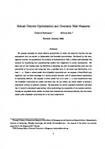
Figure 5. Convergence history of minimum weight for 25-bar space truss (Example 1) Figure 5 shows a comparison of the convergence capability of each HS case and the GAbased approaches. While the pure GA proposed by Rajeev and Krishnamoorthy [10] obtained a minimum weight of 546.01 lb after 600 structural analyses, the HS cases obtained minimum weights of 504.28 to 521.04 lb after the same number of analyses. The steady-


117

state GA proposed by Wu and Chow [13] obtained a minimum weight of 486.29 lb after 40,000 analyses, while all HS cases except Case 1 obtained the same weight after 2,160 to 6,850 analyses. These results suggest that the HS-based method is a powerful search and discrete size optimization technique, as compared to pure and steady-state GA-based methods, in terms of both the obtained optimal value and the convergence capability. Example 2: 72-bar space truss The 72-bar space truss, shown in Figure 6, is one of the most popular classical optimization design problems, and has been used as a benchmark to verify the efficiency of various optimization methods. The majority of these studies have assumed that the cross-sectional areas (size variables) were continuous. However, Wu and Chow [13] optimized this space structure with discrete cross-sectional areas using the steady-state GA-based method. In this example, the material density and modulus of elasticity were 0.1 lb/in.3 and 10,000 ksi, respectively. The space truss was subjected to the following two loading conditions: Condition 1, in which PX = 5.0 kips, PY = 5.0 kips, and PZ = -5.0 kips on node 17; and Condition 2, in which PX = 0.0 kips, PY = 0.0 kips, and PZ = -5.0 kips on nodes 17, 18, 19, and 20. The structure was required to be doubly symmetric about the X- and Y-axes. This condition divided the truss members into the following sixteen groups: (1) A1 ~ A4, (2) A5 ~ A12, (3) A13 ~ A16, (4) A17 ~ A18, (5) A19 ~ A22, (6) A23 ~ A30, (7) A31 ~ A34, (8) A35 ~ A36, (9) A37 ~ A40, (10) A41 ~ A48, (11) A49 ~ A52, (12) A53 ~ A54, (13) A55 ~ A58, (14) A59 ~ A66, (15) A67 ~ A70, and (16) A71 ~ A72. The members were subjected to stress limitations of  25 ksi, and the maximum displacement of the uppermost nodes was not allowed to exceed  0.25 in. for each node, in all directions. In this example, the available discrete values for the cross-sectional areas were chosen from the sixty-four discrete values listed in Table 3. Table 3. Available discrete cross-sections No. (1) Areas (2) No. (3) 1 0.111 17 2 0.141 18 3 0.196 19 4 0.250 20 5 0.307 21 6 0.391 22 7 0.442 23 8 0.563 24 9 0.602 25 10 0.766 26 11 0.785 27 12 0.994 28 13 1.000 29 14 1.228 30 15 1.266 31 16 1.457 32 Note: cross-sectional areas are in in.2.

Areas (4) 1.563 1.620 1.800 1.990 2.130 2.380 2.620 2.630 2.880 2.930 3.090 3.130 3.380 3.470 3.550 3.630

No. (5) 33 34 35 36 37 38 39 40 41 42 43 44 45 46 47 48

Areas (6) 3.840 3.870 3.880 4.180 4.220 4.490 4.590 4.800 4.970 5.120 5.740 7.220 7.970 8.530 9.300 10.850

No. (7) 49 50 51 52 53 54 55 56 57 58 59 60 61 62 63 64

Areas (8) 11.500 13.500 13.900 14.200 15.500 16.000 16.900 18.800 19.900 22.000 22.900 24.500 26.500 28.000 30.000 33.500

118

KANG SEOK LEE, SANG WHAN HAN, and ZONG WOO GEEM Y 120 in.

Typical Story (8)

120 in.

9 4

16

X Z

12 (4) 13

(5)

(17)

(18)

1

17

11 5

6

15 10

(7) 3

18 14 8

(6)

(3)

7

2

60 in. (1) (13)

(14)

(9)

(10)

(2)

Element and node numbering system of the typical story

//

240 in. //

(6) (5)

60 in. (1)

X

(2)

Figure 6. 72-Bar Space Truss Table 4. Optimal results for 72-bar space truss (Example 2) HS results Design variables Ai (in.2) (1)

Case-1 (2)

Case-2 (3)

Case-3 (4)

Wu and Chow (1995b) Case-4 (5)

Case-5 (6)

b

1X (7)

b

2X (8)

b

3X (9)

b

4X (10)

Xicheng & Guixu (1992)c (11) 1.905 0.518 0.100 0.100 1.286 0.516 0.100 0.100 0.509 0.522 0.100 0.100 0.157 0.537 0.411 0.571 380.84

Erbatur et al. (2000)c (12)

1.910 1.563 1.990 1.990 1.563 1.620 1.990 1.990 A1 ~ A4 1.990 1 1.800 0.525 0.766 0.563 0.602 0.307 0.602 0.602 0.442 0.602 2 A5 ~ A12 0.602 0.122 0.141 0.111 0.141 0.111 0.111 0.111 0.111 0.111 3 A13 ~ A16 0.111 0.103 0.111 0.141 0.111 0.111 0.111 0.111 0.111 0.111 4 A17 ~ A18 0.111 1.310 1.800 1.457 0.994 2.130 1.457 1.457 1.266 1.228 5 1.457 A19 ~ A22 0.498 0.602 0.602 0.602 0.602 0.391 0.391 0.563 0.563 6 0.563 A23 ~ A30 0.110 0.141 0.111 0.111 0.111 0.111 0.141 0.111 0.111 7 0.111 A31 ~ A34 0.103 0.307 0.111 0.307 0.111 0.111 0.111 0.111 0.111 8 0.111 A35 ~ A36 0.535 0.391 0.442 0.307 0.766 0.563 0.391 0.391 0.442 9 0.442 A37 ~ A40 0.535 0.391 0.766 0.602 1.000 0.563 0.602 0.602 0.442 10 A41 ~ A48 0.442 0.103 0.141 0.111 0.111 0.111 0.111 0.111 0.111 0.111 11 A49 ~ A52 0.111 0.111 0.111 0.141 0.563 0.111 0.111 0.111 0.111 0.111 12 A53 ~ A54 0.141 0.161 0.196 0.196 0.250 0.785 0.196 0.196 0.196 0.196 13 A55 ~ A58 0.196 0.544 0.602 0.442 0.766 0.602 0.602 0.602 0.563 0.563 14 A59 ~ A66 0.563 0.379 0.307 0.250 0.307 0.602 0.391 0.391 0.391 0.391 15 A67 ~ A70 0.250 0.521 0.766 1.000 0.391 0.602 0.785 0.563 0.563 0.563 16 A71 ~ A72 1.000 Weight (lb) 400.63 390.62 390.30 399.23 396.38 471.98 439.77 428.00 427.20 383.12 Number of 25,717 26,812 21,901 13,866 22,894 60,000 60,000 60,000 60,000 structural [7,242]a [7,462]a [3,711]a [4,819]a [3,677]a analyses a Number of analyses for the HS required to obtain a weight of 427.2 lb (the best result of Wu and Chow, 1995b). b Crossover operators used by Wu and Chow (1995b). c The optimal results of continuous size optimization.


119

Figure 7 shows a comparison of the convergence capability of each HS case and the steady-state GA-based method [13]. Wu and Chow obtained a minimum weight of 427.2 lb after 60,000 structural analyses using a four-point crossover operator, while the proposed HS approach obtained the same weight after 3,711 to 7,462 analyses. The HS approach therefore outperformed the steady-state GA-based method, in terms of both the obtained optimal value and the convergence capability. The best HS optimum solution (Case-3, 21901 searches, 390.3 lb)

4000

Note: * denotes a weight calculated by the best solution vector from harmony memory

3500

Case-1 Case-2 Case-3 Case-4 Case-5

3000

*

Weight (lb)

2500 2000

Number of analyses for HS required to obtain a weight of 427.20 lb (A)

1500 1000

GA Optimal solution A:Wu and Chow (1995b)

500

A(60000, 427.20 lb)

0 1

10

100

1000

10000

Number of searches (FEM analyses)

Figure 7. Convergence history of minimum weight for 72-bar space truss (Example 2)

6. DISCRETE-CONTINUOUS CONFIGURATION OPTIMIZATION EXAMPLES Example 3: 25-bar space truss The 25-bar transmission tower space truss shown in Figure 4, which was previously studied by Wu and Chow [9] using the GA-based method, was also analyzed to optimize both the sizes of the discrete members and the continuous geometric variables. The design details, such as the material properties, constraints, loading condition, truss member groups, and set of available discrete cross sections, were the same as those used in Example 1. For the configuration optimization, the geometric variables of the structure were selected as coordinates X4, Y4, Z4, X8, and Y8, with symmetry required in X-Z and Y-Z planes. Hence, there were thirteen independent design variables, including the eight sizing variables given in Example 1 and five geometric variables. The side constraints for the geometric variables, i.e., the lower and upper bounds on the nodal coordinates, were 20  X4  60, 40  Y4  80, 90  Z4  130, 40  X8  80, and 100  Y8  140 (in.).


120

The HS-based discrete-continuous configuration optimization method was applied to the 25-bar space truss using each set of parameters shown in Table 1. The algorithm found the best solution vector (i.e., the values of the eight sizing variables and five geometric variables) with each set of parameters within 30,000 searches. Table 5 gives the best solution and the corresponding minimum structural weight for each case, and also provides a comparison between the optimal design result reported by Wu and Chow [9] and the present work. The best minimum weight of 123.77 lb was obtained using the Case 5 parameters after 8,902 searches (structural analyses), and this minimum weight converged remarkably after only 2,000 searches. The results from each HS case were better than the previous design result reported by Wu and Chow [9], and the HS best result using the Case 5 parameters produced a weight saving of 10%, as compared to the GA-based method proposed by Wu and Chow [9]. The configuration optimization achieved an amazing optimal weight saving of 70%, as compared to the pure HS size optimization, which obtained a best minimum weight of only 484.85 lb, as shown in Table 2. Table 5. Optimal results of 25-bar space truss (Example 3) Design variables Ai (in.2) & Ri (in.)

Case-2

Case-3

Case-4

Case-5

(1995a)

(2)

(3)

(4)

(5)

(6)

(7)

1

A1

0.1

0.1

0.1

0.2

0.2

0.1

2

A2 ~ A5

0.2

0.1

0.2

0.2

0.1

0.2

3

A6 ~ A9

0.9

1.0

0.9

1.0

0.9

1.1

4

A10 ~ A11

0.1

0.1

0.1

0.1

0.1

0.2

5

A12 ~ A13

0.1

0.1

0.1

0.2

0.1

0.3

6

A14 ~ A17

0.1

0.1

0.2

0.1

0.1

0.1

7

A18 ~ A21

0.1

0.4

0.2

0.1

0.2

0.2

8

A22 ~ A25

1.2

0.7

0.8

1.0

1.0

0.9 41.07

(1)

1

X4

31.64

28.54

29.51

27.94

31.88

2

Y4

66.30

55.18

56.76

55.21

53.57

53.47

3

Z4

102.22

127.80

130.0

123.70

126.35

124.60

4

X8

40.00

43.02

40.43

50.80

Y8

125.74

136.66

41.74 133.62

43.63

5

130.83

130.64

131.48

129.34

123.81 a

[138.10] Weight (lb)

[130.40]

b c

Number of structural analyses a

Wu & Chow

HS results Case-1

126.07 a

[152.10]

b

[140.63]

c

126.74

[154.05] [141.65]

a

b c

123.77 a

[137.79]a

b

[124.28]b

c

[123.86]c

[168.09] [146.68]

[129.53]

[134.29]

[131.71]

[133.87]

[129.36]d

[124.92]d

[131.03]d

[128.16]d

[123.80]d

29,290

9,646

23,100

19,833

8,902

136.20

-

The structural weights obtained after 1,000 analyses. b The structural weights obtained after 2,000 analyses. c The structural weights obtained after 3,000 analyses. d The structural weights obtained after 8,000 analyses.


121

Example 4: 47-bar planar power line tower The 47-bar planar power line tower design, shown in Figure 8, was the last example used to demonstrate the practical capability of the HS algorithm-based structural optimization method. This tower was previously analyzed by Felix [26] and Hansen and Vanderplaats [27] to obtain optimal continuous size and geometric variables (i.e., a continuous configuration optimization). In this problem, the structure had forty-seven members and twenty-two nodes, and was symmetric about the Y-axis. All members were made of steel, and the material density and modulus of elasticity were 0.3 lb/in.3 and 30,000 ksi, respectively. This tower was designed for three separate load conditions: (1) 6.0 kips acting in the positive X-direction and 14.0 kips acting in the negative Y-direction at nodes 17 and 22, (2) 6.0 kips acting in the positive X-direction and 14.0 kips acting in the negative Y-direction at node 17, and (3) 6.0 kips acting in the positive X-direction and 14.0 kips acting in the negative Y-direction at node 22. The first condition represented the load imposed by two power lines attached to the tower at an angle. The second and third conditions represented cases that occur when one of the two lines snaps. 150 in. 90 in. 30 in. (17)

23 (18) 25 (19) 27 (20) 26 (21) 21

19

20

17

13 15

24

(22)

600 in.

22

16 14

18

(15)

(16) 11 (13) 2

10 9

(14)

12

7

(12)

540 in.

4

8

(11)

480 in.

6 1

29

3

5 28

(9) 31

32 33

(7)

420 in.

(10) 30 (8)

360 in.

37 34

35 36 38

(5)

(6)

240 in.

42 39

40 41 43

(3)

(4)

120 in.

47 44

45 46

Y (1)

X 60 in.

(2)

60 in.

Figure 8. 47-bar planar power line tower

0

122


The structure was subjected to both stress and buckling constraints. The stress constraints were 15.0 ksi in compression and 20.0 ksi in tension. The Euler buckling compressive stress limit for each member i was used for the buckling constraints. This was computed as  icr 

 KEAi (i  1,...,47) L2i

(7)

where K is a constant determined from the cross-sectional geometry, E is the modulus of elasticity of the material, and Li is the member length. In this study, the buckling constant was K = 3.96. The cross-sectional areas of the members were categorized into twenty-seven groups, as follows: (1) A1 = A3, (2) A2 = A4, (3) A5 = A6, (4) A7, (5) A8 = A9, (6) A10, (7) A11 = A12, (8) A13 = A14, (9) A15 = A16, (10) A17 = A18, (11) A19 = A20, (12) A21 = A22, (13) A23 = A24, (14) A25 = A26, (15) A27, (16) A28, (17) A29 = A30, (18) A31 = A32, (19) A33, (20) A34 = A35, (21) A36 = A37, (22) A38, (23) A39 = A40, (24) A41 = A42, (25) A43 , (26) A44 = A45, and (27) A46 = A47. The independent geometric variables were X2, X4, Y4, X6, Y6, X8, Y8, X10, Y10, X12, Y12, X14, Y14, X20, Y20, X21, and Y21. The geometric variables were linked to maintain symmetry about the Y-axis. Nodes 1 and 2 were required to remain at Y = 0.0, and the coordinates of nodes 15, 16, 17, and 22 were not changed. There were forty-four independent design variables, including twenty-seven sizing variables and seventeen coordinate variables. In this example, the cross-sectional areas were chosen from the sixty-four discrete values listed in Table 3, and a pure discrete sizing variable problem (with fixed geometry) was also optimized for comparison. Table 6 gives the optimal results obtained using each set of HS parameters for the discrete-continuous configuration optimization, along with the optimal results for the continuous configuration problem. The best pure discrete size result, which was obtained using the Case 3 parameters, is also listed in the table. After 73,257 to 76,937 searches (structural analyses), the best discrete-continuous solution vector and the corresponding objective function value were obtained for each HS case. The best minimum weight of 2,020.78 lb was obtained using the Case 1 parameters after 73,771 searches, and this minimum weight converged remarkably after 40,000 searches. The discrete-continuous configuration optimization produced a considerable weight saving of 16%, as compared to the pure discrete size optimization, which obtained a minimum weight of 2,396.8 lb.


123

Table 6. Optimal results of 47-bar planar power line Design variables Ai (in.2) & Ri (in.) (1) 1 2 3 4 5 6 7 8 9 10 11 12 13 14 15 16 17 18 19 20 21 22 23 24 25 26 27 1 2 3 4 5 6 7 8 9 10 11 12 13 14 15 16 17

A1 = A3 A2 = A4 A5 = A6 A7 A8 = A9 A10 A11 = A12 A13 = A14 A15 = A16 A17 = A18 A19 = A20 A21 = A22 A23 = A24 A25 = A26 A27 A28 A29 = A30 A31 = A32 A33 A34 = A35 A36 = A37 A38 A39 = A40 A41 = A42 A43 A44 = A45 A46 = A47 -X1=X2 -X3= X4 Y3=Y4 -X5=X6 Y5=Y6 -X7=X8 Y7=Y8 -X9=X10 Y9=Y10 -X11=X12 Y11=Y12 -X13=X14 Y13=Y14 -X18=X21 Y18=Y21 -X19=X20 Y19=Y20

Weight (lb)

HS results Pure Size Case-3* (2) 3.840 3.380 0.766 0.141 0.785 1.990 2.130 1.228 1.563 2.130 0.111 0.111 1.800 1.800 1.457 0.442 3.630 1.457 0.391 3.090 1.457 0.196 3.840 1.563 0.196 4.590 1.457 60.0* 60.0* 120.0* 60.0* 240.0* 60.0* 360.0* 30.0* 420.0* 30.0* 480.0* 30.0* 540.0* 90.0* 600.0* 30.0* 600.0* 2,396.8 [2,471.1]a [2,434.3]b [2,407.7]c

Case-1 (3)

Case-2 (4)

Case-3 (5)

Case-4 (6)

Case-5 (7)

2.620 2.630 1.228 0.196 1.000 1.620 1.800 0.785 1.000 1.563 0.391 0.766 1.228 1.228 1.228 0.196 2.930 0.994 0.111 3.470 1.000 0.111 3.380 1.228 0.111 3.380 0.994 98.9 80.9 114.8 62.8 236.9 51.3 315.9 47.9 387.4 50.3 477.3 41.4 521.4 92.5 615.3 14.3 596.5 2,020.78 [2,428.62]a [2,198.13]b [2,066.73]c

3.550 3.090 0.766 0.141 1.000 1.228 1.990 1.000 1.228 1.800 0.602 0.994 1.457 1.457 1.228 0.250 2.880 1.228 0.111 2.880 1.000 0.111 3.130 1.266 0.111 3.470 1.563 89.4 83.1 111.7 74.4 234.9 59.5 339.3 40.7 429.6 35.2 455.3 34.4 505.7 83.9 609.2 18.4 586.4 2,116.14 [2,608.26]a [2,339.84]b [2,195.27]c

3.130 3.090 1.000 0.111 0.994 1.228 2.130 0.785 1.228 1.990 0.785 0.994 1.457 1.457 1.000 0.111 2.880 0.994 0.141 3.130 1.228 0.307 3.380 1.000 0.111 3.630 1.266 85.9 80.9 115.4 61.6 233.9 55.4 319.4 46.9 409.9 35.3 471.8 36.6 504.9 84.8 606.8 17.1 582.0 2,091.21 [2,580.55]a [2,361.17]b [2,189.57]c

3.090 2.880 0.994 0.141 1.228 1.620 2.380 0.602 1.228 1.620 0.563 1.457 1.228 1.228 1.457 0.141 3.130 0.994 0.111 3.380 1.000 0.111 3.470 1.228 0.250 3.470 0.994 97.7 80.9 114.1 60.1 225.2 49.2 323.1 44.4 392.1 38.1 477.3 40.1 519.2 91.3 620.9 6.9 580.7 2,096.35 [2,735.43]a [2,421.92]b [2,225.39]c

2.930 2.630 1.228 0.141 0.994 1.800 2.380 0.602 0.994 1.620 0.602 1.228 1.228 1.228 1.457 0.196 3.130 0.766 0.111 3.550 1.000 0.111 3.380 1.000 0.111 3.470 1.266 91.6 80.9 122.9 61.6 238.4 47.6 327.9 41.1 394.1 42.7 476.6 42.4 504.7 84.7 615.5 3.2 569.6 2,056.77 [2,468.82]a [2,269.06]b [2,165.42]c

Number of 45,557 73,771 76,937 74,721 76,828 73,257 analyses * ** Coordinate is stationary. The results of continuous configuration optimizations. a Structural weights obtained after 10,000 analyses. b Structural weights obtained after 20,000 analyses. c Structural weights obtained after 40,000 analyses.

Felix** (1981) (8)

Hansen & Vanderplaats**(1990) (9)

2.73 2.47 0.73 0.21 0.94 1.08 1.69 0.69 1.06 1.41 0.26 0.81 1.06 1.05 0.82 0.30 2.77 0.66 0.21 2.90 0.27 1.41 3.43 0.99 0.17 3.65 1.01 90.0 90.0 123.4 83.4 244.5 70.5 355.1 60.0 425.0 58.2 478.0 59.6 519.5 96.9 633.7 15.0 607.6

2.42 2.35 0.82 0.10 0.86 1.15 1.77 0.67 0.86 1.24 0.33 1.22 0.93 0.86 0.69 0.15 2.46 0.90 0.10 2.74 0.92 0.10 2.94 1.13 0.10 3.12 1.10 107.1 91.2 122.8 74.2 241.4 65.5 324.6 57.1 400.4 49.3 472.3 47.4 507.5 83.3 636.0 3.9 586.5

1,904.0

1,850.4

-

-

124


7. CONCLUSIONS Pure discrete size and integrated discrete size and continuous configuration optimization methods for structural systems, based on the HS algorithm, were proposed in this paper. Several standard truss examples from the literature were also presented to demonstrate the effectiveness and robustness of the proposed method. The results were compared to those obtained using current discrete optimization methods, especially GA-based techniques. The illustrative examples revealed that the HS optimal results were better than those obtained from all previous investigations. Also, the convergence capability of the proposed HS approach outperformed that of the GA-based methods. Therefore, our study suggests that the new HS-based method is a potential powerful search and optimization technique for solving structural optimization problems with discrete sizing variables. The recently developed HS heuristic algorithm is simple and mathematically less complex than the GA. The HS algorithm generates new vectors, based on the harmony memory considering rate and the pitch adjusting rate, after considering all of the existing vectors, while the GA generates a new vector from only two of the existing vectors (parents). These features increase the flexibility of the HS algorithm and allow it to find better solutions. Furthermore, the HS algorithm adopted a parameter-setting-free adaptive feature, enabling the algorithm users not to perform tedious parameter setting process [28, 29]. The HS algorithm-based method proposed in this study is not limited to truss structural optimization problems. Besides trusses, the HS algorithm can also be applied to other types of structural optimization problems, including frame structures, plates, and shells.

Acknowledgments: This study was carried out with financial support from the Korea Research Foundation Grant founded by the Korean Government (MOEST) (The Regional Research Universities Program/Biohousing Research Institute) and the Seoul R&BD Program (PA100071).

REFERENCES 1. 2. 3. 4.

5.

6.

Lipson L, Gwin LB. Discrete sizing of trusses for optimal geometry, J Struct Div ASCE 1977; 103(ST5): 1031-46. Liebman JS, Khachaturian N, Chanaratna V. Discrete structural optimization, J Struct Div ASCE 1981; 107(ST11): 2177-97. Hua HM. Optimization for structures of discrete-size elements, Comput Struct 1983; 17(3): 327-33. Templeman AB, Yates DF. Nonlinear programming approach to discrete optimum design of trusses, Optimization methods in structural design. Eschenauer H., Olhoff N., eds., BI Wissenschaftsverlag, Mannheim, Germany, 1983. John KV, Ramakrishnan CV. Minimum weight design of trusses using improved move limit method of sequential linear programming, Comput Struct 1987; 27(5): 583-91. Templeman AB. Discrete optimum structural design, Comput Struct 1988; 30(3): 511-8.


7.

8. 9. 10. 11. 12. 13. 14. 15. 16. 17. 18. 19. 20.

21. 22. 23. 24. 25. 26. 27.

125

Bremicker M, Papalambros PY, Loh HT. Solution of mixed-discrete structural optimization problems with a new sequential linearization algorithm, Comput Struct 1990; 37(4): 451-61. Zhu DE. An improved templeman’s algorithm for optimum design of trusses with discrete member sizes, Eng Optimiz 1993; 9: 303-12. Wu S-J, Chow P-T. Integrated discrete and configuration optimization of trusses using genetic algorithms, Comput Struct 1995; 55(4): 695-702. Rajeev S, Krishnamoorthy CS. Discrete optimization of structures using genetic algorithms, J Struct Eng ASCE 1992; 118(5): 1233-50. Rajeev S, Krishnamoorthy CS. Genetic algorithm-based methodologies for design optimization of trusses. J Struct Eng ASCE 1997; 123(3): 350-8. Lin CY, Hajela P. Genetic algorithms in optimization problems with discrete and integer design variables, Eng Optimiz 1992; 19(4): 309-27. Wu S-J, Chow P-T. Steady-state genetic algorithms for discrete optimization of trusses, Comput Struct 1995; 56(6): 979-91. Camp C, Pezeshk S, Cao G. Optimized design of two-dimensional structures using a genetic algorithm, J Struct Eng ASCE 1998;124(5): 551-9. Pezeshk S, Camp CV, Chen D. Design of nonlinear framed structures using genetic optimization, J Struct Eng ASCE 2000: 126(3): 382-8. Erbatur F, Hasancebi O, Tutuncil I, Kihc H. Optimal design of planar and space structures with genetic algorithms. Comput Struct 2000; 75: 209-24. Holland JH. Adaptation in natural and artificial systems, University of Michigan Press, Ann Arbor, MI, 1975. Goldberg DE. Genetic algorithm in search optimization and machine learning. Addision Wesley, Boston, MA, 1989. Lee KS, Geem ZW. A new structural optimization method base on harmony search algorithm, Comput Struct 2004; 82: 781-98. Lee KS, Geem ZW. A new meta-heuristic algorithm for continuous engineering optimization: harmony search theory and practice, Comput Method Appl M 2005; 194: 3902-33. Geem, ZW, Kim J-H, Loganathan GV. A new heuristic optimization algorithm: harmony search, Simulation 2001; 76(2): 60-8. Geem ZW. Novel Derivative of Harmony Search Algorithm for Discrete Design Variables, Appl Math Comput 2008; 199(1): 223-30. Geem ZW. Optimal Cost Design of Water Distribution Networks Using Harmony Search, Eng Optimiz 2006; 38(3): 259-80. Adeli H, Park HS. Hybrid CPN-neural dynamics model for discrete optimization of steel structures, Microcomput Civil Eng 1996; 11(5): 355-66. Park HS, Sung CW. Optimization of steel structures using distributed simulated annealing algorithm on a cluster of personal computers, Comp Struct 2002; 80: 1305-16. Felix JE. Shape optimization of trusses subjected to strength, displacement, and frequency constraints, Masters Thesis, Naval Postgraduate School, 1981. Hansen SR, Vanderplaats GN. Approximation method for configuration optimization of trusses, AIAA J 1990; 28(1): 161-68.

126

28. 29. 30.


Xicheng W, Guixu M. A parallel iterative algorithm for structural optimization, Comput Method Appl M 1992; 96: 25-32. Geem ZW, Sim K-B. Parameter-Setting-Free Harmony Search Algorithm, Appl Math Comput 2010; 217(8): 3881-9. Hasancebi O, Erdal F, Saka MP. Adaptive Harmony Search Method for Structural Optimization, J Struct Eng ASCE 2010; 136(4): 419-31.