discrete stochastic optimization using linear interpolation

Proceedings of the 2008 Winter Simulation Conference S. J. Mason, R. R. Hill, L. Mönch, O. Rose, T. Jefferson, J. W. Fowler eds.

DISCRETE STOCHASTIC OPTIMIZATION USING LINEAR INTERPOLATION

Honggang Wang Bruce W. Schmeiser School of Industrial Engineering Purdue University West Lafayette, IN 47907, U.S.A.

tor defined on some probability space, such that Y (x) = ∑ki=1 Y (x, ωi )/k → g(x) almost surely, as k → ∞, ∀ x ∈ X.

ABSTRACT We consider discrete stochastic optimization problems where the objective function can only be estimated by a simulation oracle; the oracle is defined only at the discrete points. We propose a method using continuous search with simplex interpolation to solve a wide class of problems. A retrospective framework provides a sequence of deterministic approximating problems that can be solved using continuous optimization techniques that guarantee desirable convergence properties. Numerical experiments show that our method finds the optimal solutions for discrete stochastic optimization problems orders of magnitude faster than existing random search algorithms. 1

Assumption 3. There exists an optimum set M∗ , such that M∗ 6= 0/ and ∀x∗ ∈ M∗ , g(x∗ ) is finite. We also need following defintions to define our problem statement. Definition 1. The local neighborhood of an integer point x ∈ X is N(x) = {x0 : x0 ∈ X, ||x0 − x|| ≤ 1}, where X is the feasible set of function g and ||x|| is the Euclidean norm of vector x. Definition 2. x∗ ∈ X is called a local optimizer of a function g in a feasible region X, if g(x0 ) ≤ g(x) ∀x0 ∈ N(x∗ ) ∩ X.

INTRODUCTION

Definition 3. The optimal set M∗ of a function g is the set of all local optimizers of g over the feasible set X.

Many methods have been developed to solve discrete stochastic optimization (DSO) problems as discussed in (Andrad´ottir 1998, Fu et al. 2005, Swisher et al. 2000). Most of the approaches for large-size DSO problems seek to find the optimum through the discrete space using random search.

We want to design algorithms to find one of the local optimizers x∗ in the optimal set M∗ of objective function g over set X, given a simulation oracle Y (x, ω) provided that the sample mean of Y (x) consistently estimates g(x) for all x ∈ X. Thus, we define our problem statement in a stochastic form of IP: (ISP) find an x∗ that minimizes g locally, provided that a simuluation oracle Y consistently estimates g.

1.1 Problem Statement We consider discrete optimization problems of the form (IP) find x∗ such that x∗ ∈ argmin g(x) x∈X

1.2 Background and Motivation

where g is a real-valued function on X, X ⊆ Zd and Zd is the set of d-dimensional integer vectors. The discrete DSO problems of interest have the form of IP with the following three assumptions:

In many practical applications of stochastic optimization, the objective function is usually estimated by an expensive simulation process and the problem IP itself is NP-hard. For instance, consider a classical (s, S) inventory problem (Pichitlamken and Nelson 2003, Koenig and Law 1985), where s is the reorder point and S is the order-up-to level. Assume that the level of inventory of units is periodically reviewed, we want to find the inventory levels of units

Assumption 1. The function g is bounded on any closed subset of X. Assumption 2. There is a simulation oracle that returns Y (x, ω), for every x ∈ X and the ω is the random vec-

978-1-4244-2708-6/08/$25.00 ©2008 IEEE

502

Wang and Schmeiser of products for a manufacturing plant such that it yields the maximum expected profits. If the production times are truncated normal distributions and the demand times and quantities are distributed exponentially and uniformly respectively, then the problem cannot be solved analytically. The objective function is not available analytically but can be evaluated with noise by simulating the stochastic system. The simulation evaluation, however, is computationally expensive and returns only the estimates of the function with limited sample size. One wants to limit the number of function evaluations while get the function estimates at a high-level accuracy. A continuous search can save computing iterations with the guided improving directions. Can we search the discrete space “continuously” by creating gradient-type directions?

more-reliable continuous search methods to solve discrete optimization problems. We want to define, for instance, what x = {4.6, 2.3, 0.8} means in an integer parameter setting problem. How can 4.6 machines be simulated in the simulation model? Some type of continuous interpolation is required on the integral points. Coupling with data interpolation, we create a continuous function f : Q → R, Q ⊆ Rd T and Q Zd = X, such that f (z) = g(z), ∀ z ∈ X. The original integer problem is relaxed in the sense that the domain of the objective function of IP is now a connected subset Q in Euclidean space Rd . This relaxation is different from the usual continuous relaxation, since except the grid integral points all the continuous points do not have any real values and physical meanings in our problems. The function values are created at fractional points only for the purpose of continuous search.

1.3 Proposed Method 2.2 Multiple-Dimensional Continuous Interpolation We propose a continuous search method with linear interpolation for DSO problems. Instead of random search, we search the optimal solutions through a constructed continuous space. Piecewise-linear interpolation creates a continuous response surface that agrees with g at all feasible points in X. We use retrospective optimization approach to solve the constructed continuous stochastic problem with nonlinear derterministic optimization tools. Kriging (Biles et al. 2007, Huang et al. 2006) is another approach to stochastic optimization via simulation that relies on interpolation of the response surface. 2

In multiple-dimensional Euclidean space, interpolating data on grid points is an easy way to create a continuous function with desirable features through the whole space. Data interpolation provides a continuous function that agrees with true function values g at every integral point x ∈ X. The extreme points in the domain of the interpolated function are always integral point in X. We can use multi-linear interpolation (Weiser and Zarantonello 1988) on the entire unit cube, however, the dimensionality issue implies that d-cube interpolation may consume a lot of computing resource, as the number of vertices of a unit hyper-cube is 2d . A simplex interpolation is a faster alternative, because it requires only d + 1 vertices for calculating the function value at any point x in that simplex.

CONSTRUCTION OF CONTINUOUS RESPONSE USING LINEAR INTERPOLATION

A continuous response surface that connects all integer response points of ISP reveals the curvature information of its objective function g. This curvature of g often helps search algorithms mover faster toward the optimum of g. Simplex interpolation creates piecewise-linear continuous surface fast and offers nice properties.

2.3 Simplex Piecewise-Linear Interpolation We use the method described in (Weiser and Zarantonello 1988) and (Rovatti et al. 1998) to interpolate the integer-ordered data on every feasible simplex defined by integer vertices in X. The interpolation partitions the real set Q to a collection of closed simplices {Si }i∈K , where Si denotes a unit simplex defined by neighboring integer points in X. We define the simplex-interpolation routine as follows.

2.1 Continuous Relaxation To do continuous search in the solution space we create a continuous response surface for the discrete problem IP. Nonetheless the objective function in IP or in ISP is often defined at x ∈ X in the discrete space. Doing continuous relaxation by dropping the integral constraints on these variables is typically not applicable because a fractional number of machines or workers does not make any sense in real world. A half of machine or 1.4 workers or machines are not defined in our simulation model. Although the function g is not defined at non-integer points, we like to be able to search on these fractional points, since that provides us the possibility using the faster and

Routine SI Given: A point x ∈ Q and a function g on X; Return: f (x). (i) (ii) (iii)

503

Locate the unit cube containing x by identifying the “lower left” vertex of the cube, which is bxc; Let x0 = x − bxc, a point in the unit cube; Sort the components of x0 to obtain x0p(1) ≥ x0p(2) ≥ . . . ≥ x0p(d) . As a permutation of {1, . . . , d}, {p(1), p(2), . . . , p(d)} defines a simplex enclosing

Wang and Schmeiser

(iv)

x with the vertices x0 , x1 , . . . , xd , where x0 = bxc, xi = xi−1 + ei , and ei is the unit vector with the p(i)th element equal to 1, for i = 1, 2, . . . , d; construct the function f using

3

With the construction of continuous response surface using simplex interpolation, we create a class of continuous stochastic optimization (CSO) problems of the form CSP. The objective functions of these CSO problems are continuous and piecewise linear on their domains. The classical Stochastic Approximation (Kushner and Clark 1978) approach cannot be applied to these CSO problems due to the nondifferentiability of objective functions at the boundary points. Although CSO problems generally are not continuously differentiable, the piecewise linearity makes them tractable due to the developed theories of nondifferentiable analysis. In particular if CSO is convex, there are many convex optimization tools adaptable for stochastic settings, e.g. stochastic subgradient methods (Shor 1985) and conjugate gradient search (Hiriart-Urruty and Lemarechal 1993). The Retrospective Optimization (RO, also called sample average approximation method) approach offers us a general setting in that we can use deterministic nonlinear optimization tools for solving a convergent sequence of approximating problems of CSP. The sequence of the sample path problems converges to CSP w.p.1 as the sample size goes to infinity under the Assumption 2.

d

  0 p(i) 0 p(i+1) f (x) = ∑ g(xi )(x −x ) ,

(1)

i=0

where x0p(0) = 1 and x0p(d+1) = 0. For a fixed simplex, the integral components bxc of a design point x are constant integers; thus Equation 1 is a linear function of x. Replacing the deterministic function values g(xi ) in (1) with the stochastic simulation oracle Y (xi , ω), for i = 0, 1, . . . , d, we obtain the stochastic form to estimate the function value f (x) at any point x ∈ Q. We extend Y (x) to the real set Q based on simplex-interpolation routine SI d

  0p(i) 0p(i+1) −x ) . Y (x, ω) = ∑ Y (xi , ω)(x

RETROSPECTIVE OPTIMIZATION FRAMEWORK FOR STOCHASTIC PIECEWISELINEAR OPTIMIZATION PROBLEMS

(2)

i=0

From Assumption 2, Equation (2) allows the consistent estimation of f (x) at any x ∈ Q using the sample average Y k (x). 2.4 Constructed Continuous Response Surface

3.1 The Sample-Path Approximation Approach

We present some of the properties of simplex interpolation discussed in (Weiser and Zarantonello 1988) without proofs.

Healy and Schruben (1991) propose the retrospective approach for stochastic optimization. The fundamental idea of the RO algorithms is simple. It generates a sample of the random inputs and uses the sample average of system observations to approximate f in CSP. With a fixed sample of random vectors, CSP becomes deterministic. One can solve the approximating problem with deterministic optimization tools. As discussed in (Spall 2005), retrospective optimization approach has some noticeable advantages: (a) there are many powerful deterministic search methods applicable and robust optimization tools for handling complex constraints; (b) for a fixed sample path, it is possible to conduct a large number of iterations of deterministic search at nominal cost. Chen and Schmeiser (1994) propose the retrospective approximation in the context of stochastic root finding. Instead of solving one sample-path problem, they generate and solve a sequence of sample-path problems {Pk } with increasing sample sizes {mk } and decreasing sequence of tolerance errors. Jin and Schmeiser (2003) develop a retrospective optimization algorithm to solve continuous stochastic optimization problems with general constraints. Shapiro and Wardi (1996) analyze the convergence properties of a gradient-based implementation of RO method. Kleywegt et al. (2001) use the RO approach to solving a

Proposition 1. f (x) = g(x), ∀x ∈ X. Proposition 2. The constructed function f is continuous and piecewise linear on its domain Q. Proposition 3. Given a point x in Rd , the simplex enclosing x created by the interpolation is uniquely identified. Proposition 4. The set of created simplices is a partition of the domain Q of f . The simplex-interpolation also provides following proposition: Proposition 5. An integer optimum of g is also an optimal point of f . With these properties provided by the simplex interpolation, the ISP problem is converted to a continunous stochastic optimization (CSO) problem with desirable characteristics: (CSP) Find a local optimizer x∗ of function f over the feasible set Q, where f can be consistently estimated by the simulation oracle Y (x, ω), where ω is the random effects in the simulation model, Q ⊆ R, and Q ∩ Zd = X.

504

Wang and Schmeiser the increasing sample sizes {mk }; a strategy for sampling ξk = {ω 1 , . . . , ω mk } across iterations; calculation of a starting solution for each Pk ; determining a decreasing sequence of error tolerance {εk } for sample path problems {Pk }. In addition, a deterministic method must be chosen to solve each sample path problem Pk before we develop an efficient retrospective optimization method. Seeking an exact solution for each Pk is time consuming and not necessary since Pk itself is an approximating problem of true problem CSP. Thus approximated εk -solutions for those sample path problems are desirable.

stochastic knapsack problem. They have studied the convergence rates, stopping rules, and computational complexity of their RO algorithms. 3.2 The Sample-Path Approximation of Problem CSP Recall that we are interested in solving a CSO problem of the form CSP: find a local optimizer x∗ of function f over Q, where f can be estimated by Y (x, ω), ω is the random effects in the simulation model, the connected set Q ⊆ Rd , and Q ∩ Zd = X. We put problem CSP in the RO setting by randomly generating an independent and identically distributed (i.i.d.) sample of mk realizations of random vector ω. The sample mk Y (x, ω i )/mk and path function is denoted as fˆk (x, ξk ) = ∑i=1 a deterministic counterpart problem of the kth sample path is defined as follows. (Pk ) Find a local optimal solution x∗k of fˆk (x, ξk ) over a feasible set Q ⊆ Rd , where ξk = {ω 1 , . . . , ω mk } is independently generated realizations of random vector that is fixed at any feasible point for this particular sample path. The constructed objective function fˆk of Pk is piecewise linear, differentiable almost everywhere (nondifferentiable on a set of Lebesgue measure zero), and consequently the generalized gradient (Clarke 1990) is well defined at every feasible point. These properties allow us to adopt nonsmooth optimization techniques such as bundle methods (Kiwiel 1985) and r-algorithm (Shor 1985) to solve the problem Pk . Bundle methods basically are descent or ascent methods using bundles of information, including function values and generalized gradients of multiple trial points, to calculate the improving direction and the distance to search. For piecewise-smooth functions, bundle methods have been proved to converge to a local optimum and many numerical results show that they are probably the most promising algorithms for optimizing general nonsmooth nonconvex functions (Haarala, Miettinen, and M¨akel¨a 2007). Shor (1985) created a method using operation of space dilation in the direction of the difference of two successive almost-gradients, called r-algorithm. Under some weak conditions r-algorithm guarantees the local convergence for piecewise-smooth functions. There are other methods like sampling gradient method, quasi-newton BFGS, modified interior point method, etc, that may solve our sample path problems Pk . But they may not be efficient for Pk due to nonsmoothness and nonconvexity of fˆk .

4

ALGORITHM DESIGN

4.1 Introduction The classic steepest-decent method is easy to implement for optimizing differentiable functions to find stationary points. Our problem in CSP is not differentiable everywhere thus the usual gradient-based method may not work. We design an algorithm using generalized gradient to extend the smooth descent search for nonsmooth problems. Instead of the usual gradient we use one arbitrary subgradient in the set of subdifferentiable to calculate the descent direction. A generalized-gradient algorithm has the global convergence for convex problems in general, but it solves the inventory problem quite efficiently. Besides the calculation of descent direction, selection of step sizes is important for the performance of most gradienttype numerical search algorithms. Due to the discreteness of the original problem IP, the step sizes for the problem CSP is not helpful if they get too small. We are searching for the optimal integer solution not the exact continuous solution to CSP. Thus we are not quite interested in some specific points in the domain Q of problem CSP, but the optimal region or simplex in Q is particularly concerned. An increasing sequence of sample sizes are determined to generate sample-path problems {Pk }. Suppose the initial sample size is m0 , we increase the sample size by multiplying a constant c > 1 but c < 2 so that it increases but not too fast. In the early search, with a small sample size mk , Pk can be solved quickly; while within later iterations, with a large sample size but a better starting solution and information from past sample paths, Pk still can be efficiently solved. We want to save the computing time by evaluating few function values. The simplex linear interpolation approach allows us to evaluate the function at any continuous point by simulating (d + 1) integer points. For a high dimensional problem computing time for those function evaluations is still quite much. Especially at the early stage of solving process with a small sample size, we can estimate a function value with partial number of vertices of the associated simplex, i.e. estimating f (x) with fewer than (d + 1) integer vertices of the simplex enclosing x. Approximating f (x) with a partial

3.3 Retrospectively Optimizing Problem CSP RO algorithms recursively solve sample path problems for the estimates of x∗k . The algorithms need to define rules for creating a sequence of sample path problems. Typical settings for a RO algorithm include: determining

505

Wang and Schmeiser 5

number of simplex vertices associated is more reasonable if x is close to the boundary of this simplex.

NUMERICAL EXPERIMENTS

4.2 A Linear Interpolation Search Algorithm Using Generalized Gradient

We apply our algorithm to optimize the assemble-to-order system studied in (Hong and Nelson 2006). The performance of our linear-interpolation search method is compared with that of COMPASS by several numerical tests.

We implement a simplex-interpolation search algorithm based on the descent method with inexact line search for the problem CSP.

5.1 An Assemble-to-Order Inventory Problem

(ii)

Set i = 0;

We study the exactly same instance of assemble-to-order problem as presented in (Hong and Nelson 2006). The inventory system has eight items I1 , I2 , . . . , I8 and five customers. Customers arrive in Poisson times with different rates, λ1 , λ2 , . . . , λ5 , and each of them orders a set of required key items and optional items. Customer arrives to check the stock of all of key items; if they are in stock the customer buys the key items plus the available optional items, otherwise leaves without an order. Each item has sale profit pi , holding cost hi and inventory capacity Ci , i = 1, 2, . . . , 8. The production time for item Ii is normally distributed with mean µi and variance σi2 truncated at 0, i = 1, 2, . . . , 8. In each simulation replication we set a warm-up period of 20 units of time and then average profits over the rest of time. We want to find the reorder inventory levels {x1 , . . . , x8 } to maximize the expected total profit.

(iii)

Set xnew = xk ;

5.2 Experimental Results

(iv)

Search in direction v: ˆ (a) Set i = i + 1;

Algorithm LIS0 Given: a starting point x0 ∈ Q, initial sample size m0 , the initial step size s0 , a sample size multiplier c > 1, and the simulation oracle returning Y (x, ω) for all x ∈ Q and random vector ω. Find: an optimal design point x∗ that minimizes g(x) locally over X. Set the iteration counter k = 0; Generate random inputs ξk = {ω 1 , . . . , ω mk }, independent of ξ0 , . . . , ξk−1 ; Step 2 Search: (i) Simulate at xk to obtain fb(xk ) = Y mk (xk , ξk ), and the estimate vˆ of the generalized gradient v at xk ; Step 0 Step 1

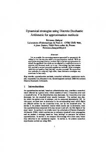
Within each sample path, our algorithm uses the common random numbers and the same sample size for all the design points visited. The sequence of sample-path problems increase sample sizes by 10% each time and use the random initial seed values. We run 10 independent macroreplications with random starting solutions and different initial seeds using our LIS0 algorithm. Figure 1 shows 10 independent simulation runs of our algorithm. The dot-dash line shows the performance of COMPASS solving the same problem. Figure 2 (Hong and Nelson 2006) shows the performance of COMPASS compared to those of simulated annealing and random search. In the inventory example, for the same quality of solution COMPASS requires roughly one-hundred times the computing effort of LISO. COMPASS solves a transient problem but it cannot optimize the steady-state systems. Our algorithm solves the steady-state assembleto-order problem with similar results to those of the transient case presented here. Our LIS0 algorithm finds the optimal solution faster and more efficiently especially for problems with large feasible sets. Figure 3 shows its search path for an assemble-toorder problem with a feasible set of integer vectors [1, 1000]8 which is much larger than the previous instance of problem. Random search methods like COMPASS can be quite slow. Our algorithm finds the optimal solution of problems having

(b) Set s = 2i−1 × s0 ; (c) Set xold = xnew ; ˆ v||; (d) Set xnew = xold + s × v/|| ˆ / Q, project xnew back to Q; (e) If xnew ∈ (f) Simulate at xnew with sample size mk to calculate fˆ(xnew ) = Y mk (xnew , ξk ); (g) If fˆ(xnew ) < fˆ(xold ), go to (a); (v) Step 3

Set xk = xold ; If i > 1, go to Step 2; Iterate:

(i)

Set k = k + 1;

(ii)

Set sample size mk = c × mk−1 ;

(iii)

Set xk = xk−1 ;

(iv)

Go to Step 1;

The above algorithm produces a sequence of continuous solutions {xk } that estimate the true optimal solution of CSP better as the sample size mk goes larger. We can round xk to the closest integer solution or pick the best integer solution from the last RO iteration to get an estimate of the optimal integer solution of ISP.

506

Wang and Schmeiser

180

Estim ated expected profit

180

Estim ated expected profit

160

140

120

compass

100

80

160

140

120

100

60 80 40

20

0

1

2

3

4

5

60

6

x 10

Totalsim ulation tim e

3

4

5

6

x 10 4

REFERENCES

160

Estim ated optim alprofit

2

Figure 3: Optimizing an large assemble-to-order system

170

Andrad´ottir, S. 1998. A review of simulation optimization techniques. Proceedings of the 1998 Winter Simulation Conference:151–158. Biles, W., J. Kleijnen, and I. Nieuwenhuyse. 2007. Kriging metamodeling in constrained simulation optimization: an explorative study. Proceedings of the 2007 Winter Simulation Conference:355–362. Chen, H., and B. Schmeiser. 1994. Retrospective approximation algorithms for stochastic root finding. Proceedings of the 1994 Winter Simulation Conference:255–261. Clarke, F. 1990. Optimization and nonsmooth analysis. Society for Industrial and Applied Mathematics, Philadelphia. Fu, M., F. Glover, and J. April. 2005. Simulation optimization: a review, new developments, and applications. Proceedings of the 2005 Winter Simulation Conference:83–95. Haarala, N., K. Miettinen, and M. M¨akel¨a. 2007. Globally convergent limited memory bundle method for largescale nonsmooth optimization. Math. Program. 109 (1): 181–205. Healy, K., and L. Schruben. 1991. Retrospective simulation response optimization. Proceedings of the 1991 Winter Simulation Conference:901–906. Hiriart-Urruty, J., and C. Lemarechal. 1993. Convex analysis and minimization algorithms I and II. Springer-Verlag. Hong, L. J., and B. L. Nelson. 2006. Discrete optimization via simulation using compass. Operations Research 54 (1): 115–129.

150 140 130 120 110 CO M PA SS sim ulated annealing random search

100 90 80 0

0.5

1.0

1.5

2.0

TotalSim ulation Tim e

2.5

3.0

×7×10 5

Figure 2: Performance of COMPASS (Hong and Nelson 2006) compared to random search and simulated annealing

large solution space with a small increase of computing time.

6

1

Totalsim ulation tim e

Figure 1: Optimizing an assemble-to-order system

70

0

4

SUMMARY

The proposed LIS0 algorithm using linear interpolation gives promising results in our numerical experiments. Convergence analysis and new algorithm design are our future work.

507

Wang and Schmeiser Huang, D., T. Allen, W. Notz, and N. Zeng. 2006. Global optimization of stochastic black-box systems via sequential kriging meta-models. Journal of Global Optimization 34 (3): 441–466. Jin, J., and B. Schmeiser. 2003. Simulation-based retrospective optimization of stochastic systems. Proceedings of the 2003 Winter Simulation Conference:543–547. Kiwiel, K. 1985. Methods of descent for nondifferentiable optimization. Springer-Verlag. Kleywegt, A., A. Shapiro, and T. Homem-De-Mello. 2001. The sample average approximation method for stochastic discrete optimization. SIAM J. Optimization 12 (2): 479–502. Koenig, L., and A. Law. 1985. A procedure for selecting a subset of size m containing the l best of k independent normal populations, with applications to simulation. Comm. in Statist.: Simulation and Comput. 14:719– 734. Kushner, H., and D. Clark. 1978. Stochastic approximation methods for constrained and unconstrained systems. Springer-Verlag, New York. Pichitlamken, J., and B. Nelson. 2003. A combined procedure for optimization via simulation. ACM Trans. Modeling and Comput. Simulation 13:155–179. Rovatti, R., M. Borgatti, and R. Guerrieri. 1998. A geometric approach to maximum-speed n-dimensional continuous linear interpolation in rectangular grids. IEEE Transactions on Computers 47 (8): 894–899. Shapiro, A., and Y. Wardi. 1996. Convergence analysis of gradient descent stochastic algorithms. Journal on Optimization theory and application 91 (2): 439–454. Shor, N. 1985. Minimization methods for non-differentiable functions. Springer-Verlag. Spall, J. 2005. Introduction to stochastic search and optimization, 425–432. John Willey & Sons. Swisher, J., P. Hyden, S. Jacobson, and L. Schruben. 2000. A survey of simulation optimization techniques and procedures. Proceedings of the 2000 Winter Simulation Conference:119–128. Weiser, A., and S. Zarantonello. 1988. A note on piecewise linear and multilinear table interpolation in many dimensions. Mathematics of Computation 50 (181): 189–196.

on developing methods for better simulation experiments. He is a fellow of INFORMS and IIE, and has been active within the Winter Simulation Conference for many years.

AUTHOR BIOGRAPHIES HONGGANG WANG is a PhD candidate in Shool of Industrial Engineering at Purdue University. His research interests include discrete stochastic optimiztion via simulation, stochastic process and modeling, and stochastic optimization in supply chain management. BRUCE W. SCHMEISER is a professor of Industrial Engineering at Purdue University. His research interests center

508