Copyright © IFAC Large Scale Systems: Theory and Applications. Bucharest. Romania. 200 I
DISCRETE-TIME LINEAR-QUADRATIC OUTPUT REGULATOR FOR MULTIVARIABLE SYSTEMS Ryszard Gessing
Politechnika Sll}ska Instytut Automatyki, ul. Akademicka 16, 44-101 Gliwice, Poland, lax: +4832 372127, email:
[email protected]
Abstract: It is shown, that in discrete-time multi-variable systems, the usual observers used with the state feedback law of the LQ regulator are optimal for some adequate initial condition. It is also shown, that for the systems with stepwise excitations of the plant outputs, the optimal LQ regulator results from the Deterministic Equivalence Principle, formulated and proved in the paper. The principle says that the optimal regulator results from substituting in the LQ state control law the state estimate obtained from the reduced order, Luenberger observer. Both the problems: control and observer may be solved separately. Copvrighl @20011FAC Keywords: Linear-quadratic regulator; discrete-time systems; multi-variable systems.
1. INTRODUCTION
tor with output feedback is optimal? The case of discrete-dime linear-quadratic regulator (DLQR) problem with output feedback, for multi-variable systems is considered.
Linear-Quadratic Regulator (LQR) problem, in infinite horizon, has usually the solution in the form of a static state feedback control law and may be implemented when all the state variables are available (Dorato et al., 1995) . This observation concerns continuous- and discrete-time, as well as single- and multi-variable plants. When only the outputs of the plant are measured, the state feedback LQ control law may be implemented, if an appropriate state observer IS Included in the system (Astrom, 1997).
It is noted that the usual observers are optimal for adequate initial conditions. It is shown, that for the system with stepwise excitations of the plant outputs, the optimal regulator based on the reduced order observer results from the Deterministic Equivalence Principle (DEP). The latter says that the optimal regulator results from substituting in the DLQR state control law the state estimate obtained from the reduced order, Luenberger observer. The principle corresponds to the known Certainty Equivalence Principle valid for some stochastic systems (Bar-Shalom and Tse, 1974) . The shown property may be also called the Separation Principle since the optimal regulator results from separate solving the DLQR problem with state feedback and the reduced order observer problem.
In H2 approach the optimal observers are considered for which the observer based regulators are H2 optimal (Saberi et al., 1995). But this approach is related with very cumbersome derivations and also with higher concept and calculation difficul ties. In the present paper the following question is researched: whether, and when the usual observers applied with LQ state feedback law are optimal, or whether and when the observer -based LQ regula551
The dosed-loop (CL) system (1), (4) is described by
Similar results were obtained in (Gessing, 2001) for plants with single input and single output. In this case the design procedure of the optimal regulator may be obtained using the polynomial methods.
x(t
+ 1) = (A - BK)x(t)
(7)
with the characteristic equation The contribution of the paper is in showing that the optimal DLQR with output feedback, in the multivariable system with stepwise excitations of the plan outputs, results from the Deterministic Equivalence Principle.
det(zI - A
y(t)
(8)
3. OBSERVER BASED REGULATOR The control law (4) may be implemented if all the state components are available (measured). Further on, the case when only the output variable y is available will be considered. It is known that in this case the control law (4) may be implemented if an appropriate observer estimating the state is applied.
Let the state space model of a discrete-time (DT) multi-variable plant takes the form
= Ax(t) + Bu(t),
= O.
Let AI, A2, ... , An be the poles of the CL system (7) . Of course they are determined by the roots of the characteristic equation (8).
2. LQ REGULATOR WITH STATE FEEDBACK
x(t + 1)
+ BK)
= Cx(t) (1)
where x, u and y are the vectors of state, input and output, n, r and p-dimensional, respectively; A, B, C are constant matrices of appropriate dimension; t = 0,1,2, ... is the discrete time.
3.1 Reduced Order Observer
The plant (1) may be also described by the matrix transfer function (MTF). G(z)
= C(zIn -
A)-l B
The equations of the reduced order (Luenberger) observer for the plant (1) have the form (Saberi et al., 1995):
(2)
v(t
where In is the unit n x n matrix. Let the quadratic performance index takes the form
= ~)XI(t)QX(t) +u'(t)Ru(t»),
(9)
= Vv(t) + Wy(t)
(10)
x(t)
where x(t) and v(t) are the vectors of the plant state and observer state estimates, n and mdimensional respectively, m = n-p; E,F,G, V, W are the constant matrices of appropriate dimension such that IXil < 1, i = 1,2, ... , m where Xi are the eigenvalues of E and there exists a m x n matrix T fulfilling the equations
N
J
+ 1) = Ev(t) + Fy(t) + Gu(t)
N -+ 00(3)
t=o
where the symmetric matrices Q = D' D and R are semipositive and positive definite, respectively. Assume, that the pair (A, B) is controlable and the pair (A, D) is observable.
TA-ET=FC
(ll)
G=TB
(12)
WC+ VT = In.
(13)
The solution of the DLQR problem (1), (3) in the form of the state feedback is u(t)
= -Kx(t)
(4)
where the gain matrix K is determined by
K
= (R+ B SB)-IB SA I
I
To explain this, denote
(5)
and S is the solution of the algebraic Riccati equation
S
= Q + A'SA -
v=Tx
(14)
Multiplying both sides of (1) by T from left hand side and accounting (1l)-(13), (1), (14) we obtain
A'SB(R+ B I SB)-1 B ' SA(6) 552
vet + 1)
= Ev(t) + Fy(t) + Gu(t)
x(t) = Vv(t)
+ Wy(t)
(15)
3.2 Full Order ObsenJer
(16)
The full order observer is described by the equations (9), (la) in which
Neither vet) nor x(t) are known but vet) ~ vet) when t ~ 00. Thus vet) determines the estimate of vet) and the equations (9), (10) determine the reduced order observer. Note that it is a freedom in choosing matrices E, F (and eigenvalues Xi) which guaranties the fast observer convergence.
E=A-FC, G=B, V=[n, W=O, m=n
Therefore vet) == x(t) and observer is of n-th order. For the observable plant (1) there exists the matrix F such that the poles Xi> i = 1,2, ... , n may be placed, freely. The CL system (18) with the regulator based on the full order observer is of 2n-th order and has the poles being the eigenvalues of (A - BK) and of (A - FC).
The CL system with dynamic output feedback LQ regulator (DOFR) which may be implemented when only the output y is available is described by (1), (9), (10) with accounting u(t) == -Kx(t)
The MTF of the regulator based on the full order observer takes the form
(17)
After transformations we obtain x(t + 1) == (A - BK)x(t) v(t + 1) = EiJ(t)
+ BKVv(t)
R(z) (18)
= vet) -
vet)
(19)
From the form of (18) the known fact results, that the CL system with DOFR is of (n + m)-th-order and has the poles AI, A2, ... , An, Xl, X2, ... , Xm being the union of the poles of the system (7) with LQ regulator and state feedback and of the observer (9), (10).
+ 1) = (E - GKV)v(t) +
= -KVv(t) -
+ FC + BK)-l F
(24)
One can suppose that the reduced order observer (9), (10) determines the accurate estimate of the state (Le. x(t) = x(t» if the initial condition V(O) of the observer is adequate to the initial condition x(O) of the plant state. Note, that the formula (16) determines the transformation of the state [v T yT]T to the state x, which may be written in the form
(20)
+(F - GKW)y(t) u(t)
A
4. WHETHER AND WHEN THE OBSERVER IS OPTIMAL?
The state space equations of the regulator, based on the reduced order observer, result from (9), (la) and (17) and take the form vet
= -K(zI -
The form of the MTF (24), resulting from the fact that W = 0, means that the regulator has one step (sampling period) delay in its time response. This fault disappears in the regulator (21) . Additionally the CL system with full order observer has a higher order. All this speaks rather for using the reduced order observer.
where vet)
(23)
KWy(t)
The resulting matrix transfer function (MTF) of the regulator takes the form
(25)
R(z)=-KV(z[-E+GKV)-1(F-GKW)-(21)
Accounting (13) we obtain the inverse transformation in the form
-KW
(26)
The output feedback is described by U(z)
= R(z)Y(z)
(22)
Lemma 1. Optimality of the Observer. For the initial conditions x(O), V(O) fulfilling the relation
where U(z) and Y(z) are Z-transformsofu(t) and yet), respectively.
553
iI(O)] _ [T] (0) [ y(O) - C x
important role in some CL systems for stepwise excitations of the plant output. To formulate this property in details, consider the CL system shown in Fig. 1 which stabilizes the disturbed output Yl on the level determined by the set point w. The system is excited by
(27)
the reduced order observer (9), (10) applied with the LQ control law (17) to the plant (1) is optimal in the sense that in the resulting CL system the performance index achieves the optimal value equal to that ofthe CL system (1), (4) with DLQR and state feedback.
w(t)
When t ~ 00 there arises a steady state in the CL system. Let es , Us, x s , Vs, Ys denote the values of the variables e, u, x, iI, y, respectively, in this steady state. Note, that from the assumptions concerning the poles of the observer and of the CL system it results that the values of the mentioned variables in steady state are determined, uniquely.
The initial condition iI(O) determined by (27) is called the adequate initial condition of the observer. To implement the optimal control in the CL system (1), (9), (10), (17) the initial condition x(O) of the plant must be determined. The adequate initial condition iJ(O) of the observer results from (27).
Consider the performance index in the form
Corollary 1, below, determines the special case of the initial conditions of the CL system which will be interesting from application point of view.
DO
j = L[xT(t
= Wy(O),
+ I)Qx(t + 1) + u'(t)Ru(t)] (30)
t=O
wherex(t) = x(t)-x s andu(t) = u(t)-u s denote the increases of x and u from steady state values Xs and us ·
Corollary 1. Lemma 1 is also valid for the special case of initial conditions x(O) xo, iI(O) = 0, fulfilling the relation
[y~O)]
(29)
where 1 (t) denotes the unit step function, and d· ,w· are the constant p-dimensional vectors, components of which determine the disturbances and set points for particular m outputs of the plant. Note that in the system shown in Fig. 1 the input of the regulator is e (but not y), which should be taken into account in observer equations (9), (10).
Proof. From (26) and (27) it results that iI(O) = v(O), then ii(O) = 0 and from (18) we obtain ii(t) = 0 which gives iI(t) = v(t) for any t > o. Accounting (10) and (16) we obtain x(t) = x(t) for any t > o. Therefore the formula (17) determines the optimal control of the CL system with DLQR and state feedback.
xo = [V W]
= w·1(t)
Theorem 1. Deterministic Equivalence Principle (DEP). The optimal regulator TF R(z) , which for step wise excitations (29) of the plant output shown in Fig. 1, minimizes the performance index (30), is determined by (21) and results from substituting in the LQ control law (17), the state estimate x(t) obtained from the reduced order, Luenberger observer (9), (10).
iI(O) = 0 (28)
where y(O) takes any value taken from the set of real numbers.
Proof. As the input of the regulator R(z) shown in Fig. 1 is e (but not y), the equations (15), (16) and (4), now, take the form
J2.(t Fig. 1. Closed loop system.
+ 1) =
EJ2.(t)
~(t) =
5. DETERMINISTIC EQUVALENCE PRINCIPLE
+ Fe(t) + Gu(t)
VJ2.(t)
u(t)
+ We(t)
= -K~(t)
(31)
(32)
(33)
where ~(t) = x(t) - Xdw, J2.(t) v(t) Vdw ; Xdw, Vdw are some ve