The first sequence is the `Yosemite' sequence.5 True optical flow vectors were ... Sample image from the Yosemite sequence A and the angular error metric of.
Presented at: 7th Int'l Conf Computer Analysis of Images and Patterns, Kiel, Germany. September 10-12, 1997.
Discrete-Time Rigidity-Constrained Optical Flow? Je�rey Mendelsohn1 , Eero Simoncelli2 , and Ruzena Bajcsy1 1
University of Pennsylvania, Philadelphia PA 19104-6228, USA 2 New York University, New York NY 10003-6603, USA
Abstract. An algorithm for optical ow estimation is presented for the
case of discrete-time motion of an uncalibrated camera through a rigid world. Unlike traditional optical ow approaches that impose smoothness constraints on the ow eld, this algorithm assumes smoothness on the inverse depth map. The computation is based on di�erential measurements and estimates are computed within a multi-scale decomposition. Thus, the method is able to operate properly with large displacements (i.e., large velocities or low frame rates). Results are shown for a synthetic and a real sequence.
1 Introduction Estimation of optical ow, a longstanding problem in computer vision, is particularly di�cult when the displacements are large. Multi-scale algorithms can handle large image displacements and also improve overall accuracy of optical
ow elds [1, 5, 9, 15]. However, these techniques typically make the unrealistic assumption that the ow eld is smooth. In many situations, a more plausible assumption is that of a rigid world. Given point and/or line correspondences, the discrete-time rigid motion problem has been studied and solved by a number of authors (e.g. [6, 7, 11, 14, 17]). For instantaneous representations, multi-scale estimation techniques have been used to couple the ow and motion estimation problems to provide a direct method for planar surfaces [4, 8]. These methods use the multi-scale technique to capture large motions while signi cantly constraining the ow with a global model. But the planar world assumption is quite restrictive, and the approach also contains a hidden contradiction; the algorithm can observe large image motions but can only represent small camera motions due to the instantaneous time assumption. ?
J. Mendelsohn is supported by NSF grant GER93-55018. R. Bajcsy is supported by ARO grant DAAH04-96-1-0007, ARPA grant N00014-92-J-1647, and NSF grants IRI93-07126 and SBR89-20230. E. Simoncelli is supported by NSF CAREER grant MIP-9796040, the Sloan Center for Theoretical Neurobiology at NYU, and ARO/MURI grant DAAH04-96-1-0007 to UPenn/Stanford.
This paper describes an optical ow algorithm for discrete camera motion in a rigid world. The algorithm is based on di�erential image measurements and estimates are computed within a multi-scale decomposition; the estimates are propagated from coarse to ne scales. Unlike traditional coarse-to- ne approaches which impose smoothness on the ow eld, this algorithm assumes smoothness of the inverse depth values.
2 Discrete-Time Optical Flow The imaging system is assumed to use the following projection model: 1
p = Cx z
2x 3 x � 4y 5 i
i
i
z
i
and
i
; (1) 1 x denotes the point's coordinates in the camera's frame of reference and p the image coordinates. The matrix C contains the camera calibration parameters and is presumed invertible.3 The discrete motion of a point is expressed as: x = Rx + t ; (2) where R is a (discrete-time) rotation matrix, t is a translation vector, and x denotes the point's coordinates after the discrete motion. A classic formulation of this constraint is due to Longuet-Higgins [10]: x (t � Rx ) = 0 : Using equation (1) to substitute for x gives: z0p (C ,1) ,t � RC,1p z � = 0 : (3) i
where
2u 3 p � 4v 5
i
i
i
i
i
i
0
i
i
0
0T
i
i
i
i
0T
i
0
T
i
i
i
Let t� represent the skew-symmetric matrix corresponding to a cross-product with t. Using suitable linear algebraic identities, and assuming that z 6= 0 and z0 6= 0, leads to the following simpli cation: 0 = z 0 p (C ,1 ) t� RC,1 p z 0 = p (C ,1 ) t� C ,1 C RC,1 p 0 = p (C t)� C RC,1 p 0 = p Lp ; (4) where L � (C t)� C RC,1 is a matrix that depends on the global motion and camera calibration information. Equation (4) provides a constraint on the initial i
i
0T
i
0
i
0T
0
T
i
0
T
0
i
0T i
0T i
0
3
0
0
i
i
i
i
0
This assumption is valid for any reasonable camera system. For example, the pinhole model is included in this family, as well as more complex models such as that given in [16].
2
and nal image positions assuming rigid-body motion and is, essentially, the fundamental matrix [12]. In addition, it will be useful to develop an expression for the nal position, p , given the calibration, motion, and structure parameters. Substituting the inverse of equation (1) into the rigid-body motion constraint of equation (2): 0
i
C , p z0 = RC, p z + t : 1
0
0
i
1
i
i
i
Solving for the image position after the motion: , p = C� RC ,p + C t � ^z C RC p + C t 1
0
0
i
0
T
1
1
0
i
zi
1
0
i
203 ^z = 4 0 5 :
where
(5)
1
zi
This rigid-world motion constraint must be connected with measurements of image displacements. Since di�erential optical ow techniques have proven to be quite robust [2], the formulation is based on the di�erential form of the `brightness constancy constraint' [8]:
@I � @u + @I � @v + @I = 0 : @u @t @v @t @t i
i
i
i
i
Substituting discrete displacements for the di�erential changes in image positions4 and rewriting to isolate p0 gives: i
2 @I=@u 3 2 u0 , u 3 2 @I=@u 3 2 4 @I=@v 5 4 v0 , v 5 = 4 @I=@v 5 4 T
@I=@t
1 0 0
T
i
i
i
i
1
@I=@t
i
i
0 ,u 1 ,v 0 1
i
i
3 5 p0 = 0 :
(6)
i
This constraint is combined with equation (5), squared, and summed over a local neighborhood, N (i), to produce an error metric:
� � � � Ap + b D Ap + b ; E (A; b; z1 ) = � � ^z Ap + ^z b where A � C RC, , b � C t, and D is a matrix constructed from the di�erential image measurements and known position vectors: 2 1 0 ,u 3 0 2 @I=@u 3 2 @I=@u 3 1 2 1 0 ,u 3 X 4 @I=@v 5 4 @I=@v 5 CA 4 0 1 ,v 5 ; D � 4 0 1 ,v 5 B @ 1
i
T
i
zi
i
i
T
1
0
0
i
1
i
T
1
zi
2
zi
i
T
T
i
i
4
0
0
1
i
i
j
2
N (i)
@I=@t
j
@I=@t
j
0
0
1
i
The displacements are assumed to be small; this is reasonable given the multi-scale (coarse-to- ne) framework described in Section 3.
3
Minimizing E (A; b; 1 ) with respect to i
zi
,
gives:
1
zi
�
p A D I , b^z Ap 1 z = , b D (I , b^z ) Ap T i
T
T
i
i
T
i
:
i
T
i
Substituting back into E (A; b; 1 ), and noting that L = b� A: i
zi
)� D Ap : E (A; b) = , b D (Lp (Lp ) (^z� ) D ^z� (Lp ) T
i
i
i
T
i
T
i
i
i
i
Using a series of linear algebraic manipulations, the numerator may be rewritten as an expression quadratic in L: ,(D b) (Lp )� D Ap = (Lp ) (D b)� D Ap = jD j(Lp ) D,1 b� Ap = jD j(Lp ) D,1 Lp ; where jD j indicates the determinant of the matrix D . To e�ciently solve for L, a global metric is formed by summing over the image the weighted numerators of the E (A; b): i
T
i
i
i
i
T
i
i
i
i
i
i
i
i
T
i
i
T
i
i
i
X i
E (A; b) =
jD j(Lp ) D, Lp =w ; i
i
1
T
i
i
(7)
i
i
where w is the value of the denominator of E (A; b) using the previous estimate of L. This metric is computed iteratively in the coarse-to- ne procedure and, from empirical observations, only one iteration at each scale is necessary. The algorithm proceeds by rst globally minimizing equation (7) to obtain a solutionPforPthe nine entries of the matrix L, subject to the constraints jLj = 0 and (L )2 = 1 (to remove the scale ambiguity). Then, the squared optical ow constraint E (p ) = p D p ; (8) is minimized at each pixel, subject to equation (4) with the estimated value of L, to obtain an optical ow eld. i
i
j
i
j;i
f
0
0T
i
i
i
0
i
3 Multi-Scale Implementation Since the method is capable of estimating large (discrete) camera motions, it must be able to handle large image displacements. This is accomplished with a coarse-to- ne version of the algorithm on a multi-scale decomposition. First, a Gaussian pyramid is constructed on the pair of input frames [3]. At the coarsest scale of the pyramid, the algorithm is employed as derived in the previous section to provide an initial coarse estimate of optical ow. This optical
ow is interpolated to give a ner resolution ow eld, denoted (� u ; � v ). This c
4
i
c
i
motion is removed from the ner scale images using warping; the warped images are denoted I . Since the optical ow equation (8) is written only in terms of the nal positions p , the constraint on the warped images needs only a slight modi cation: 2 @I =@u 3 2 1 3 0 ,(u + � u ) 4 @I =@v 5 4 0 1 ,(v + � v ) 5 p0 = 0 : @I =@t 0 0 1 The remainder of the algorithm is as before: new matrices D are computed from this constraint and these are used to estimate L using equation (7). The weightings, w , are computed using the estimate of L from the previous scale. Finally, equation (8) is minimized at each pixel, subject to the constraint of equation (4), to estimate the optical ow. w
0
i
w
T
c
i
w
c
i
w
i
i
i
i
i
i
4 Experimental Results Experimental results were collected for three di�erent algorithms on two sequences. The rst method is a simple multi-scale optical ow (msof) algorithm [15]. The second computes ow for discrete motion of a planar world (planar) [13]. The third is the algorithm presented in this paper (rigid). The rst sequence is the `Yosemite' sequence.5 True optical ow vectors were computed from the motion, structure, and calibration data provided with the sequence. The textureless top region was ignored during error calculations. In order to obtain large motions, the computations are performed on the sequence subsampled at di�erent temporal rates. The second sequence was taken in the GRASP Laboratory from a camera mounted on a tripod. Six markers consisting of seven black disks on a white planar surface were placed in the scene and used to calculate ground-truth. Using knowledge of the individual targets, accurate centroids for the disks were computed. Flow was calculated from the motion of each centroid for a total of 42 ow vectors. Table 1 shows results. The metric is the mean angular error in degrees [2]: X E = 1 cos,1(v^ v^ ) n
a
n
T ti
ei
i=1
where v^ is a unit three-vector in the direction of the true ow and v^ is a unit three-vector in the direction of the estimated ow. The multi-scale optical ow algorithm did well for small motions but poorly for large ones. Since the range map for the Yosemite sequence is nearly planar, the di�erence in performance between the discrete algorithms is less signi cant than those for the real sequence. It is clear that the rigid algorithm provides the best optical ow estimates. ti
5
ei
This sequence was graphically rendered from an aerial photograph and range map by Lyn Quam at SRI.
5
sequence ! frame interval !
msof planar rigid
1
6.13o 5.82o 5.77o
2
7.49o 6.56o 5.86o
3
13.10o 6.70o 6.18o
Yosemite 4 5 21.32o 6.70o 6.53o
29.09o 6.92o 6.55o
6
35.82o 6.82o 6.77o
7
42.43o 7.63o 6.95o
Table 1. Mean angular error in ow vectors for three di�erent algorithms. See text.
A
B
C
D
Fig. 1. Sample image from the Yosemite sequence (A) and the angular error metric of
the computed ow elds for the Yosemite sequence by the msof (B), planar (C), and rigid (D) algorithms with a frame interval of four. White corresponds to 0o of error and black to 45o .
5 Conclusion A multi-scale algorithm for estimating optical ow based on an uncalibrated camera moving through a rigid world has been presented. Its implementation is only slightly more complicated and time-consuming than standard multi-scale algorithms. In situations where the camera may be undergoing relatively large motions, the superiority of the rigid model has been demonstrated on both a synthetic and a real sequence.
References 1. P. P. Anandan. A Computational Framework and an Algorithm for the Measurement of Visual Motion. IJCV, 2, 283{310, 1989.
6
Real 1 3.28o 2.87o 2.05o
A
B
C
D
Fig. 2. True ow eld (A) and computed ow elds for the Yosemite sequence by the msof (B), planar (C), and rigid (D) algorithms with a frame interval of four. 2. J. L. Barron, D. J. Fleet, and S. S. Beauchemin. Performance of Optical Flow Techniques. IJCV, 1992. 3. P. J. Burt. Fast lter transforms for image processing. Computer Graphics and Image Processing, 16, 20{51, 1981. 4. J.R. Bergen, P. Anandan, K.J. Hanna, and R. Hingorani. Hierarchical ModelBased Motion Estimation. Proc. ECCV, 237{252, Springer-Verlag, Santa Margherita Ligure, Italy, 1992. 5. W. Enkelmann and H. Nagel. Investigation of Multigrid Algorithms for Estimation of Optical Flow Fields in Image Sequences. Computer Vision Graphics Image Processing, 43, 150{177, 1988. 6. R. Hartley. Projective Reconstruction from Line Correspondences. Proc. IEEE CVPR, 1994. 7. R. Hartley, R. Gupta, and T. Chang. Stereo from Uncalibrated Cameras. Proc. IEEE CVPR, 1992. 8. B.K.P. Horn. Robot Vision. MIT Press, Cambridge, MA, 1986. 9. M. Leuttgen, W. Karl, and A. Willsky. E�cient Multiscale Regularization with Applications to the Computation of Optical Flow. IEEE Trans. Im. Proc., 1992. 10. H. C. Longuet-Higgins and K. Prazdny. The interpretation of a moving retinal image. Proc. Royal Society of London B, 208, 385{397, 1980.
7
A
B
C
D
Fig. 3. Sample image from the real sequence (A) and the computed ow elds for the real sequence by the msof (B), planar (C), and rigid (D) algorithms.
11. Q.T. Luong and T. Vieville. Canonic Representation for the Geometry of Multiple Projective Views. Proc. ECCV, Stockholm, 1994. 12. Q.T. Luong and O. Faugeras. The Fundamental Matrix: Theory, Algorithms, and Stability Analysis. IJCV, 43{76, 1996. 13. J. Mendelsohn, E. Simoncelli, and R. Bajcsy. Discrete-Time Rigid Motion Constrained Optical Flow Assuming Planar Structure. Univ. of PA GRASP Laboratory Technical Report #410, 1997. 14. A. Shashua and N. Navab. Relative A�ne Structure: Theory and Application to 3D Reconstruction from Perspective Views. Proc. IEEE CVPR, Seattle, June 1994. 15. E. P. Simoncelli, E. H. Adelson, and D. J. Heeger. Probability Distributions of Optical Flow. Proc. IEEE CVPR, Maui, June 1991. 16. T. Vieville and O. D. Faugeras. The First Order Expansion of Motion Equations in the Uncalibrated Case. Computer Vision and Image Understanding, 128{146, July 1996. 17. T. Vieville, C. Zeller, and L. Robert. Using Collineations to Compute Motion and Structure in an Uncalibrated Image Sequence. IJCV, 1995. This article was processed using the LATEX macro package with LLNCS style.
8