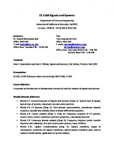
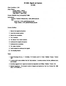
Chapter 2: Discrete-Time Signals and Systems. Discrete-Time Signals and
Systems. Reference: Sections 2.1 - 2.5 of. John G. Proakis and Dimitris G.
Manolakis, ...
Chapter 2: Discrete-Time Signals and Systems
Discrete-Time Signals and Systems
Discrete-Time Signals and Systems
Reference: Sections 2.1 - 2.5 of
Dr. Deepa Kundur
John G. Proakis and Dimitris G. Manolakis, Digital Signal Processing: Principles, Algorithms, and Applications, 4th edition, 2007.
University of Toronto
Dr. Deepa Kundur (University of Toronto)
Discrete-Time Signals and Systems
1 / 36
Dr. Deepa Kundur (University of Toronto)
Chapter 2: Discrete-Time Signals and Systems
Discrete-Time Signals and Systems
2 / 36
Chapter 2: Discrete-Time Signals and Systems
Elementary Discrete-Time Signals
Signal Symmetry
1. unit sample sequence (a.k.a. Kronecker delta function): � 1, for n = 0 δ(n) = 0, for n 6= 0
Even signal:
x(−n) = x(n)
Odd signal: x(−n) = −x(n) 2. unit step signal: � u(n) =
1, 0,
for n ≥ 0 for n < 0
� ur (n) =
n, for n ≥ 0 0, for n < 0 -7
Note: δ(n)
x(n)
x(n)
2
2
2
1
1
1
x(n)
3. unit ramp signal:
-6
-5
-4
-3
-2
-1
0
1
2
3
4
5
6
7
n
-7
-6
-5
-4
-3
-2
-1
0
1
2
3
4
5
6
7
n
-7
-6
-5
-4
-3
-2
-1
0
1
2
3
4
5
6
7
= u(n) − u(n − 1) = ur (n + 1) − 2ur (n) + ur (n − 1)
u(n) = ur (n + 1) − ur (n) Dr. Deepa Kundur (University of Toronto)
Discrete-Time Signals and Systems
3 / 36
Dr. Deepa Kundur (University of Toronto)
Discrete-Time Signals and Systems
4 / 36
n
Chapter 2: Discrete-Time Signals and Systems
Chapter 2: Discrete-Time Signals and Systems
Signal Symmetry
Signal Symmetry 1
x(n)
(x(n)+x(-n))/2 1
0.5
1 2
Even signal component: xe (n) = [x(n) + x(−n)]
-6 -5 -4 -3 -2 -1 0 1
-0.5
Odd signal component: xo (n) = 12 [x(n) − x(−n)]
2 3 4
5 6
7 8
n
-6 -5 -4 -3 -2 -1 0 1
-0.5
-1
Note: x(n) = xe (n) + xo (n)
1
0.5 -6 -5 -4 -3 -2 -1 0 1
5 / 36
Chapter 2: Discrete-Time Signals and Systems
n
7 8
2 3 4
5 6
7 8
n
-6 -5 -4 -3
-2 -1
-1
Dr. Deepa Kundur (University of Toronto)
odd part
0.5
-1
Discrete-Time Signals and Systems
5 6
(x(n)-x(-n))/2
1
Dr. Deepa Kundur (University of Toronto)
2 3 4
-1
x(-n)
-0.5
even part
0.5
0 1
2 3 4
-0.5
5 6
n
7 8
Discrete-Time Signals and Systems
6 / 36
Chapter 2: Discrete-Time Signals and Systems
Simple Manipulation of Discrete-Time Signals
Simple Manipulation of Discrete-Time Signals I Find x(n) − x(n + 1).
I
Transformation of independent variable: I
time shift: n → n − k, k ∈ Z I
I
2
time scale: n → αn, α ∈ Z I
I
3
Question: what if k 6∈ Z? Question: what if α 6∈ Z?
I I
3 2
2
1
1
Additional, multiplication and scaling: I
x(n)
-3 -2 -1 0 1
amplitude scaling: y (n) = Ax(n), −∞ < n < ∞ sum: y (n) = x1 (n) + x2 (n), −∞ < n < ∞ product: y (n) = x1 (n)x2 (n), −∞ < n < ∞
-1
2 3 4
5 6
7 8 9 10
Discrete-Time Signals and Systems
7 / 36
Dr. Deepa Kundur (University of Toronto)
20
n
-1
-2
-2
-3
Dr. Deepa Kundur (University of Toronto)
15
Discrete-Time Signals and Systems
8 / 36
Chapter 2: Discrete-Time Signals and Systems
Chapter 2: Discrete-Time Signals and Systems
Simple Manipulation of Discrete-Time Signals II
Simple Manipulation of Discrete-Time Signals I Find x( 32 n + 1).
x(n)
3
2
1
1 -3 -2 -1 0 1
-1 -1 -2
2 3 4
-1
5 6
2
1
n < −1 -1 0 1 2 3 4 5 6 7 8 9 10 11 12 > 12
x(n)-x(n+1) 1 15
7 8 9 10
20
n
-1
-1
-3 -x(n+1)
Dr. Deepa Kundur (University of Toronto)
Discrete-Time Signals and Systems
9 / 36
3
2
-1
3n 2
0 if
3n 2
5 2
4 11 2
7
17 2
10 23 2
13 29 2
16 35 2
19 > 19
x( 3n + 1) 2 + 1 is an integer; undefined otherwise undefined x(1) = 1 undefined x(4) = 2 undefined x(7) = 3 undefined x(10) = 2 undefined x(13) = 1 undefined x(16) = −1 undefined x(19) = −2 + 1 is an integer; undefined otherwise
Discrete-Time Signals and Systems
10 / 36
Input-Output Description of Dst-Time Systems
+ 1). input/ excitation
3 2
2
1
1 -3 -2 -1 0 1
0 if
Chapter 2: Discrete-Time Signals and Systems
Simple Manipulation of Discrete-Time Signals Graph of
+1 < − 12 − 12 1
Dr. Deepa Kundur (University of Toronto)
Chapter 2: Discrete-Time Signals and Systems
x( 23 n
3n 2
2 3 4
-2 -3
Dr. Deepa Kundur (University of Toronto)
5 6
This signal is undefined for values of n that are not even integers and zero for even integers not shown on this sketch.
7 8 9
10
11
12
13 14
x(n)
Discrete-time System
I
Input-output description (exact structure of system is unknown or ignored): y (n) = T [x(n)]
I
“black box” representation:
-1 -2
output/ response
Discrete-time signal
Discrete-time signal
n
y(n)
T
x(n) −→ y (n) Discrete-Time Signals and Systems
11 / 36
Dr. Deepa Kundur (University of Toronto)
Discrete-Time Signals and Systems
12 / 36
Chapter 2: Discrete-Time Signals and Systems
Chapter 2: Discrete-Time Signals and Systems
Classification of Discrete-Time Systems
Time-invariant vs. Time-variant Systems
Why is this so important? I
I
mathematical techniques developed to analyze systems are often contingent upon the general characteristics of the systems being considered for a system to possess a given property, the property must hold for every possible input to the system I I
I
I
T
Discrete-Time Signals and Systems
for every input x(n) and every time shift k.
13 / 36
Dr. Deepa Kundur (University of Toronto)
Chapter 2: Discrete-Time Signals and Systems
Discrete-Time Signals and Systems
14 / 36
Chapter 2: Discrete-Time Signals and Systems
Time-invariant vs. Time-variant Systems
Linear vs. Nonlinear Systems
Examples: time-invariant or not? I y (n) = A x(n) I y (n) = n x(n) p I y (n) = x(n) + x 2 (n − 2) I y (n) = x(−n) I y (n) = x(n + 1) 1 I y (n) = 1−x(n+2) I
T
x(n) −→ y (n) =⇒ x(n − k) −→ y (n − k)
to disprove a property, need a single counter-example to prove a property, need to prove for the general case
Dr. Deepa Kundur (University of Toronto)
Time-invariant system: input-output characteristics do not change with time a system is time-invarariant iff
I I
Linear system: obeys superposition principle a system is linear iff T [a1 x1 (n) + a2 x2 (n)] = a1 T [x1 (n)] + a2 T [x2 (n)] for any arbitrary input sequences x1 (n) and x2 (n), and any arbitrary constants a1 and a2
y (n) = e 3x(n) Ans: Y, N, Y, N, Y, Y, Y
Dr. Deepa Kundur (University of Toronto)
Discrete-Time Signals and Systems
15 / 36
Dr. Deepa Kundur (University of Toronto)
Discrete-Time Signals and Systems
16 / 36
Chapter 2: Discrete-Time Signals and Systems
Chapter 2: Discrete-Time Signals and Systems
Linear vs. Nonlinear Systems
Causal vs. Noncausal Systems
Examples: linear or not? I y (n) = A x(n) I y (n) = n x(n) p I y (n) = x(n) + x 2 (n − 2) I y (n) = x(−n) I y (n) = x(n + 1) 1 I y (n) = 1−x(n+2) I
y (n) = e
I
I
Causal system: output of system at any time n depends only on present and past inputs a system is causal iff y (n) = F [x(n), x(n − 1), x(n − 2), . . .] for all n
3x(n)
Ans: Y, Y, N, Y, Y, N, N
Dr. Deepa Kundur (University of Toronto)
Discrete-Time Signals and Systems
17 / 36
Dr. Deepa Kundur (University of Toronto)
Chapter 2: Discrete-Time Signals and Systems
Stable vs. Unstable Systems
Examples: causal or not? I y (n) = A x(n) I y (n) = n x(n) p I y (n) = x(n) + x 2 (n − 2) I y (n) = x(−n) I y (n) = x(n + 1) 1 I y (n) = 1−x(n+2) y (n) = e
18 / 36
Chapter 2: Discrete-Time Signals and Systems
Causal vs. Noncausal Systems
I
Discrete-Time Signals and Systems
I
I
Bounded Input-Bounded output (BIBO) Stable: every bounded input produces a bounded output a system is BIBO stable iff |x(n)| ≤ Mx < ∞ =⇒ |y (n)| ≤ My < ∞ for all n.
3x(n)
Ans: Y, Y, Y, N, N, N, Y
Dr. Deepa Kundur (University of Toronto)
Discrete-Time Signals and Systems
19 / 36
Dr. Deepa Kundur (University of Toronto)
Discrete-Time Signals and Systems
20 / 36
Chapter 2: Discrete-Time Signals and Systems
Chapter 2: Discrete-Time Signals and Systems
Stable vs. Unstable Systems
The Convolution Sum
Examples: stable or not? I y (n) = A x(n) I y (n) = n x(n) p I y (n) = x(n) + x 2 (n − 2) I y (n) = x(−n) I y (n) = x(n + 1) 1 I y (n) = 1−x(n+2) I
Recall:
∞ X
x(n) =
x(k)δ(n − k)
k=−∞
y (n) = e 3x(n) Ans: Y, N, Y, Y, Y, N, Y
Dr. Deepa Kundur (University of Toronto)
Discrete-Time Signals and Systems
21 / 36
Chapter 2: Discrete-Time Signals and Systems
Dr. Deepa Kundur (University of Toronto)
Discrete-Time Signals and Systems
22 / 36
Chapter 2: Discrete-Time Signals and Systems
The Convolution Sum
The Convolution Sum
Let the response of a linear time-invariant (LTI) system to the unit sample input δ(n) be h(n). Therefore,
T
δ(n) −→ h(n) T
δ(n − k) −→ h(n − k)
y (n) =
T
α δ(n − k) −→ α h(n − k)
∞ X
x(k)h(n − k) = x(n) ∗ h(n)
k=−∞
T
x(k) δ(n − k) −→ x(k) h(n − k) ∞ ∞ X X T x(k)δ(n − k) −→ x(k)h(n − k) k=−∞
for any LTI system.
k=−∞ T
x(n) −→ y (n)
Dr. Deepa Kundur (University of Toronto)
Discrete-Time Signals and Systems
23 / 36
Dr. Deepa Kundur (University of Toronto)
Discrete-Time Signals and Systems
24 / 36
Chapter 2: Discrete-Time Signals and Systems
Chapter 2: Discrete-Time Signals and Systems
Properties of Convolution
Properties of Convolution
Associative and Commutative Laws:
Distributive Law:
x(n) ∗ h(n) = h(n) ∗ x(n) [x(n) ∗ h1 (n)] ∗ h2 (n) = x(n) ∗ [h1 (n) ∗ h2 (n)] x(n)
h1(n)
h2(n)
x(n) ∗ [h1 (n) + h2 (n)] = x(n) ∗ h1 (n) + x(n) ∗ h2 (n) h1(n) + h2(n)
y(n)
h1(n) x(n)
+
h1(n) * h2(n) = h2(n) * h1(n) x(n)
h2(n)
Dr. Deepa Kundur (University of Toronto)
h1(n)
h2(n)
y(n)
Discrete-Time Signals and Systems
25 / 36
Chapter 2: Discrete-Time Signals and Systems
Discrete-Time Signals and Systems
Finite impulse response (FIR):
h(k)x(n − k)
y (n) =
k=−∞
= =
−1 X
∞ X
h(k)x(n − k)
Infinite impulse response (IIR):
h(k)x(n − k)
k=0
y (n) =
h(k)x(n − k)
∞ X
h(k)x(n − k)
k=0
k=0
How would one realize these systems? Two classes: recursive and nonrecursive.
where h(n) = 0 for n < 0 to ensure causality.
Dr. Deepa Kundur (University of Toronto)
M−1 X k=0
h(k)x(n − k) +
k=−∞ ∞ X
26 / 36
Finite-Impulse Reponse vs. Infinite Impulse Response
For a causal system, y (n) only depends on present and past inputs values. Therefore, for a causal system, we have: y (n) =
Dr. Deepa Kundur (University of Toronto)
Chapter 2: Discrete-Time Signals and Systems
Causality and Convolution
∞ X
y(n)
Discrete-Time Signals and Systems
27 / 36
Dr. Deepa Kundur (University of Toronto)
Discrete-Time Signals and Systems
28 / 36
Chapter 2: Discrete-Time Signals and Systems
Chapter 2: Discrete-Time Signals and Systems
Infinite Impulse Response System Realization
Infinite Impulse Response System Realization
I
Consider an accumulator:
There is a practical and computationally efficient means of implementing a family of IIR systems that makes use of . . .
y (n) =
I
Discrete-Time Signals and Systems
29 / 36
=
30 / 36
Linear Constant-Coefficient Difference Equations I
k=0 n−1 X
Discrete-Time Signals and Systems
Chapter 2: Discrete-Time Signals and Systems
Infinite Impulse Response System Realization
y (n) =
Memory requirements grow with increasing n!
Dr. Deepa Kundur (University of Toronto)
Chapter 2: Discrete-Time Signals and Systems
n X
x(k) n = 0, 1, 2, . . .
k=0
. . . difference equations.
Dr. Deepa Kundur (University of Toronto)
n X
x(k) +
Example for a linear constant-coefficient difference equation (LCCDE): y (n) = y (n − 1) + x(n) Initial conditions: at rest for n < 0; i.e., y (−1) = 0
x(k) + x(n) I
k=0
= y (n − 1) + x(n) ∴ y (n) = y (n − 1) + x(n)
General expression for Nth-order LCCDE: N X
recursive implementation
ak y (n − k) =
k=0
M X
bk x(n − k)
a0 , 1
k=0
Initial conditions: y (−1), y (−2), y (−3), . . . , y (−N)
Dr. Deepa Kundur (University of Toronto)
Discrete-Time Signals and Systems
31 / 36
Dr. Deepa Kundur (University of Toronto)
Discrete-Time Signals and Systems
32 / 36
Chapter 2: Discrete-Time Signals and Systems
Chapter 2: Discrete-Time Signals and Systems
ak y (n − k) +
k=1
M X
bk x(n − k)
k=0
is equivalent to the cascade of the following systems:
...
bk x(n − k) nonrecursive | {z } k=1 input 1 N X y (n) = − ak y (n − k) + v (n) recursive |{z} |{z} k=1 output 2 input 2 v (n) = |{z} output 1
+
+
+
+
+
+
+
...
M X
+
+
...
y (n) = −
N X
Direct Form I IIR Filter Implementation
...
Direct Form I vs. Direct Form II Realizations
+
LTI All-zero system
LTI All-pole system
Requires: M + N + 1 multiplications, M + N additions, M + N memory locations Dr. Deepa Kundur (University of Toronto)
Discrete-Time Signals and Systems
33 / 36
Chapter 2: Discrete-Time Signals and Systems
Dr. Deepa Kundur (University of Toronto)
Discrete-Time Signals and Systems
Chapter 2: Discrete-Time Signals and Systems
Direct Form II IIR Filter Implementation +
Direct Form II IIR Filter Implementation Adder:
+ +
+
+
+
Unit delay:
+
+
+
Constant multiplier: +
+
+
Unit advance: +
+
+
+
...
+
+
... Signal multiplier:
...
...
+
...
...
+
...
+
...
+
LTI All-pole system
For N>M
LTI All-zero system
Requires: M + N + 1 multiplications, M + N additions, M + N memory locations Dr. Deepa Kundur (University of Toronto)
34 / 36
Discrete-Time Signals and Systems
35 / 36
Requires: M + N + 1 multiplications, M + N additions, max(M, N) memory locations Dr. Deepa Kundur (University of Toronto)
Discrete-Time Signals and Systems
�
36 / 36