PHYSICAL REVIEW E 72, 036219 共2005兲
Discriminating additive from dynamical noise for chaotic time series Marek Strumik* Space Research Center, Polish Academy of Sciences, Bartycka 18 A, 00-716 Warsaw, Poland; Swedish Institute of Space Physics, P.O. Box 537, SE-751 21 Uppsala, Sweden
Wiesław M. Macek Faculty of Mathematics and Natural Sciences. College of Sciences, Cardinal Stefan Wyszyński University, Dewajtis 5, 01-815 Warsaw; Space Research Center, Polish Academy of Sciences, Bartycka 18 A, 00-716 Warsaw, Poland
Stefano Redaelli Space Research Center, Polish Academy of Sciences, Bartycka 18 A, 00-716 Warsaw, Poland 共Received 23 December 2004; revised manuscript received 23 May 2005; published 27 September 2005兲 We consider the dynamics of the Hénon and Ikeda maps in the presence of additive and dynamical noise. We show that, from the point of view of computations of some statistical quantities, dynamical noise corrupting these deterministic systems can be considered effectively as an additive “pseudonoise” with the Cauchy distribution. In the case of the Hénon and Ikeda maps, this effect occurs only for one variable of the system, while the noise corrupting the second variable is still Gaussian distributed independent of distribution of dynamical noise. Based on these results and using scaling properties of the correlation entropy, we propose a simple method of discriminating additive from dynamical noise. This approach is also useful for estimation of noise level for chaotic time series. We show that the proposed method works well in a wide range of noise levels, providing that one kind of noise predominates and we analyze the variable of the system for which the contamination follows Cauchy-like distribution in the presence of dynamical noise. DOI: 10.1103/PhysRevE.72.036219
PACS number共s兲: 05.45.Tp, 05.40.Ca
I. INTRODUCTION
In an experimental situation, when measuring a physical signal, it is not possible to completely eliminate errors that contaminate our observations. If the errors are independent of the internal dynamics of the system under observation, we say that we deal with the additive 共or measurement兲 noise. On the other hand, if we use a physical model to describe the system generating the observed signal, it is quite natural that the model has some imperfections causing differences between the dynamics of the real and model systems. This kind of error is called dynamical noise. In the case of additive noise corrupting chaotic time series, one can easily estimate noise level 共see, for example, the algorithms described in Refs. 关1,2兴兲 and perform considerable noise reduction 共e.g., Refs. 关3,4兴兲. Estimation of noise level is also possible in the case of dynamical noise by means of the method described in Ref. 关2兴, but this algorithm is not capable of distinguishing additive from dynamical noise. However, the question of noise reduction in the case of dynamical noise is rather unclear, mainly due to some serious difficulties in the definition of a clean trajectory. Nevertheless, in the case of dynamical noise a shadowing trajectory can still be defined. One can consider this trajectory as a clean trajectory, and the method of finding the shadowing trajectory could be a suitable method of noise reduction 关5兴. When observing and modeling a real system, we always deal with a mixture of both kinds of noise. But often one encounters the case, that one
*Electronic address:
[email protected] 1539-3755/2005/72共3兲/036219共8兲/$23.00
kind of noise predominates and the influence of the other kind of noise on dynamics remains relatively small. In general, the additive noise is distinct from the dynamical noise and different procedures should be applied depending on which case we deal with. In this paper we address the question of simultaneous estimation of noise level and distinction between additive and dynamical noise for chaotic time series. For that purpose, at first we examine the influence of dynamical noise on the natural invariant density of dynamical systems using the following procedure. We generate a noisy trajectory and find the clean trajectory corresponding to the noisy trajectory. Then we subtract the clean signal from the noisy signal and examine properties of the distribution of this difference. As we show further, this procedure allows us to find some characteristic properties of the invariant density of systems contaminated with dynamical noise. In order to implement the described procedure, we need a method of finding a clean trajectory corresponding to the noisy trajectory. In the case of chaotic systems, the best way to find the clean trajectory seems to be the algorithm described in Ref. 关5兴. Namely, for the system corrupted by the dynamical noise, we can find a shadowing trajectory, which can be considered as the clean trajectory. But applying the algorithm of Ref. 关5兴 to nonhyperbolic systems 共e.g., a nonhyperbolic case of the Hénon map兲, one can face the problem that in the proximity of the points of homoclinic tangencies the algorithm does not work properly, because errors can be as large as the signal itself. Nevertheless, the clean trajectory can always be found in the case of periodic systems. For that reason, in order to examine directly the influence of dynamical noise on the invariant density of dynamical systems evolving on attractors, we first
036219-1
©2005 The American Physical Society
PHYSICAL REVIEW E 72, 036219 共2005兲
STRUMIK, MACEK, AND REDAELLI
limit our considerations to the case of nonchaotic 共periodic兲 hyperbolic systems. We find that from the statistical point of view the Gaussian or uniform dynamical noise can be considered as an effective additive “pseudonoise” with Cauchy distribution. The approach based on replacing the dynamical noise by an additive “pseudonoise” is suggested in Ref. 关6兴, but there it is considered in the context of searching for the optimal modeling of dynamical systems corrupted by dynamical noise. In the next step, keeping in mind the conclusions obtained in the case of periodic systems, we examine the behavior of the correlation entropy for chaotic nonhyperbolic systems corrupted by dynamical noise. We have chosen the correlation entropy as a convenient characteristic of chaotic systems, which should be sensitive to the kind of noise 共additive or dynamical兲 corrupting our time series. Moreover, we are able to obtain some analytical results related to the correlation entropy in the presence of additive noise with an arbitrary distribution. Based on these results, we argue that examining scaling properties of the correlation entropy we should be able to distinguish contaminations caused by additive and dynamical noise. The scaling properties of the correlation entropy should also depend on the amount of noise in the time series, thus we should be able to estimate the noise level in time series generated by a chaotic dynamical system. In Sec. II we examine the influence of dynamical noise on periodic systems evolving on attractors. In Sec. III some theoretical results concerning scaling properties of the correlation entropy in the presence of additive noise with arbitrary distribution are discussed. We also propose a method of discriminating additive from dynamical noise. In Sec. IV we test our method for the case of chaotic time series for the Hénon and Ikeda maps, and our main conclusions are summarized in Sec. V. II. INFLUENCE OF DYNAMICAL NOISE ON NONCHAOTIC SYSTEMS
We first examine the influence of dynamical noise on the invariant density of periodic systems that evolve on attractors. In the case of periodic systems, if we have a trajectory obtained by iterations of the system corrupted by dynamical noise, we can easily find the corresponding clean trajectory generated by unperturbed dynamical system. Next, we can subtract the clean signal from the noisy signal and examine the distribution of the differences. This distribution should reflect the way in which the invariant density for a given variable is spread by the noise. We use the following definition of additive noise: xi = xi⬘ + Ani .
共1兲
Here a signal xi corrupted by noise is the sum of a clean signal xi⬘ and noise ni. In this case A determines the amount of additive noise in the signal xi. As regards to dynamical noise, we use the following iteration schema: xi+1 = f共xi兲 + Dni ,
共2兲
where ni is a “noise vector” 共the vector components are independent and identically distributed兲 and D determines the
amount of dynamical noise, similarly as A in the case of additive noise. Therefore, the noise level in case of a signal contaminated by additive or dynamical noise can be defined as the ratio of the standard deviation of the noise term and the standard deviation of the deterministic term. We consider time series for two-dimensional dynamical systems in nonchaotic regime of parameters. Namely, we look at the Hénon map 关7兴 xn+1 = 1 − ax2n + y n , y n+1 = bxn
共3兲
for a = 1.1, b = 0.2, and the Ikeda map 关8兴 xn+1 = ␣ + 关xn cos共⌽n兲 − y n sin共⌽n兲兴, y n+1 = 关xn sin共⌽n兲 + y n cos共⌽n兲兴, ⌽n = − ⑀ / 共1 + x2n + y 2n兲
共4兲
where and the following values of the parameters are used: ␣ = 1.0,  = 0.6, ⑀ = 6.0, and = 0.4. For such a set of parameters the Hénon map generates a stable orbit of period four, and the Ikeda map has a stable orbit of period 5. Both systems have been perturbed by dynamical noise and have been subjected to the iteration schema described above. The distributions of the difference of the noisy time series SN and the clean time series SC for both variables x and y for the Hénon map are shown in Fig. 1, and the corresponding results for the Ikeda map are presented in Fig. 2. We discuss the results for the systems contaminated by Gaussian and uniform noise. The noise level we use in this numerical experiment is equal to 0.1%. We cannot increase the noise level too much, because we would like to perform a reliable subtraction of the noisy and the clean signal. As a matter of fact, here we consider periodic trajectories, and even for the system corrupted by dynamical noise the trajectories should remain nearly periodic. But for high noise levels a perturbed state of the dynamical system can jump to an attracting set of a point, which is not anymore the consecutive point on the periodic trajectory. Such jumps can radically change the noisy trajectory so that the procedure of subtracting the clean from the noisy time series has no sense anymore. It is clear that the computed distributions shown in Figs. 1 and 2 are not Gaussian. The distributions for the x variable for the Hénon map 关Figs. 1共a兲 and 1共c兲兴 and for the y variable for the Ikeda map 关Figs. 2共b兲 and 2共d兲兴 are independent of the distribution of the dynamical noise used in the numerical experiment. These distributions are also very far from the Gaussian distribution. Looking for a simple 共one-parameter dependent兲 function describing these computed distributions, we find that here we can practically use the Cauchy distribution. In the case of the x variable for the Hénon map 关Figs. 1共a兲 and 1共c兲兴 and for the y variable for the Ikeda map 关Figs. 2共b兲 and 2共d兲兴, the fit of the Cauchy function is quite good in the range of differences SN − SC corresponding to the most significant values of the probability distribution function, which practically determine all the statistical properties of the dynamical noise. It should be noted that one can see some deviations from the Gaussian distribution also for the variables y for the Hénon map and x for the Ikeda map.
036219-2
PHYSICAL REVIEW E 72, 036219 共2005兲
DISCRIMINATING ADDITIVE FROM DYNAMICAL…
FIG. 1. Distribution of the difference of the noisy SN and the clean SC time series for a periodic Hénon map corrupted by dynamical noise. Four cases are presented: 共a兲 the variable x with Gaussian noise, 共b兲 the variable y with Gaussian noise, 共c兲 the variable x with uniform noise, and 共d兲 the variable y with uniform noise. We fit the computed probability distribution function 共PDF兲 by Gaussian function 共GFit兲 and Cauchy function 共CFit兲.
However, as shown in Figs. 1共b兲, 1共d兲, 2共a兲, and 2共c兲 one cannot approximate the computed distributions with the Cauchy function. Presumably, the reason is that influence of the dynamical noise is different for various variables of the dynamical systems. Therefore, we can only conclude that from the point of view of computation of some statistics for a signal from a dynamical system contaminated by dynamical noise, at least some variables of the system can be considered as corrupted by additive “pseudonoise” with Cauchy distribution. If we find a statistics that is sensitive in some way to the kind of distribution of noise, we should be able to
distinguish additive from dynamical noise, providing that we are lucky and we deal with the appropriate 共i.e., such that the distribution of the difference SN − SC is Cauchy-like兲 variable of the system. III. THEORETICAL SOLUTION FOR THE BEHAVIOR OF THE CORRELATION ENTROPY IN THE PRESENCE OF ADDITIVE NOISE
Following the results obtained by Schreiber for Gaussian noise 关1兴, we analyze the case of arbitrary distribution of
FIG. 2. Distribution of the difference of noisy SN and clean SC time series for a nonchaotic Ikeda map corrupted by dynamical noise. Four cases are presented: 共a兲 the variable x with Gaussian noise, 共b兲 the variable y with Gaussian noise, 共c兲 the variable x with uniform noise, and 共d兲 the variable y with uniform noise. We fit the computed probability distribution function 共PDF兲 by Gaussian function 共GFit兲 and Cauchy function 共CFit兲.
036219-3
PHYSICAL REVIEW E 72, 036219 共2005兲
STRUMIK, MACEK, AND REDAELLI
noise. Reconstructing phase space of a system by using the method of the delay coordinates, we can find an m-dimensional embedding for arbitrary m. On the other hand, there is such dimension r, that the r-dimensional embedding unfolds properties of the given dynamics. We would like to find out the form of the dependence of the correlation sum on radius ⑀ and embedding dimension m 共the parameters that are used in computing the correlation sum兲, where the additive noise level is assumed to be a parameter of this relation. The definition of the correlation sum is given by C共⑀兲 =
冕
dx共x兲
冕
B共⑀,x兲
dx⬘共x⬘兲,
共5兲
where B共⑀ , x兲 is the ⑀ neighborhood of a point x. As one can see the correlation sum is determined by an invariant density 共x兲 in the embedding space. Therefore, first we have to find a form of the invariant density for time series corrupted by noise with an arbitrary distribution. The projection of a vector x in an m-dimensional embedding space to a subspace spanned by the first r coordinates is denoted here by ¯x and the projection to its 共m − r兲-dimensional orthogonal complement is denoted by ˜x. Therefore, the invariant density of a clean signal can be written in the following way: ¯ 兲␦共x ˜ − ˜x0兲, ˆ 共x兲 = ˆ r共x
共6兲
¯ 兲 is the invariant density in the r-dimensional subwhere ˆ r共x space and ˜x0 is determined by ¯x through deterministic time evolution. Let us assume that the time series is corrupted by noise with a distribution f共xi兲, and that the distribution of noise in the m-dimensional embedding space can be factorm f共xi兲, where xi is the ith coordinate. Then ized as F共x兲 = 兿i=1 the invariant density of the contaminated signal is given by
m共x兲 =
冕
dx⬘F共x − x⬘兲ˆ 共x⬘兲.
共7兲
Due to the specific form of Eq. 共6兲 and the factorization property of the function F共x兲 one can write Eq. 共7兲 as ˜ − ˜x0兲r共x ¯ 兲, m共x兲 = Fm−r共x
冕
冕
˜ Fm−r共x ˜兲 dx
冕
˜ ˜兲 B共⑀,x
˜ ⬘Fm−r共x ˜ ⬘兲. dx
共11兲
C m共 ⑀ 兲 = C r共 ⑀ 兲
冋冕
dxf共x兲
冕
⑀
−⑀
dx⬘ f共x⬘兲
册
m−r
= Cr共⑀兲I共⑀兲m−r , 共12兲
where we denote the result of the integration in the square brackets as I共⑀兲. Equation 共12兲 is a generalization of the result obtained by Schreiber 关1兴 to an arbitrary distribution of noise. In this paper we are interested in scaling properties of the correlation sum in two cases. The first case is the signal contaminated by additive noise with the Gaussian distribution f g共x兲 =
1
g冑2
冋 册
exp −
x2 . 22g
共13兲
In the second case, based on the results obtained for periodic systems corrupted by dynamical noise 共see Sec. II兲, we expect that for dynamical noise contaminating chaotic systems the Cauchy distribution 1
冉 冊
f c共x兲 =
x2 c 1 + 2 c
共14兲
can effectively be used. Naturally, in the case of Gaussian noise g is the standard deviation of the distribution. Admittedly, the standard deviation cannot be determined for the Cauchy distribution, and the full width at half maximum 共FWHM兲, which is equal to 2c, can be a convenient measure of the dispersion of the distribution. Using Eqs. 共13兲 and 共14兲, one can calculate I共⑀兲 used in Eq. 共12兲 for the Gaussian noise
冉 冊
Ig共⑀兲 = 冑2 erf
⑀ 2g
共15兲
and, correspondingly, for the Cauchy distribution ¯ ⬘Fr共x ¯ − ¯x⬘兲ˆ r共x ¯ ⬘兲. dx
˜ 兲r共x ¯兲 dxFm−r共x
冕
B共⑀,x兲
I c共 ⑀ 兲 =
共9兲
Now we can turn to the calculation of the dependence of the correlation sum on radius ⑀ and the embedding dimension m. By using Eqs. 共5兲 and 共8兲 and applying simple transformations, we can write C m共 ⑀ 兲 =
冕
The factorized form of the function F共x兲 considered here gives us the possibility to calculate the integrals in Eq. 共11兲 directly by using their components
共8兲
¯ 兲 is where r共x ¯兲 = r共x
C m共 ⑀ 兲 = C r共 ⑀ 兲
冉 冊
2 ⑀ arctan . c
共16兲
On the basis of the well-known relationship between the correlation entropy and the correlation sum 关9兴 K2,r共⑀兲 =
1 C r共 ⑀ 兲 ln m − r C m共 ⑀ 兲
共17兲
and using Eqs. 共12兲, 共15兲, and 共16兲, we can obtain the corresponding formulas for a Gaussian noise
˜ ⬘兲r共x ¯ ⬘兲. dx⬘Fm−r共x
冋 冉 冊册
共10兲 This allows us to extract the “r-dimensional” correlation sum ¯ r共x ¯ 兲兰B¯ 共⑀,x¯ 兲dx ¯ ⬘r共x ¯ ⬘兲 from Eq. 共10兲, and we obtain Cr共⑀兲 = 兰dx
a 共⑀兲 = Ka − ln erf K2,r
⑀ 2a
and for a noise with the Cauchy distribution
036219-4
共18兲
PHYSICAL REVIEW E 72, 036219 共2005兲
DISCRIMINATING ADDITIVE FROM DYNAMICAL…
冋
d K2,r 共⑀兲 = Kd − ln
冉 冊册
2 ⑀ arctan d
.
共19兲
In view of possible application of these formulas, we have already applied other notations here: a corresponds to g, and d is equal to c. Considering the limit a → 0共d → 0兲 in Eq. 共18兲 关Eq. 共19兲兴, we obtain that Ka共Kd兲 is the correlation entropy of the unperturbed system. Equation 共18兲 presents the dependence of the correlation entropy on parameter ⑀ in a much simpler way than the similar formula discussed in Ref. 关10兴. For K2,r共⑀兲 calculated for a given time series, one can assume relationship according to Eq. 共18兲 or 共19兲 and fit the parameters Ka and a, or Kd and d 共using, for example, Levenberg-Marquardt algorithm 关11兴兲. As seen from Eqs. 共18兲 and 共19兲, the scaling properties of the correlation entropy are independent of the embedding dimension r, therefore we can obtain a quite large number of points at a d 共⑀兲 and K2,r 共⑀兲 are described by different fitting. Because K2,r functions, hence the kind of noise can be discriminated by checking for which function we have a better fit to K2,r共⑀兲 calculated from the time series. Also the fitted parameter a or d gives us an estimation of the noise level in our data set. IV. RESULTS AND DISCUSSION FOR CHAOTIC SYSTEMS
In this section we present some results for the correlation entropy in the presence of additive and dynamical noise for chaotic systems. We use the TISEAN package 关12兴 for computation of the correlation entropy. We examine time series of the same systems as in Sec. II, namely, the Hénon and Ikeda maps, but using values of parameters corresponding to chaotic behavior of these systems. Therefore, here we use the following values of the parameters: a = 1.4, b = 0.2 for the Hénon map, and ␣ = 1.0,  = 0.7, ⑀ = 6.0, and = 0.4 for the Ikeda map, as given by Eqs. 共3兲 and 共4兲 for the dynamical rules of the two systems, correspondingly. In Figs. 3共a兲 and 3共b兲 we show examples of the dependence of the correlation entropy for the Hénon map corrupted by additive and dynamical noise, correspondingly. One can see that the scaling properties of the correlation entropy do not really depend on embedding dimension, as correctly predicted by Eqs. 共18兲 and 共19兲. Some examples of fitting the correlation entropy by the functions given by Eq. 共18兲 and also Eq. 共19兲 for the Hénon map in the presence of either additive or dynamical noise are shown in Fig. 4. “Fit 1” corresponds to fitting by Eq. 共18兲, and “Fit 2” denotes fitting by Eq. 共19兲. One can see that if we fit the “right” function to a given case the matching is much better than in the case when we try to fit the “wrong” function. Obviously, we are interested in fitting in some range of scales, namely between the small scales, where noise dominates entirely the behavior of the correlation entropy, and the large scales comparable to the size of the attractor. In order to check formally which function fits better a given dependence of K2共⑀兲 共computed on the basis of time series兲 and to see whether the difference between fits is statistically significant, we use simple chi-square goodness-of-fit test. In our case the Levenberg-Marquardt algorithm 关11兴 is used to find
FIG. 3. Examples of dependence of the correlation entropy K2共⑀兲 for the Hénon map corrupted by 共a兲 additive and 共b兲 dynamical noise.
the best fit. The procedure of fitting consists in minimizing the following quantity: N
=兺 2
i=1
关y i − f共xi ;a1, . . . ,a M 兲兴2 ⌬2i
共20兲
with respect to the fitted parameters a1 , . . . , a M . Here y i is our set of points, ⌬i are the errors of y i, and f共xi ; a1 , . . . , a M 兲 is the M-parameter-dependent fitted function. The smaller is the quantity 2 for a fit, the better fit we find. By definition 2 is subjected to the chi-square distribution with the number of degrees of freedom equal to N − M. In our case the null hypothesis is defined in this way: a given dependence of K2共⑀兲 agrees with the fitted function. If 2 computed for the best fit exceeds the critical value of 2 for a given confidence level 共95% in our case兲, then we reject the null hypothesis. For every type of noise we examine two cases, i.e., we try to fit the correlation entropy obtained from the data by the functions of Eqs. 共18兲 and 共19兲. In Fig. 5 we can see the results of this analysis. The values of 2 of the best fit versus the amount of noise are shown there. The line C0.95 represents the critical values of 2 computed for the confidence level of 95% 共the line is not at constant level because, in general, for different noise levels we have different numbers of points at fitting, what implies changing number of degrees of freedom of the chi-square distribution兲. As we can see, for every noise level the fit by the “right” function is much better than the fit by the “wrong” function. But following the formal statistical approach, we must conclude that at confidence level of 95% the difference between the fits is statistically significant only
036219-5
PHYSICAL REVIEW E 72, 036219 共2005兲
STRUMIK, MACEK, AND REDAELLI
FIG. 4. Examples of fitting K2共⑀兲 for the Hénon map corrupted by additive noise 关共a兲 and 共b兲兴, and by dynamical noise 关共c兲 and 共d兲兴. The both theoretical dependencies: Eq. 共18兲 共Fit 1兲 and Eq. 共19兲 共Fit 2兲 are tested here. In these plots K2共⑀兲 is the average over the embedding dimensions from 4 to 15.
for noise levels higher than about 10−4 for additive noise. For dynamical noise the corresponding lower limit is about 10−5. Therefore, at least in these cases, the scaling properties of the correlation entropy seem to be useful for distinguishing the contaminations caused by additive noise from that of dynamical noise. The method proposed in Sec. III of discriminating additive from dynamical noise seems to work for the two considered dynamical systems and for some range of noise levels. In Fig. 6 we show the estimated amount of noise as a function of the actual amount of noise for the Hénon and Ikeda maps. The estimation of the amount of noise is ob-
tained by the method based on the scaling properties of the correlation entropy, as proposed in Sec. III. In the case of additive noise we use noise levels from 0.001 to 20 %, and in the case of dynamical noise from 0.001 to 2 % for the Hénon map and from 0.001 up to 13 % for the Ikeda map, respectively. As one can see from Fig. 6 this method works quite well for noise levels in the range of many orders of magnitude, although some deviations can appear for very small noise levels. In the case of additive noise the parameter a in Eq. 共18兲 corresponds directly to the parameter A in Eq. 共1兲, therefore we put the straight line y = x in the plots for the case of
FIG. 5. Results of the chisquare goodness-of-fit statistical test. Four cases are shown: the Hénon map with 共a兲 additive and 共b兲 dynamical noise, and the Ikeda map with 共c兲 additive and 共d兲 dynamical noise. The quantity 2 of the best fit by Eq. 共18兲 共Fit 1兲 and Eq. 共19兲 共Fit 2兲 is plotted here. Line C0.95 represents critical values of 2 at the confidence level of 95%.
036219-6
PHYSICAL REVIEW E 72, 036219 共2005兲
DISCRIMINATING ADDITIVE FROM DYNAMICAL…
FIG. 6. Estimated amount of noise versus actual amount of noise for the Hénon and Ikeda maps. Four cases are shown: 共a兲 the variable x for the Hénon map corrupted by additive noise; 共b兲 the variable x for the Hénon map corrupted by dynamical noise; 共c兲 the variable y for the Ikeda map corrupted by additive noise; 共d兲 the variable y for the Ikeda map corrupted by dynamical noise.
additive noise in Figs. 6共a兲 and 6共c兲. But in the case of dynamical noise the parameter d in Eq. 共19兲 does not correspond directly to the parameter D in Eq. 共2兲. The parameter d is equal to the half of the FWHM for the Cauchy distribution 共see Sec. III兲 and D is the standard deviation of the noise term in Eq. 共2兲. On the basis of our results, we can conclude that dynamical noise can probably be considered as an additive noise with Cauchy distribution. However, we do not yet have any theoretical explanation of this finding. Hence any theoretical relationship between d and D is still missing. Therefore, we have to find this relationship numerically by examining the dependence of the estimated amount of noise d on the actual amount of noise D for the Hénon and Ikeda maps corrupted by dynamical noise. As one can see in Figs. 6共b兲 and 6共d兲 for the case of dynamical noise we have numerically found the dependence as d = 1.4D with the same coefficient for both systems. Of course, some theoretical results for this relationship would be useful in order to check, if our results also apply for other chaotic systems. So far we have considered only the cases of time series corrupted by either additive or dynamical noise. However, in experimental data we always have a mixture of the two kinds of noise. This situation may cause some additional problems, which we would like to discuss here. We have shown that additive and dynamical noise affect the functional dependence of K2共⑀兲 in different manners. It turns out that in some way this fact results also in different “strength” of each kind of noise. In Fig. 7共a兲 we show the correlation entropy for time series corrupted by noise for the following three cases: both kinds 共additive and dynamical兲 are present and the parameters A and D have equal values, or one of these parameters is set to zero. In the first case, when A = D, dynamical noise seems to predominate over additive noise, because in wide range of ⑀ , K2共⑀兲 calculated for time series corrupted by both kinds of noise overlaps with K2共⑀兲 for time series corrupted only by dynamical noise. We see that the
shape of dependence of K2共⑀兲 seems to be determined mainly by dynamical noise. This means that dynamical noise of a given level affects dynamical systems much stronger than additive noise of the same level. Influence of noise on dy-
FIG. 7. Comparison of influence of additive and dynamical noise on the Hénon system. Two cases are shown: 共a兲 the levels of additive and dynamical noise are the same, 共b兲 the level of additive noise is chosen to cause similar shortening of the plateau in dependence of K2共⑀兲 as dynamical noise. In the case 共a兲 mainly dynamical noise determines the scaling properties of the correlation entropy, while in the case 共b兲 additive noise predominates.
036219-7
PHYSICAL REVIEW E 72, 036219 共2005兲
STRUMIK, MACEK, AND REDAELLI
namical systems results in shortening of the plateau that usually appears in a functional dependence of K2共⑀兲 on ⑀. Naturally, noise increases the values of K2共⑀兲 for a certain range of small values of ⑀. Therefore, the higher is the level of noise, the shorter plateau in the dependence of K2共⑀兲 is obtained. If we look at “strength” of influence of noise as its ability to shorten the plateau, then dynamical noise seems to be about 6 times stronger than additive noise, i.e., dynamical noise of a given level causes similar shortening of the plateau as additive noise of several times higher level than the level of dynamical noise 关see the ratio of A / D = 6 in Fig. 7共b兲兴. However, one can see in Fig. 7共b兲 that if the level of additive noise is several times higher than the level of dynamical noise, then the shape of dependence of K2共⑀兲 is practically determined by additive noise. The results presented in Fig. 7 are obtained for the Hénon map, but similar behavior is also observed for the Ikeda map. Summarizing, we hope that our method will work well, when one kind of noise predominates over the second kind of noise. In this case we are able to estimate the level of predominating kind of noise, but we neglect the other kind of noise. Some problems may only appear in a very special situation when the “strengths” of additive and dynamical noise are comparable. In this case we can have a problem with fitting experimental K2共⑀兲 by the functions given in Eqs. 共18兲 and 共19兲 and statistical tests can give us an indication that none of the theoretical functions fits well the experimental dependence of K2共⑀兲 on ⑀. V. CONCLUSIONS
In this paper we have considered the Hénon and Ikeda maps in the presence of additive and dynamical noise. We have shown that dynamical noise corrupting a deterministic dynamical system evolving on an attractor can be considered as an additive “pseudonoise” with Cauchy distribution. Based on these results, we propose a method of discriminating additive from dynamical noise, which is also useful for estimation of the noise level in chaotic time series. As discussed in Sec. III this method uses the scaling properties of
关1兴 T. Schreiber, Phys. Rev. E 48, R13 共1993兲. 关2兴 K. Urbanowicz and J. A. Hołyst, Phys. Rev. E 67, 046218 共2003兲. 关3兴 T. Schreiber, Phys. Rev. E 47, 2401 共1993兲. 关4兴 P. Grassberger, R. Hegger, H. Kantz, C. Schaffrath, and T. Schreiber, Chaos 3, 127 共1993兲. 关5兴 J. D. Farmer and J. J. Sidorowich, Physica D 47, 373 共1991兲. 关6兴 L. Jaeger and H. Kantz, Phys. Rev. E 55, 5234 共1997兲. 关7兴 M. Hénon, Commun. Math. Phys. 50, 69 共1976兲. 关8兴 K. Ikeda, Opt. Commun. 30, 257 共1979兲.
the correlation entropy, which depend on the distribution of additive noise contaminating a given time series. As we have shown, our method seems to work well throughout many orders of magnitude of noise levels, independent of the distribution of the dynamical noise. Application of our method seems to be restricted to the “right” variable of the considered system, i.e., the variable for which the corrupting noise follows Cauchy-like distribution in the presence of dynamical noise. Therefore, applying our method and inferring that the noise is additive, one may not be sure of that conclusion. But using our method and identifying dynamical noise, one obtains a rather reliable conclusion. We have studied both hyperbolic and nonhyperbolic cases of the Hénon and Ikeda maps. The scaling properties of the correlation entropy in the case of nonhyperbolic systems indicate that dynamical noise contaminating the systems can be considered as an additive Cauchy noise. The fact that the same feature 共appearance of the Cauchy distribution兲 can be observed in the case of the hyperbolic systems is somewhat surprising. As a matter of fact, as argued in Ref. 关13兴, the existence of the points of homoclinic tangencies radically changes the dynamics of the nonhyperbolic systems corrupted by dynamical noise. From this point of view, the independence of the scaling properties of the correlation entropy on existence of points of homoclinic tangencies is very interesting. We do not claim that points of homoclinic tangencies have no influence on the systems corrupted by dynamical noise, but our statistical approach does not seem to be sensitive to this effect. Further results in this matter would be desirable, especially any explanation for the generation of the Cauchy-like distribution requires additional studies. ACKNOWLEDGMENTS
This work has been partially supported by the European Commission Research Training Network, Human Potential Programme, under Contract No. HPRN-CT-2001-00314 “Turbulent Boundary Layers in Geospace Plasmas” and the State Scientific Research Committee 共MNiI兲 through Grant No. 2 P03B 126 24.
关9兴 P. Grassberger and I. Procaccia, Physica D 9, 189 共1983兲. 关10兴 T. Schreiber and H. Kantz, in Predictability of complex dynamical systems, edited by Y. A. Kravtsov and J. B. Kadtke 共Springer-Verlag, New York, 1997兲. 关11兴 W. H. Press, S. A. Teukolsky, W. T. Vetterling, and B. P. Flannery, Numerical Recipes in C. The Art of Scientific Computing, 2nd ed. 共Cambridge University Press, Cambridge, 1992兲. 关12兴 R. Hegger, H. Kantz, and T. Schreiber, Chaos 9, 413 共1999兲. 关13兴 L. Jaeger and H. Kantz, Physica D 105, 79 共1997兲.
036219-8