builds contingency tables that detect optimally statistical dependency between the clusters and the auxiliary data. A finite-data algorithm is demonstrated to ...
© 2002 Springer-Verlag. Reprinted with permission from Elomaa T., Mannila H. and Toivonen H. (editors), Proceedings of the 13th European Conference
on Machine Learning (ECML'02). Springer-Verlag, London, pages 418-430.
Discriminative Clustering: Optimal Contingency Tables by Learning Metrics Janne Sinkkonen, Samuel Kaski, and Janne Nikkil¨a Helsinki University of Technology, Neural Networks Research Centre, P.O. Box 9800, FIN-02015 HUT, Finland, {Janne.Sinkkonen,Samuel.Kaski,Janne.Nikkila}@hut.fi, http://www.cis.hut.fi/projects/mi
Abstract. The learning metrics principle describes a way to derive metrics to the data space from paired data. Variation of the primary data is assumed relevant only to the extent it causes changes in the auxiliary data. Discriminative clustering finds clusters of primary data that are homogeneous in the auxiliary data. In this paper, discriminative clustering using a mutual information criterion is shown to be asymptotically equivalent to vector quantization in learning metrics. We also present a new, finite-data variant of discriminative clustering and show that it builds contingency tables that detect optimally statistical dependency between the clusters and the auxiliary data. A finite-data algorithm is demonstrated to outperform the older mutual information maximizing variant.
1
Introduction
The metric of the data space determines the goodness of the results of unsupervised learning: clustering, nonlinear projection methods, and density estimation. The metric, in turn, is determined by feature extraction, variable selection, transformation, and preprocessing of the data. The principle of learning metrics aims at automating part of the process of metric selection, by learning the metric from data. It is assumed that the data comes in pairs (x, c): during learning, the primary data vectors x ∈ Rn are paired with auxiliary data c which in this paper are discrete classes. Important variation in x is supposed to be revealed by variation in the the conditional density p(c|x). The distance d between two close-by data points x and x + dx is defined to be the difference between the corresponding distributions of c, measured by the Kullback-Leibler divergence DKL . It is well known (see e.g. [3]) that the divergence is locally equal to the quadratic form with the Fisher information matrix J, i.e. d2L (x, x + dx) ≡ DKL (p(c|x)kp(c|x + dx)) = dxT J(x)dx .
(1)
The Fisher information matrix has classically appeared in the context of constructing metrics for probabilistic model families. A novelty here is that the data
vector x is considered as the parameters of the Fisher information matrix, the aim being to construct a new metric into the data space. The Kullback-Leibler divergence defines a metric locally, and the metric can in principle be extended to an information metric or Fisher metric to the whole data space. We call the idea of measuring distances in the data space by approximations of (1) the learning metrics principle [1, 2]. The principle is presumable useful for tasks in which there is suitable auxiliary data available, but instead of merely predicting the values of auxiliary data the goal is to analyze, explore, or mine the primary data. Charting companies based on financial indicators is one example; there the bankruptcy risk (whether the company goes bankrupt or not) is natural auxiliary data. Learning metrics is similar to supervised learning in that the user has to choose proper auxiliary data. The difference is that in supervised learning the sole purpose is to predict the auxiliary data, whereas in learning metrics the metric is supervised while the rest of the analysis can be unsupervised, given the metric. In this paper we analyze clustering in learning metrics, or discriminative clustering (earlier also called semisupervised clustering) [2]. In general, a goal of clustering is to minimize within-cluster distortion or variation, and to maximize between-cluster variation. We apply the learning metrics by measuring distortions within each cluster by a kind of within-cluster Kullback-Leibler divergence. This causes the clusters to be internally as homogeneous as possible in conditional distributions p(c|x) of the auxiliary variable. The mutual differences between the distributions p(c|x) of the clusters are then automatically maximized, giving a reason to call the method discriminative. We have earlier derived and analyzed discriminative clustering with information-theoretic methods, assuming infinite amount of data. In this paper we will derive a finite-data variant and theoretical context for it, in the limit of “hard” clusters (vector quantization). It is not possible to use gradientbased algorithms for hard clusters, and hence we derive optimization algorithms for a smooth variant for which standard fast optimization procedures are then applicable.
2
2.1
Discriminative Clustering is Asymptotically Vector Quantization in Fisher Metrics Discriminative Clustering
We will first introduce the cost function of discriminative clustering by applying the learning metrics principle to the classic vector quantization or K-means clustering. In vector quantization the goal is to find a set of prototypes or codebook vectors mj that minimizes the average distortion E caused when the data are
represented by the prototypes: E=
XZ
D(x, mj ) p(x) dx ,
(2)
Vj
j
where D(x, mj ) is the distortion caused by representing x by mj , and Vj is the Voronoi region of the cell j. The Voronoi region Vj consists of all points that are closer to mj than to any other model, that is, x ∈ Vj if D(x, mj ) ≤ D(x, mk )
(3)
for all k. The learning metrics principle is applied to (2) by introducing a set of distributional prototypes ψ j , one for each partition j, and by measuring distortions of representing the distributions p(c|x) by the prototypes ψ j . The average distortion is XZ DKL (p(c|x), ψj ) p(x) dx , (4) EKL = j
Vj
where distortion between distributions has been measured by the KullbackLeibler divergence. Note that the Voronoi regions Vj are still kept local in the primary data space by defining them with respect to the Euclidean distortion (3). The cost (4) is minimized with respect to both sets of prototypes, mj and ψ j . The optimization is discussed further in Section 5. It can be shown that minimizing (4) maximizes the mutual information between the auxiliary data and the clusters, considered as a random variable [2]. This holds even for the soft variant discussed in Section 5. 2.2
Asymptotic Connection to Learning Metrics
In this section we aim to clarify the motivation behind discriminative clustering, by deriving a connection between it and the learning metrics principle of using (1) as the distance measure. The connection is only theoretical in that it holds only for the asymptotic limit of a large number of clusters, whereas in practice the number of clusters will be small. The asymptotic connection can be derived under some simplifying assumptions. It is assumed that almost all Voronoi regions become increasingly local when their number increases. (In singular cases, the data samples are identified with their equivalence classes having zero mutual distance.) There are always some non-compact and therefore inevitably non-local Voronoi regions at the borders of the data manifold, but it is assumed that the probability mass within them can be made arbitrarily small by increasing the number of regions. Assume further that the densities p(c|x) are differentiable. Then the class distributions p(c|x) can be made arbitrarily close to linear within each region Vj by increasing the number of Voronoi regions.
Let EVj denote the expectation over the Voronoi region Vj with respect to the probability density p(x). At the optimum of the cost EKL , we have ψj = EVj [p(c|x)], i.e. the parameters ψ j are equal to the means of the conditional distribution within the Voronoi regions (see [2]; this holds even for the soft clusters). Since p(c|x) is linear within each Voronoi region, there exists a linear operator Lj for each Vj , for which p(c|x) = Lj x. The distributional prototypes then become ˜ j = p(c|m ˜ j) , ψ j = EVj [p(c|x)] = EVj [Lj x] = Lj EVj [x] ≡ Lj m and the cost function becomes XZ ˜ j(x) )) p(x) dx . DKL (p(c|x), p(c|m EKL = j
Vj
˜ j = EVj [x] for each That is, given a locally linear p(c|x), there exists a point m Voronoi region such that the Kullback-Leibler divergence appearing in the cost ˜ j(x) ) instead of function can be measured with respect to the distribution p(c|m the average over the whole Voronoi region. Since the Kullback-Leibler divergence is locally equal to a quadratic form of ˜ j to get the Fisher information matrix, we may expand the divergence around m Z X ˜ j(x) )T J(m ˜ j(x) )(x − m ˜ j(x) ) p(x) dx , (x − m (5) EKL = j
Vj
˜ j(x) ) is the Fisher information matrix evaluated at m ˜ j(x) . where J(m Note that the Voronoi regions Vj are still defined by the parameters mj and in the original, usually Euclidean metric. In summary, discriminative clustering or maximization of mutual information asymptotically finds a partitioning from the family of local Euclidean Voronoi partitionings, for which the within-cluster distortion in the Fisher metric is minimized. In other words, discriminative clustering asymptotically performs vector quantization in the Fisher metric by Euclidean Voronoi regions: Euclidean metrics define the family of Voronoi partitionings {Vj }j over which the optimization is done, and the Fisher metric is used to measure distortion inside the regions.
3 3.1
Estimation from Finite Data Maximum Likelihood
Note that for finite data minimizing the cost function (4) is equivalent to maximizing XX L= log ψj,c(x) , (6) j
x∈Vj
where c(x) is the index of the class of the sample x. This is the log likelihood of a piece-wise constant conditional density estimator. The estimator predicts
the distribution of C to be ψ j within the Voronoi region j. The likelihood is maximized with respect to both the ψ j and the partitioning, under the defined constraints. 3.2
Maximum A Posteriori
The natural extension of maximum likelihood estimation is to introduce a prior and to find the maximum a posterior (MAP) estimate. The Bayesian framework is particularly natural for discriminative clustering since we are actually interested only on the resulting clusters, not the distribution of the auxiliary data within them. The class distributions can therefore be conveniently integrated out from the posterior (although seemingly paradoxical, the auxiliary data of course guides the clustering). Denote the observed auxiliary data set by D(c) , and the primary data set by (x) D . We then wish to find the set of clusters {m} which maximizes the posterior Z (c) (x) p({m}|D , D ) = p({m}, {ψ}|D(c) , D(x) )d{ψ} , {ψ}
or equivalently log p({m}|D(c) , D(x) ). Here the integration is over all ψ j . Denote the number of classes by Nc , the number of clusters by k, and the total number of samples by N . Denote the part of the data assigned to cluster (c) j by Dj , andPthe number of data samples of class i in cluster j by nji . Further denote Nj = i nji . Q Assume the improper and separable prior p({m}, {ψ}) ∝ p({ψ}) = j p(ψ j ). Then, Z p({m}|D(c) , D(x) ) ∝ p(D(c) |{m}, {ψ}, D(x) )p({ψ})d{ψ} {ψ} YZ (c) = p(Dj |{m}, ψ j , D(x) )p(ψ j ) dψ j ψj
j
=
YZ
ψj
j
Y
n
ψjiji p(ψ j ) dψ j ≡
Y
Qj .
j
i
Q n0 −1 We will use a conjugate (Dirichlet) prior, p(ψ j ) ∝ i ψjii , where n0 = {n0i }i P are the prior parameters common to all j, and N 0 = i n0i . Then the “partition(c) specific” density p(Dj |{m}, ψ j )p(ψ j ) is Dirichlet with respect to ψ and the factors Qj of the total posterior become Qj =
Z
(c)
p(Dj |{m}, ψ j , D(x) )p(ψ j ) dψ j ∝ ψj
Z
Y
n0 +nji −1
ψiji
ψj i
dψ j =
Γ(n0i + nji ) . Γ (N 0 + Nj )
Q
i
The log of the posterior probability then is X X log Γ(N 0 + Nj ) . log Γ(n0i + nji ) − log p({m}|D(c) , D(x) ) = ij
j
In MAP estimation this function needs to be maximized.
(7)
3.3
Asymptotic Connection to Maximization of Mutual Information
It is shown that for a fixed number of clusters, the cost function (7) of the new method approaches mutual information Pas the number of data samples increases. P Denote sji ≡ n0i + nji − 1, Sj ≡ i sji = N 0 + Nj − Nc , and S = j Sj . Then, X X log p({m}|D(c) , D(x) ) = log Γ(sji + 1) − log Γ[(Sj + Nc − 1) + 1] . (8) ij
j
It is straightforward to show using the Stirling approximation and Taylor approximations (Appendix A), that � � sji /S log p({m}|D(c) , D(x) ) X Nc k(log S + 1) , (9) sji /S log = +O S Sj /S S ij where sji /S approaches pji , the probability of class i in cluster j, and Sj /S approaches pj as the number of data samples increases. Hence, (9) approaches the mutual information, added by a constant.
4
Discriminative Clustering Optimizes Contingency Tables
Contingency tables (see [4]) are classical methods for measuring statistical dependency between discrete-valued (categorical) random variables. The categories are fixed before the analysis, and for two variables the co-occurrences of the categories in a sample are tabulated into a two-dimensional table. A classic example due to Fisher is to measure whether the order of adding milk and tea affects the taste. The first variable indicates the order of adding the ingredients, and the second whether the taste is better or worse. In medicine the other variable could indicate health status and the other one demographic groups. The resulting contingency table is tested for dependency between the row and column variables. The literature for various kinds of tests and uses of contingency tables is extensive, see for example [4–7]. The effect of small sample sizes and/or small cell frequencies has been the subject of much controversy. Bayesian methods are principled means for coping with small data sets; below we will derive a connection between the Bayesian approach presented in [7], and our discriminative clustering method. Given discrete-valued auxiliary data, the result of any clustering method can be analyzed as a contingency table. The possible values of the auxiliary variable correspond to columns and the clusters to rows. Clustering compresses a potentially large number of multivariate continuous-valued observations into a manageable number of categories, and the contingency table can, at least in principle, be tested for dependency. Note that the difference from the traditional use of contingency tables is that the row categories are not fixed but clustering tries to find a suitable categorization. The question here is, is discriminative
clustering a good way of constructing such contingency tables? The answer is that it is optimal in the sense introduced below. Good [7] derived a “Bayesian test” for dependency in contingency tables by computing the Bayes factor against H, ¯ P ({nij }|H) , P ({nij }|H)
(10)
where H is the hypothesis of statistical independence of the row and column categories. The probabilities are derived assuming mixtures of Dirichlet distributions as priors. In the special case of one fixed margin (the auxiliary data) in the contingency table, and the prior defined in Section 3.21 , the Bayes factor is ¯ P ({nij }|{n(ci )}, H) P ({nij }|{n(ci )}, H) Q 0 Γ (N 0 )k Γ (kn0 )Nc Γ (N + kN 0 ) i,j Γ (nji + n ) Q × = Q 0 Γ (n0 )Nc k i Γ (n(ci ) + kn0 )Γ (kN 0 ) j (Nj + N )
= p({m}|D(c) , D(x) ) × const. , (11)
where the constant does not depend on Nj or nij . Here n(ci ) denotes the number of samples in the (auxiliary) class ci . MAP estimation for discriminative clustering is thus equivalent to constructing a dependency table that results in a maximal Bayes factor, under the constraints of the model.
5
Algorithms
Optimization of both variants of discriminative clustering, the finite data version (7) and the infinite-data version (4), is hard since the gradient is zero except on the Voronoi borders. Hence gradient-based optimization algorithms are not applicable. We have earlier [2] proposed a “smoothed” infinite-data variant which can be optimized by an on-line algorithm, reviewed below. A similar smoothed variant will be introduced for MAP estimation as well. 5.1
Algorithm for Large Data Sets
Smooth parameterized membership functions yj (x; {m})) were Pintroduced to the cost function (4). Their values vary between 0 and 1, and j yj (x) = 1. The smoothed cost function is XZ 0 EKL = yj (x; {m})DKL (p(c|x), ψj ) p(x) dx . (12) j
1
In contrast to [7], we used priors with equal total amount of “prior data” for both hypotheses.
The membership functions can be for instance normalized Gaussians, 2 2 yj (x) = Z −1 (x)e−kx−mj k /σ , where Z normalizes the sum to unity for each x. The cost function can be minimized by the following stochastic approximation algorithm. Denote the i.i.d. data pair at the on-line step t by (x(t), c(t)) and index the (discrete) value of c(t) by i, that is, c(t) = ci . Draw two clusters, j and l, independently with probabilities given by the membership functions {yk (x(t))}k . Reparameterize the distributional prototypes by the “soft-max”, P log ψji = γji − log m exp(γjm ), to keep them summed up to unity. Adapt the prototypes by mj (t + 1) = mj (t) − α(t) [x(t) − mj (t)] log
ψli (t) ψji (t)
(13)
γjm (t + 1) = γjm (t) − α(t) [ψjm (t) − δmi ] ,
(14)
where δmi is the Kronecker delta. Due to the symmetry between j and l, it is possible (and apparently beneficial) to adapt the parameters twice for each t by swapping j and l in (13) and (14) for the second adaptation. Note that no updating takes place if j = l, i.e. then mj (t + 1) = mj (t). During learning the parameter α(t) decreases gradually toward zero according to a schedule that fulfills the conditions of the stochastic approximation theory. 5.2
MAP Algorithm for Finite Data Sets
In an analogous fashion to the infinite-data variant we postulate smooth membership functions yj (x; {m}) that govern the assignment of the data x to the clusters. Then P the smoothed “number” of samples of class i within cluster j becomes nij = c(x)=i yj (x), and the MAP cost function (7) becomes log p({m}|D
(c)
,D
(x)
)=
X ij
log Γ n0i
+
X
c(x)=i
yj (x) −
X
log Γ
j
Nj0
+
X x
yj (x)
!
.
(15)
For normalized Gaussian membership functions the gradient of the cost function with respect to the jth model vector is (Appendix B) σ2
X ∂ log p({m}|D(c) , D(x) ) = (x − mj )yl (x)yj (x)(Lc(x),j − Lc(x),l ) , (16) ∂mj x,l
where Lij ≡ Ψ(nji + n0i ) − Ψ(Nj + Nj0 ) . Here Ψ is the digamma function, derivative of the logarithm of Γ. The MAP estimate can then be solved with general-purpose nonlinear optimization methods. We have used the conjugate gradient algorithm. Note that Ψ approaches the logarithm when its argument grows, and hence for large data sets the gradient approaches the average of (13) over the data and the lth membership function, with ψji ≡ nij /Nj .
6
Empirical Results
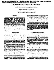
The algorithm is first demonstrated with a toy example in Figure 1. The data (10,000 samples) comes from a two-dimensional spherically symmetric Gaussian distribution. The two-class auxiliary data changes only in the vertical dimension, indicating that only the vertical dimension is relevant. The algorithm learns to model only the relevant dimension.
O O O O O O O O O O O O
O
O
Fig. 1. A demonstration of the MAP algorithm. The probability density function of the data is shown in shades of gray and the cluster centers with circles. The conditional density of one of the two auxiliary classes is shown in the inset. (Here σ = 0.4)
As far as we know there do not exist alternative methods for precisely the same task, partitioning the primary data space to clusters that are homogeneous in terms of the auxiliary data. We have earlier compared the older mutual information maximizing variant (section 5.1) with two clustering methods: the plain mixture of Gaussians and MDA2 [8, 9], a mixture model for the joint distribution of primary and auxiliary data. For gene expression data our algorithm outperformed the alternatives [2]. Here we will add the new variant (section 5.2) to the comparison. A random half of the Landsat satellite data set from the UCI Machine Learning Repository (36 dimensions, six classes, and 6435 samples) was partitioned into 2–10 clusters, using the six-fold class indicator as the auxiliary data. For each number of clusters, solutions were computed for 30 values of the smoothing parameter σ, ranging from two to 100 on the logarithmic scale. All the prior parameters n0i were set to unity. The models were evaluated by computing the log-posterior probability (7) of the left-out data. The log-posterior probabilities of the validation set are presented in Figure 2. For all numbers of clusters the new algorithm performed better, having a larger edge at smaller numbers of clusters. Surprisingly, in constrast to earlier experiments with other data sets, for this data set the alternative clustering methods seem to outperform the older variant of discriminative clustering.
5 clusters
6 clusters
7 clusters
-2000
-2000
-2000
-3000
-3000
-3000
-4000
-4000
-4000
-5000
-5000
-5000
2.
5.
10.0
20.
50.
2.
5.
8 clusters
10.0
20.
50.
2.
-2000
-2000
-3000
-3000
-3000
-4000
-4000
-4000
-5000
-5000
-5000
5.
10.0
20.
50.
2.
5.
10.0
20.
10.0
20.
50.
10 clusters
-2000
2.
5.
9 clusters
50.
2.
5.
10.0
20.
50.
Fig. 2. The performance of the conjugate-gradient MAP algorithm (solid line) compared to the older discriminative clustering algorithm (dashed line), plain mixture of Gaussians (dotted line) and MDA2, a mixture model for the joint distribution of primary and auxiliary data (dash-dotted line). Sets of clusters were computed with each method with several values of the smoothing parameter σ, and the posterior logprobability (7) of the validation data is shown for a hard assignment of each sample to exactly one cluster. Results measured with empirical mutual information (not shown) are qualitatively similar. The smallest visible value corresponds to assigning all samples to the same cluster
For 4–7 clusters, the models were compared by ten-fold cross-validation. The best value for σ was chosen with validation data, in preliminary tests. The new model was significantly better for all cluster numbers (paired t test, p< 0.001).
7
Conclusions
In summary, we have applied the learning metrics principle to clustering, and coined the approach discriminative clustering. It was shown that discriminative clustering is asymptotically, in the limit of a large number of clusters, equivalent to clustering in Fisher metrics, with the additional constraint that the clusters are (Euclidean) Voronoi regions in the primary data space. In the earlier work [1] Fisher metrics were derived from explicit conditional density estimators for clustering with Self-Organizing Maps; discriminative clustering has the advantage that the (arbitrary) density estimator is not required.
We have derived a finite-data discriminative clustering method that maximizes the posterior probability of the cluster centroids. There exist related methods for infinite data, proposed by us and others, derived by maximizing the mutual information [2, 10, 11]. For discrete primary data there exist also finite-data generative models [12, 13]; the main difference in our methods is the ability to derive a metric to continuous primary data spaces. Finally, we have shown that the cost function is equivalent to the Bayes factor of a contingency table with the marginal distribution of the auxiliary data fixed. The Bayes factor is the odds of the data likelihood given the hypothesis that the rows and columns are independent, vs. the alternative hypothesis of dependency. Hence, discriminative clustering can be interpreted to find a set of clusters that maximize the statistical dependency with the auxiliary data. Acknowledgments This work was supported by the Academy of Finland, in part by the grants 50061 and 52123.
References 1. Kaski, S., Sinkkonen, J., Peltonen, J.: Bankruptcy analysis with self-organizing maps in learning metrics. IEEE Trans. Neural Networks 12 (2001) 936–947 2. Sinkkonen, J., Kaski, S.: Clustering based on conditional distributions in an auxiliary space. Neural Computation 14 (2002) 217–239 3. Kullback, S.: Information Theory and Statistics. Wiley, New York (1959) 4. Agresti, A.: A survey of exact inference for contingency tables. Statistical Science 7 (1992) 131–153 5. Fisher, R. A.: On the interpretation of χ2 from the contingency tables, and the calculation of p. J. Royal Stat. Soc. 85 (1922) 87–94 6. Freeman, G. H., Halton, J. H.: Note on an exact treatment of contingency, goodness of fit and other problems of significance. Biometrika 38 (1951) 141–149 7. Good, I. J.: On the application of symmetric Dirichlet distributions and their mixtures to contingency tables. Annals of Statistics 4 (1976) 1159–1189 8. Hastie, T., Tibshirani, R., Buja, A.: Flexible discriminant and mixture models. In Kay, J. Titterington, D. (eds): Neural Networks and Statistics. Oxford University Press (1995) 9. Miller, D. J., Uyar, H. S.: A mixture of experts classifier with learning based on both labelled and unlabelled data. In Mozer, M., Jordan, M., Petsche, T. (eds): Advances in Neural Information Processing Systems 9. MIT Press, Cambridge, MA (1997) 571–577 10. Becker, S.: Mutual information maximization: models of cortical self-organization. Network: Computation in Neural Systems 7 (1996) 7–31 11. Tishby, N., Pereira, F. C., Bialek, W.: The information bottleneck method. In: 37th Annual Allerton Conference on Communication, Control, and Computing. Urbana, Illinois (1999) 12. Hofmann, T., Puzicha, J., Jordan, M. I.: Learning from dyadic data. In: Kearns, M. S., Solla, S. A., Cohn, D. A. (eds): Advances in Neural Information Processing Systems 11. Morgan Kaufmann Publishers, San Mateo, CA (1998) 466–472
13. Hofmann, T.: Unsupervised learning by probabilistic latent semantic analysis. Mach. Learning (2001) 177–196
A
Connection of MAP Estimation to Maximization of Mutual Information
The Stirling approximation log Γ(s + 1) = s log s − s + O(log s) applied to (8) yields X X Sj log(Sj + Nc − 1) sji log sji − log p({m}|D(c) , D(x) ) = j
ij
− (Nc − 1)
X
log(Sj + Nc − 1) + O(Nc k(log S + 1)) .
j
� The zeroth-order Taylor expansion log(S + n) = log S + O Sn gives after rearrangements, for Sj > 1, X X Sj log Sj + O(Nc k(log S + 1)) . sji log sji − log p({m}|D(c) , D(x) ) = j
ij
Division by S then gives (9).
B
Gradient of the MAP Cost Function
Denote for brevity tji = nji + n0i and Tj = respect to mj is
P
i tji .
The gradient of (15) with
X X ∂ X ∂ ∂ log p({m}|D(c) , D(x) ) = yl (x)Ψ(tli ) − yl (x)Ψ(Tl ) ∂mj ∂mj ∂mj il c(x)=i
x,l
X ∂ = yl (x)[Ψ(tl,c(x) ) − Ψ(Tl )] . ∂mj x,l
It is straightforward to show that for normalized Gaussian membership functions ∂ 1 yl (x) = 2 (x − mj )(δlj − yl (x))yj (x) . ∂mj σ Substituting this to the gradient gives X ∂ log p({m}|D(c) , D(x) ) = σ2 (x−mj )(δlj −yl (x))yj (x)[Ψ(tl,c(x) )−Ψ(Tl)] . ∂mj x,l
(17)
The final form (16) for the gradient results from applying the identity X X (δlj − yl )yj Ll = yl yj (Lj − Ll ) , l
to (17).
l