Jun 15, 2010 - We describe a novel translation modeling framework based on .... lation modeling, we take inspiration from recent advances in statistical parsing. Parsing .... tasks using standard data sets, as well as the NIST Urdu-to-English.
Discriminative Feature-Rich Modeling for Syntax-Based Machine Translation Kevin Gimpel Language Technologies Institute School of Computer Science Carnegie Mellon University 5000 Forbes Avenue Pittsburgh, PA 15213, USA
June 15, 2010
Dissertation Committee: Noah A. Smith (chair), Carnegie Mellon University Jaime G. Carbonell, Carnegie Mellon University Stephan Vogel, Carnegie Mellon University Eric P. Xing, Carnegie Mellon University David Chiang, University of Southern California, Information Sciences Institute
Abstract State-of-the-art statistical machine translation systems are most frequently built on phrasebased (Koehn et al., 2003) or hierarchical translation models (Chiang, 2005). In addition, a wide variety of models exploiting syntactic annotation on either the source or target side (or both) have recently been developed and also give state-of-the-art performance (Galley et al., 2006; Zollmann and Venugopal, 2006; Huang et al., 2006; Shen et al., 2008; Liu et al., 2009; DeNeefe and Knight, 2009). It is unclear which of these approaches works best in general or how we can combine their virtues in a single system. Furthermore, the community’s emphasis on inventing diverse structural approaches to translation has shifted the focus away from feature-rich modeling as it has been applied to other problems in NLP. For example, adding rich non-local features that violate structural independence assumptions of traditional models has led to state-of-the-art performance in statistical parsing (Huang, 2008b; Martins et al., 2009), but long-distance features have received scant attention from machine translation researchers. In this thesis, we explore feature-rich models for machine translation that make use of nonlocal features and bring together features from multiple formalisms into a single model. To achieve this goal, we make contributions to modeling, inference, and training for statistical machine translation. We describe a novel translation modeling framework based on quasi-synchronous grammar (QG; Smith and Eisner, 2006b). QG is flexible enough to generalize any synchronous formalism, providing an ideal testbed for comparison and integration of feature sets. Since QG does not require the source and target trees to be isomorphic, it permits simulation of the majority of approaches to machine translation in the literature. The modeling innovations we propose rely on efficient algorithms for approximate inference. The models we consider—log-linear models over lattices and hypergraphs—are not natural to encode using the machinery of graphical models, so we instead propose algorithms that extend or exploit well-understood dynamic programming algorithms for these models. We describe a technique called cube summing (Gimpel and Smith, 2009a) that provides a way to extend dynamic programming algorithms to compute expectations for non-local features. To this end, we also propose importance sampling algorithms as an alternative with better-understood theoretical properties. For training translation models, we present two novel objective functions that can be optimized with gradient methods: softmax-margin and the Jensen risk bound (JRB) (Gimpel and Smith, 2010a). Unlike the widely-used technique known as minimum error rate training (MERT; Och, 2003), our objectives can handle hidden variables, support regularization, and scale well to large numbers of features. Softmax-margin and JRB training are also more efficient and easier to implement than minimizing risk (Li and Eisner, 2009). We integrate these developments in a novel machine translation system that we use to conduct controlled experiments in comparing and combining feature sets from many different translation models. Preliminary results have been obtained for a small-scale German-English translation task and show promising trends for combining features from phrase-based and dependency-based syntactic translation models using approximate inference (Gimpel and Smith, 2009b). i
Contents 1
Introduction
2
Modeling 2.1 A Feature-Rich Translation Model . . . . . . . . . 2.2 Quasi-Synchronous Grammar . . . . . . . . . . . . 2.3 Decoding . . . . . . . . . . . . . . . . . . . . . . . . 2.3.1 Translation as Monolingual Lattice Parsing 2.3.2 Source-Side Coverage Features . . . . . . . 2.4 Training . . . . . . . . . . . . . . . . . . . . . . . . 2.5 Experiments . . . . . . . . . . . . . . . . . . . . . . 2.5.1 Results . . . . . . . . . . . . . . . . . . . . . 2.6 Proposed Work . . . . . . . . . . . . . . . . . . . .
3
4
5
1
. . . . . . . . .
. . . . . . . . .
. . . . . . . . .
. . . . . . . . .
. . . . . . . . .
. . . . . . . . .
. . . . . . . . .
. . . . . . . . .
. . . . . . . . .
. . . . . . . . .
. . . . . . . . .
. . . . . . . . .
. . . . . . . . .
4 5 6 6 7 7 8 9 10 11
Inference 3.1 Approximate Dynamic Programming with Non-Local Features 3.1.1 Dynamic Programming, Semirings, and Feature Locality 3.1.2 Cube Decoding . . . . . . . . . . . . . . . . . . . . . . . . 3.1.3 Cube Summing . . . . . . . . . . . . . . . . . . . . . . . . 3.1.4 Experiments . . . . . . . . . . . . . . . . . . . . . . . . . . 3.2 Proposed Work . . . . . . . . . . . . . . . . . . . . . . . . . . . . 3.2.1 Importance Sampling . . . . . . . . . . . . . . . . . . . .
. . . . . . .
. . . . . . .
. . . . . . .
. . . . . . .
. . . . . . .
. . . . . . .
. . . . . . .
. . . . . . .
. . . . . . .
. . . . . . .
. . . . . . .
. . . . . . .
13 14 14 16 18 19 20 21
Learning 4.1 Training Methods for Structured Linear Models 4.2 Softmax-Margin . . . . . . . . . . . . . . . . . . . 4.2.1 Relation to Other Objectives . . . . . . . . 4.2.2 Hidden Variables . . . . . . . . . . . . . . 4.3 Jensen Risk Bound . . . . . . . . . . . . . . . . . 4.4 Experiments and Discussion . . . . . . . . . . . . 4.5 Proposed Work . . . . . . . . . . . . . . . . . . .
. . . . . . .
. . . . . . .
. . . . . . .
. . . . . . .
. . . . . . .
. . . . . . .
. . . . . . .
. . . . . . .
. . . . . . .
. . . . . . .
. . . . . . .
. . . . . . .
25 25 27 27 28 28 29 30
Summary of Proposed Work
. . . . . . .
. . . . . . . . .
. . . . . . .
. . . . . . . . .
. . . . . . .
. . . . . . . . .
. . . . . . .
. . . . . . . . .
. . . . . . .
. . . . . . . . .
. . . . . . .
. . . . . . . . .
. . . . . . .
. . . . . . . . .
. . . . . . .
. . . . . . .
31
ii
Chapter 1
Introduction As machine translation (MT) has improved over the past decade, many diverse and successful approaches have emerged. Most recently, a flurry of activity in syntactic translation modeling has produced a large number of novel translation systems, many of which achieve impressive performance improvements over strong baselines (Yamada and Knight, 2001; Chiang, 2005; Galley et al., 2006; Zollmann and Venugopal, 2006; Huang et al., 2006; Shen et al., 2008; Liu et al., 2009; DeNeefe and Knight, 2009). Yet these approaches are diverse, using different grammatical formalisms and features, and it is unclear how to compare them or to combine their strengths into a single system. Some use a parse tree for the source sentence (“tree-to-string”), others produce a parse when generating the target sentence (“string-to-tree”), and others combine both (“tree-to-tree”). Each contains a unique set of features used to score a translation and constraints to make decoding tractable, both of which arise from the particular choice of grammatical formalism and form of the grammar rules. Different choices reflect different independence assumptions and require different decoding algorithms. As a result, syntactic features are rarely shared across models; algorithmic complexity and hard constraints in each model deter this possibility. In considering how to take advantage of the growing number of disparate approaches to translation modeling, we take inspiration from recent advances in statistical parsing. Parsing performance has improved through (1) the use of non-local features (Huang, 2008b; Martins et al., 2009), which violate structural independence assumptions, and (2) combination of features from multiple formalisms—namely, phrase-structure parsing and dependency parsing—in a single model (Carreras et al., 2008). In this thesis, we explore feature-rich models that seek to do the same for machine translation. The recent success of system combination in MT evaluations has shown how much there can be gained by combining diverse approaches to translation (NIST, 2009). Our approach differs from system combination by allowing the weights for individual features of each system to be learned jointly. We also wish to add many non-local features that are not present in any other system, and for this we need a framework that supports feature-rich inference and learning. Therefore, to achieve our goal, we make contributions to modeling, inference, and training for statistical machine translation systems. Modeling (§2): We describe a novel translation modeling framework based on a formalism called quasi-synchronous grammar (QG; Smith and Eisner, 2006b). QG is flexible enough to generalize any synchronous formalism, providing an ideal testbed for comparison and integration of feature sets. QG also allows relaxing many of the hard constraints of previous models, for example the constraint that derivations of bilingual grammars must be synchronous. Departures from synchrony are penalized softly using features, allowing the model to learn which non-isomorphic constructs are helpful and which can be dangerous for a particular language pair. We plan to 1
2
CHAPTER 1. INTRODUCTION
use the flexibility of QG to investigate empirically how individual feature sets compare in a controlled modeling and decoding framework, as well as to measure the effects of combination. In initial exploration, we have combined features from phrase-based systems with features of sourceand target-side dependency trees (Gimpel and Smith, 2009b). We propose to incorporate features from hierarchical phrase models (Chiang, 2005) and synchronous dependency grammars (Quirk et al., 2005; Shen et al., 2008), as well as novel non-local features, such as high-order class-based language models and language models with gaps. Inference (§3): The modeling innovations we propose rely on efficient algorithms for approximate inference. The models of greatest interest for machine translation are log-linear models over paths and hyperpaths, such as weighted finite-state machines and weighted context-free grammars. Such models are not natural to encode using the standard language of graphical models; attempts to do so result in many deterministic potentials, causing problems for standard approximate inference algorithms such as Gibbs sampling and belief propagation. We instead turn our attention to algorithms that extend or exploit well-understood dynamic programming algorithms. We describe a technique called cube summing (Gimpel and Smith, 2009a) that provides a way to extend dynamic programming algorithms for summing—like the forward and inside algorithms—with non-local features. Inspired by cube pruning (Chiang, 2007; Huang and Chiang, 2007), which augments decoding algorithms with non-local features, cube summing can be used for computing non-local feature expectations for discriminative training. To this end, we also propose importance sampling algorithms as an alternative with better-understood theoretical properties. We propose to perform an empirical comparison of these and other approximate inference techniques to determine which work best for the particular non-local features present in our models. We also propose to address inference at decoding time through the use of cube pruning coupled with a coarse-to-fine approach with several stages of models, using subsets of feature categories—phrase features, hierarchical phrase features, etc.—for the sequence of models of increasing complexity. Learning (§4): We contribute novel objective functions for training the weights of machine translation models. The standard solution has been minimum error rate training (MERT; Och, 2003), which seeks to directly minimize error of a training set. Relying on coordinate ascent and lacking regularization, MERT fails to scale well to large numbers of features and has frequently been observed to overfit. Furthermore, like large-margin training methods, MERT does not have a principled way to handle hidden variables. To address these deficiencies, we present two novel objective functions for training translation models: softmax-margin and the Jensen risk bound (JRB) (Gimpel and Smith, 2010a). Both can be optimized with standard gradient methods and combine a probabilistic interpretation with the ability to use a task-specific cost function. They support regularization, can handle hidden variables, and scale well to large numbers of features. Both are bounds on risk (Smith and Eisner, 2006a; Li and Eisner, 2009) but are more efficient to train and easier to implement; softmax-margin is a loose convex bound and JRB is a tighter bound that is non-convex. We propose to compare softmax-margin and JRB training with several commonly-used training methods for structured prediction, both for standard phrase-based models (Koehn et al., 2007) as well as our feature-rich translation models. We integrate these developments in a novel machine translation system and plan to conduct controlled experiments in comparing and combining feature sets from many different translation models (§5). Preliminary results have been obtained for a small-scale German-English translation task using this framework, and show promising trends for combining features from phrase-based and dependency-based syntactic translation models using approximate inference (Gimpel and
3 Smith, 2009b). We plan to conduct additional experiments for large-scale German-to-English and Chinese-to-English translation tasks using standard data sets, as well as the NIST Urdu-to-English task as a contrastive small-data scenario. We will compare with state-of-the-art phrase-based and hierarchical MT systems as baselines, using four automatic metrics: BLEU (Papineni et al., 2001), METEOR (Banerjee and Lavie, 2005), TER (Snover et al., 2006), and TER-Plus (Snover et al., 2009). While the primary goal of this thesis is to study feature-rich models for machine translation both analytically and experimentally, we also have a secondary goal: to build stronger connections between machine translation and machine learning. Due to the immensity of the modeling and engineering challenges in MT, there has been only limited interest from researchers in using inference and learning algorithms whose theoretical properties have been analyzed. The popularity of the MERT algorithm is a prime example of this. Despite work showing other methods to perform better (Smith and Eisner, 2006a; Chiang et al., 2009; Li and Eisner, 2009), MERT remains a fixture in the MT community and is used in the vast majority of publications and submissions to shared translation tasks. In this thesis, we offer additional options for inference and learning to the MT community that have theoretical motivation, and plan to conduct extensive experiments to determine when they can be useful in practice. We also intend to describe these techniques in sufficient generality so that they can be applied to other problems in natural language processing and structured prediction. This dissertation will demonstrate that combining structural and non-local features from different translation formalisms in a discriminative learning framework can significantly improve translation quality. The methods we develop to achieve this goal will be described in sufficient generality to be applicable to other structured prediction tasks in natural language processing and machine learning.
Chapter 2
Modeling The machine translation community has seen a surge of recent innovations in translation modeling. Beginning with the success of phrase-based translation models (Koehn et al., 2003), a trend arose of performing translation by modeling larger and increasingly complex structural units. Current research efforts are actively exploring approaches to incorporating syntax into translation models. The approaches can be broadly differentiated by which language—source, target, or both—receives syntactic analysis. If the source side is parsed and translation proceeds by producing a target-side string, the approach is tree-to-string or syntax-directed translation (Huang et al., 2006). If the source sentence is not parsed by a monolingual parser and instead translation proceeds by building a target tree from a source string, the approach is string-to-tree (Galley et al., 2006; Zollmann and Venugopal, 2006; Shen et al., 2008). The final category, tree-to-tree, translates a parsed source sentence into a target sentence with parse tree (Liu et al., 2009; Chiang, 2010). These approaches are often described in terms of “rules” and “features”; the choice of formalism determines the grammar rules and relative frequency estimates are typically the only features associated with each rule. Decoding algorithms frequently assume that the input is transduced to the output by following a sequence of rules. Hence, it may be difficult to imagine two different formalisms operating in tandem to generate a translation; their rules would likely conflict. We will instead think solely in terms of the features associated with each rule in each formalism, and allow overlapping features from multiple formalisms to score a translation wherever their rules would “fire” (i.e., be invoked) during the process of translation. Since the full set of active features would often violate the structural independence assumptions of a decoder based on dynamic programming, we need a way to deal with non-local features. In this chapter, we define a globally-normalized log-linear translation model that can be used to encode any features on source and target sentences, dependency trees, and alignments. The trees are optional and can be easily removed, allowing simulation of tree-to-string, string-to-tree, tree-to-tree, and phrase-based models, among others. The core of the approach is a novel decoder based on lattice parsing with quasi-synchronous grammar (QG; Smith and Eisner, 2006b), a flexible formalism that does not require source and target trees to be isomorphic. We exploit generic approximate inference techniques to incorporate arbitrary non-local features in the dynamic programming algorithms (Chiang, 2007; Gimpel and Smith, 2009a). These techniques are discussed in more detail in §3.
4
2.1. A FEATURE-RICH TRANSLATION MODEL Σ, T Trans : Σ ∪ {NULL} → 2T s = hs0 , . . . , sn i ∈ Σn t = ht1 , . . . , tm i ∈ Tm τs : {1, . . . , n} → {0, . . . , n} τt : {1, . . . , m} → {0, . . . , m} a : {1, . . . , m} → 2{1,...,n} θ f
5
source and target language vocabularies, respectively function mapping each source word to target words to which it may translate source language sentence (s0 is the NULL word) target language sentence, translation of s dependency tree of s, where τs (i) is the index of the parent of si (0 is the root, $) dependency tree of t, where τt (i) is the index of the parent of ti (0 is the root, $) alignments from words in t to words in s; ∅ denotes alignment to NULL parameters of the model feature vector
Table 2.1: Key notation.
2.1
A Feature-Rich Translation Model
Given a sentence s and its parse tree τs , we formulate the translation problem as finding the target sentence t∗ (along with its parse tree τt∗ and alignment a∗ to the source tree) such that ht∗ , τt∗ , a∗ i = argmax p(t, τt , a | s, τs )
(2.1)
ht,τt ,ai
In order to include overlapping features and permit hidden variables during training, we use a single globally-normalized conditional log-linear model. That is, exp{θ > f (s, τs , a, t, τt )} > 0 0 0 a0 ,t0 ,τ 0 exp{θ f (s, τs , a , t , τt )}
p(t, τt , a | s, τs ) = P
(2.2)
t
where the f are arbitrary feature functions and the θ are feature weights. If one or both parse trees or the word alignments are unavailable, they can be ignored or marginalized out as hidden variables. Table 2.1 summarizes our notation. In structured log-linear models, the feasibility of inference depends upon the choice of feature functions f . Typically these feature functions are chosen to factor into local parts of the overall structure. Standard features for machine translation include lexical translation features (often in the form of word-to-word or phrase-to-phrase probabilities), N -gram language models, word and phrase penalties, and features to model reordering such as distortion and lexicalized reordering models (Koehn et al., 2007). There have also been many features proposed that consider source- and target-language syntax during translation. Syntax-based MT systems often use features on grammar rules, frequently maximum likelihood estimates of conditional probabilities in a probabilistic grammar, but other syntactic features are possible. For example, Quirk et al. (2005) use features involving phrases and source-side dependency trees and Mi et al. (2008) use features from a forest of parses of the source sentence. There is also substantial work in the use of target-side syntax (Galley et al., 2006; Marcu et al., 2006; Zollmann and Venugopal, 2006; Shen et al., 2008). We turn next to the “backbone” model for our decoder; the formalism and the properties of its decoding algorithm will inspire two additional sets of features.
6
CHAPTER 2. MODELING
2.2
Quasi-Synchronous Grammar
A quasi-synchronous dependency grammar (QDG; Smith and Eisner, 2006b) specifies a conditional model p(t, τt , a | s, τs ). Given a source sentence s and its parse τs , a QDG induces a probabilistic monolingual dependency grammar over sentences “inspired” by the source sentence and tree. We denote this grammar by Gs,τs ; its (weighted) language is the set of translations of s. Each word generated by Gs,τs is annotated with a “sense,” which consists of zero or more words from s. The senses imply an alignment (a) between words in t and words in s, or equivalently, between nodes in τt and nodes in τs .1 In principle, any portion of τt may align to any portion of τs , but in practice we often make restrictions on the alignments to simplify computation. Smith and Eisner, for example, restricted |a(j)| for all words tj to be at most one, so that each target word aligned to at most one source word, which we also do here.2 Which translations are possible depends heavily on the configurations that the QDG permits. Formally, for a parent-child pair htτt (j) , tj i in τt , we consider the relationship between a(τt (j)) and a(j), the source-side words to which tτt (j) and tj align. If, for example, we require that, for all j, a(τt (j)) = τs (a(j)) or a(j) = 0, and that the root of τt must align to the root of τs or to NULL , then strict isomorphism must hold between τs and τt , and we have implemented a synchronous context-free dependency grammar (Alshawi et al., 2000; Ding and Palmer, 2005). Smith and Eisner (2006b) grouped all possible configurations into eight classes and explored the effects of permitting different sets of classes in word alignment. (“a(τt (j)) = τs (a(j))” corresponds to their “parent-child” configuration; see Fig. 3 in Smith and Eisner (2006b) for illustrations of the rest.) Note that the QDG instantiates the model in Eq. 2.2. The syntactic, lexical translation, and distortion features can be easily incorporated into the QDG while respecting the independence assumptions implied by the configuration features. Phrase pair and language model features are non-local, or involve parts of the structure that, from the QDG’s perspective, are conditionally independent given intervening material. Note that “non-locality” is relative to a choice of formalism; in §2.1 we did not commit to any formalism, so it is only now that we can describe phrase and N -gram features as “non-local.”
2.3
Decoding
Given a sentence s and its parse τs , at decoding time we seek the target sentence t∗ , the target tree τt∗ , and the alignments a∗ that are most probable: ht∗ , τt∗ , a∗ i = argmax θ > f (s, τs , a, t, τt )
(2.3)
ht,τt ,ai
For a QDG model, the decoding problem equates to finding the most probable derivation under the source-sentence-specific grammar Gs,τs . We solve this by lattice parsing, assuming that an upper bound on m (the length of t) is known. The advantage offered by this approach (like most other grammar-based translation approaches) is that decoding becomes dynamic programming (DP), a technique that is both widely understood in NLP and for which efficient, generic techniques exist. 1
We note that while this equivalence exists when using dependency grammars, it does not hold for phrase structure grammars. 2 I.e., from here on, a : {1, . . . , m} → {0, . . . , n} where 0 denotes alignment to NULL.
could you translate it ? 2.3. DECODING
Source:
7
$ konnten sie es übersetzen ?
Reference:
could you translate it ?
$ k
Decoder output:
$
konnten:could
konnten:could
es:it
?:?
?:?
übersetzen: translate
übersetzen: translate
sie:you
sie:you
konnten:could
konnten:couldn konnten:might
es:it
sie:you
übersetzen: translated
übersetzen: translated
sie:let
?:?
es:it
es:it
es:it
sie:them
konnten:could
NULL:to
...
...
übersetzen: translate
...
...
...
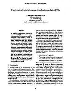
Figure 2.1: Decoding as lattice parsing, with the highest-scoring translation denoted by black lattice arcs (others are grayed out) and thicker blue arcs forming a dependency tree over them.
Source:
$ konnten sie es übersetzen ?
Reference:
2.3.1
could you translate it ?
Translation as Monolingual Lattice Parsing
output: WeDecoder decode by performing lattice parsing on a lattice encoding the set of possible translations. The lattice is a weighted “sausage” lattice that permits sentences up to some maximum length `, which is derived from the source sentence length.3 For every position between consecutive states j − 1 and j (where 0 < j ≤ `), and for every word si in s (including the NULL word s0 ), and for es:it t and i. The weight?:? konnten:could konnten:could $ word every t ∈ Trans(si ), we instantiate an arc annotated with of such an > übersetzen: arc is exp{θ f }, where f is the sum of feature functions that fire when si translates as t in target sie:you sie:you konnten:could position j (e.g., lexical translation and distortion features). Given the lattice andtranslate Gs,τs , lattice übersetzen: parsing iskonnten:couldn a straightforward generalization of standard context-free dependency parsing dynamic sie:you es:it translated programming algorithms (Eisner, 1997). konnten:might es:itfrom an sie:let ?:? with dependency tree Figure 2.1 shows an example with a German source sentence übersetzen: konnten:could automatic parser, and a lattice representing possible translations. In each es:it an English reference, sie:them translate bundle, the arcs are listed in decreasing order according to weight and for clarity only the first ... ... ... ... five are shown. The output of the decoder consists of lattice arcs selected at each position and a dependency tree over them. In this case, the output string equals the reference translation and the alignment and dependency tree are correct. 2.3.2
übe tra
übe tra
NU
Source-Side Coverage Features
Most MT decoders enforce a notion of “coverage” of the source sentence during translation: all parts of s should be aligned to some part of t (alignment to NULL incurs an explicit cost). Phrasebased systems such as Moses (Koehn et al., 2007) explicitly search for the highest-scoring string in which all source words are translated. Systems based on synchronous grammars proceed by parsing the source sentence with the synchronous grammar, ensuring that every phrase and word has an analogue in τt (or a deliberate choice is made by the decoder to translate it to NULL). In such systems, we do not need to use features to implement source-side coverage, as it is assumed
$ 3
konnten:could
konnten:could
es:it
Let the states be numbered 0 to `; states from bρ`c to ` are final states (for some ρ ∈ (0, 1)).
?:?
übersetzen: translate
sie:you
sie:you
konnten:could
konnten:couldn konnten:might
es:it
sie:you
übersetzen: translated
sie:let
?:?
es:it
es:it
sie:them
konnten:could
...
...
übersetzen: translate
...
...
übe tra
übe tra
NU
8
CHAPTER 2. MODELING
as a hard constraint always respected by the decoder. Our QDG decoder has no way to enforce coverage; it does not track any kind of state in τs apart from a single recently aligned word. Our solution is to introduce a set of coverage features which consist of the following: • A counter for the number of times each source word is covered. • Features that fire once when a source word is covered the zth time (z ∈ {2, 3, 4}) and fire again all subsequent times it is covered. • A counter of uncovered source words. Of these, only the first is local. The lattice QDG parsing decoder incorporates many of the features we have discussed, but not all of them. Phrase lexicon features, language model features, and most coverage features are non-local with respect to our QDG. Recently Chiang (2007) introduced “cube pruning” as an approximate decoding method that extends a DP decoder with the ability to incorporate features that break the independence assumptions DP exploits. Techniques like cube pruning can be used to include the non-local features in our decoder. We actually use “cube decoding,” a less approximate but more expensive method that is more closely related to the approximate inference method we use for training, discussed in §2.4.
2.4
Training
Training requires us to learn values for the parameters θ in Eq. 2.2. Given D training examples (i) (i) of the form ht(i) , τt , s(i) , τs i, for i = 1, ..., D, maximum likelihood estimation for this model consists of solving the following:4 max LL(θ) = max θ
θ
D X
(i)
log p(t
(i) , τt
(i)
|s
(i) , τs )
i=1
= max θ
D X i=1
> f (s(i) , τ (i) , a, t(i) , τ (i) )} s t P (i) > (i) t,τt ,a exp{θ f (s , τs , a, t, τt )}
P log
a exp{θ
(2.4) Note that the alignments are treated as a hidden variable to be marginalized out.5 Training is typically performed using variations of gradient ascent. This requires us to calculate the function’s gradient with respect to θ. Computing the numerator in Eq. 2.4 involves summing over all possible alignments, which can be done efficiently with a dynamic program (Gimpel and Smith, 2009b). Computing the denominator in Eq. 2.4 requires summing over all word sequences and dependency trees for the target language sentence and all word alignments between the sentences. With a maximum length imposed, this is tractable using the “inside” version of the maximizing DP algorithm of Sec. 2.3, but it is prohibitively expensive. We therefore optimize pseudo-likelihood instead, making the following approximation (Besag, 1975): p(t, τt | s, τs ) ≈ p(t | τt , s, τs ) × p(τt | t, s, τs ) Plugging this into Eq. 2.4, we arrive at max PL(θ) = max θ
θ
D X i=1
log
�X a
(i)
p(t , a |
� X �X � D (i) (i) (i) (i) + log p(τt , a | t , s , τs )
(i) (i) τt , s(i) , τs )
i=1
a
(2.5) 4
In practice, we regularize by including a term −ckθk22 . Alignments could be supplied by automatic word alignment algorithms. We chose to leave them hidden so that we could make the best use of our parsed training data when hard configuration constraints are imposed (as in the experiments of Table 2.3), since it is not always possible to reconcile automatic word alignments with automatic parses. 5
2.5. EXPERIMENTS
9
The two parenthesized terms in Eq. 2.5 each have their own numerators and denominators (not shown). The numerators are identical to each other and to that in Eq. 2.4. The denominators are much more manageable than in Eq. 2.4, never requiring summation over more than two structures at a time. We must sum over target word sequences and word alignments (with fixed τt ), and separately over target trees and word alignments (with fixed t). Dynamic programming algorithms for performing these summations are provided in Gimpel and Smith (2009b). To extend these dynamic programming algorithms with non-local features, we use a technique that we call cube summing, an approximate method that permits the use of non-local features for inside DP algorithms (Gimpel and Smith, 2009a). Cube summing is based on a slightly less greedy variation of cube pruning (Chiang, 2007) that maintains k-best lists of derivations for each DP chart item. Using the machinery of cube summing, it is straightforward to include the desired non-local features in the summations required for pseudolikelihood, as well as to compute their approximate gradients. In §3, we discuss cube summing in detail and describe alternatives that we propose for the thesis. We also present some additional experimental results. Our approach permits an alternative to minimum error-rate training (MERT; Och, 2003); it is discriminative but handles latent structure and regularization in more principled ways. The pseudolikelihood calculations for a sentence pair, taken together, are faster than decoding, making our training procedure faster than MERT. However, conditional likelihood and pseudolikelihood do not allow us to incorporate automatic MT evaluation metrics into training. In §4 we describe alternative learning objectives that address this issue, and still allow marginalizing out hidden variables as we do here.
2.5
Experiments
Our decoding framework allows us to perform many experiments with the same feature representation and inference algorithms. In the thesis, we intend to perform more rigorous experiments for multiple language pairs. We include here experiments for German-to-English translation with combining and comparing phrase-based and syntax-based features and examining how isomorphism constraints of synchronous formalisms affect translation output. We use the German-English portion of the Basic Travel Expression Corpus (BTEC). The corpus has approximately 100K sentence pairs. We filter sentences of length more than 15 words, which removes 6% of the data. We end up with a training set of 82,299 sentences, a development set of 934 sentences, and a test set of 500 sentences. We evaluate translation output using caseinsensitive BLEU (Papineni et al., 2001), as provided by NIST, and METEOR (Banerjee and Lavie, 2005), version 0.6, with Porter stemming and WordNet synonym matching. We will now discuss the features used in our experiments. To obtain lexical translation features, we use the Moses pipeline (Koehn et al., 2007): we perform word alignment using GIZA++ (Och and Ney, 2003), symmetrize the alignments using the “grow-diag-final-and” heuristic, and extract phrases up to length 3. We use 8 lexical translation features: {2, 3} target words × phrase conditional and “lexical smoothing” probabilities × two conditional directions. Bigram and trigam language model features are estimated using the SRI toolkit (Stolcke, 2002) with modified Kneser-Ney smoothing (Chen and Goodman, 1998). For our target-language syntactic features, we use features similar to lexicalized CFG events (Collins, 1999), specifically following the dependency model of Klein and Manning (2004). These include probabilities associated with individual attachments and child-generation valence probabilities. These probabilities are estimated on the training corpus parsed using the Stanford parser (Klein and Manning, 2003). The same probabilities are also included using 50 hard word classes derived from the parallel corpus using the GIZA++ mkcls utility. In total, there are 7 lexical and 7 word-class syntax features. For reordering, we use a single absolute distortion feature that returns |i − j| whenever a(j) = i and
10
CHAPTER 2. MODELING Phrase features: +
Syntactic Features: Target Syntax 0.3727 0.4458 0.4682 0.4971
Tree-to-tree 0.4424 0.5142
Table 2.2: Feature set comparison (BLEU scores are shown; METEOR scores were qualitatively similar).
i, j > 0.The tree-to-tree syntactic features in our model are binary features that fire for particular QG configurations. We use one feature for each of the configurations given by Smith and Eisner (2006b), adding 7 additional features that score configurations involving root words and NULLalignments more finely. We use the coverage features described in §2.3.2. In all, 46 feature weights are learned. We used the parallel data to estimate feature functions and the development set to train θ. We trained using three iterations of stochastic gradient ascent over the development data with a batch size of 1 and a fixed step size of 0.01.6 We used `2 regularization with a coefficient of 0.1. We used a 10-best list with cube summing during training and a 7-best list for cube decoding when decoding the test set. To obtain the translation lexicon (Trans) we first included the top three target words t ∈ T for each s ∈ Σ using p(s | t) × p(t | s) to score target words. For any training sentence hs, ti and tj for S which tj 6∈ ni=1 Trans(si ), we added tj to Trans(si ) for i = argmaxi0 ∈I p(si0 |tj ) × p(tj |si0 ), where I = {i : 0 ≤ i ≤ n ∧ |Trans(si )| < qi }. We used q0 = 10 and q>0 = 5, restricting |Trans(NULL)| ≤ 10 and |Trans(s)| ≤ 5 for any s ∈ Σ. This made 191 of the development sentences unreachable by the model, leaving 743 sentences for learning θ. It is not uncommon for syntax-based machine translation systems to encounter this situation, especially when maximizing likelihood (Blunsom et al., 2008). This highlights another drawback of using likelihood-based objectives for MT; we return to this issue and propose a solution in §4. During decoding, we generated lattices with all t ∈ Trans(si ) for 0 ≤ i ≤ n, for every position. Between each pair of consecutive states, we pruned edges that fell outside a beam of 70% of the sum of edge weights; edge weights use lexical translation, absolute distortion, and coverage features.
2.5.1
Results
Our first set of experiments compares feature sets commonly used in phrase- and syntax-based translation. The base model contains lexical translation features, the language model, the absolute distortion feature, and the coverage features. The results are shown in Table 2.2. The second row contains scores when adding in the eight phrase translation features. The second column shows scores when adding the 14 target syntax features, and the third column adds to them the 14 additional tree-to-tree features. We find large gains in BLEU by adding more features, and find that gains obtained through phrase features and syntactic features are partially additive, suggesting that these feature sets are making complementary contributions to translation quality. 6
Three iterations may seem like a small number; this was not chosen for runtime reasons, as it only took a couple hours to complete each training run, but rather for performance. We did not tune the number of iterations, but noticed in preliminary experiments that while feature weights for local features converged quickly, there was a different story for non-local features. The bias in their expectations as computed by cube summing caused their weights to continue to grow in magnitude as training proceeded. We return to this issue of bias in computing expectations of non-local features in §3.
2.6. PROPOSED WORK
11 QDG Configurations synchronous + nulls, root-any + child-parent, same node + sibling + grandparent/child + c-command + other
BLEU 0.4008 0.4108 0.4337 0.4881 0.5015 0.5156 0.5142
METEOR 0.6949 0.6931 0.6815 0.7216 0.7365 0.7441 0.7472
Table 2.3: QG configuration comparison. The name of each configuration, following Smith and Eisner (2006b), refers to the relationship between a(τt (j)) and a(j) in τs .
We next compare different constraints on isomorphism between the source and target dependency trees. To do this, we impose harsh penalties on some QDG configurations (§2.2) by fixing their feature weights to −1000. Hence they are permitted only when absolutely necessary in training and rarely in decoding.7 Each model uses all phrase and syntactic features; they differ only in the sets of configurations which have fixed negative weights. Table 2.3 shows experimental results. The base “synchronous” model permits parent-child (a(τt (j)) = τs (a(j))), any configuration where a(j) = 0, including both words being linked to NULL , and requires the root word in τt to be linked to the root word in τs or to NULL (5 of our 14 configurations). The second row allows any configuration involving NULL, including those where tj aligns to a non-NULL word in s and its parent aligns to NULL, and allows the root in τt to be linked to any word in τs . Each subsequent row adds additional configurations (i.e., trains its θ rather than fixing it to −1000). In general, we see large improvements as we permit more configurations, and the largest jump occurs when we add the “sibling” configuration (τs (a(τt (j))) = τs (a(j))). The BLEU score does not increase, however, when we permit all configurations in the final row of the table, and the METEOR score increases only slightly. While allowing certain categories of non-isomorphism clearly seems helpful, permitting arbitrary violations does not appear to be necessary for this dataset. Our findings show that phrase features and dependency syntax produce complementary improvements to translation quality, that tree-to-tree configurations are helpful for translation, and that substantial gains can be obtained by permitting certain types of non-isomorphism.
2.6
Proposed Work
We note that these results are not state-of-the-art on this dataset (on this task, Moses/MERT achieves 0.6838 BLEU and 0.8523 METEOR with maximum phrase length 3). We believe our results are currently at the level of a proof of concept. Nonetheless, we believe that with some engineering, we can improve our results substantially, in addition to the contributions of §3 and §4, which have not yet been integrated into this system. In particular, we believe that combining cube pruning with coarse-to-fine decoding will speed up the decoder significantly, allowing us to prune less during search and reach better translations (Charniak and Johnson, 2005; Petrov, 2009). In addition to the engineering required for our system to reach competitive performance, we plan to conduct extensive investigation into adding features. Some of the feature sets we plan to 7
In fact, the strictest “synchronous” model used the almost-forbidden configurations in 2% of test sentences; this behavior disappears as configurations are legalized.
12
CHAPTER 2. MODELING Features Lexical + language model + distortion + coverage + Phrases (Koehn et al., 2003) + Target dependency syntax (Klein and Manning, 2004) + Tree-to-tree configurations (Smith and Eisner, 2006b) + Hierarchical phrases (Chiang, 2005) + hSource dependency syntax → Target phrasei rules (Quirk et al., 2005) + hSource phrase → Target dependency syntaxi rules (Shen et al., 2008) + hSource dependency syntax → Target dependency syntaxi rules + Dependency language models (Shen et al., 2008) + Non-local high-order N -gram and class-based language models + Additional non-local features based on error analysis (see text)
BLEU 0.3727 0.4682 0.4971 0.5142
Table 2.4: Proposed features, along with BLEU scores from Table 2.2. We plan to conduct these experiments for multiple language pairs and translation tasks.
add are shown in Table 2.4, along with BLEU scores from Table 2.2 where applicable. The majority of features will be straightforward to add to our system, since we already include source- and target-side dependency trees. With the two categories of non-local features, we plan to experiment with novel features for MT. We plan to include non-local high-order N -gram language models trained on word classes obtained from distributional similarity clustering. We also plan to estimate high-order language models that contain gaps, of both fixed-length and variable-length, and use these as additional features. We also propose to include a category of non-local features that we derive based on error analysis. For example, for German-to-English translation, the main verb of the German sentence is often missing from the English translation due to long-distance reordering. Features that address these types of critical errors will be possible to include in our framework. Through these experiments, we seek to address the question of whether the many diverse feature sets of different approaches to MT can combine to give performance exceeding the stateof-the-art. We also hope to determine which feature sets contribute the most to translation quality and how the landscape changes for different language pairs.
Chapter 3
Inference Probabilistic NLP researchers frequently make independence assumptions to keep inference algorithms tractable. Doing so limits the features that are available to our models, requiring features to be structurally local. Yet many problems in NLP—machine translation, parsing, named-entity recognition, and others—have benefited from the addition of non-local features that break classical independence assumptions (Roth and Yih, 2004; Sutton and McCallum, 2004; Finkel et al., 2005; Chiang, 2007; Huang, 2008b; Smith and Eisner, 2008; Martins et al., 2009). Doing so requires algorithms for approximate inference. Consider a distribution p(y|x) over outputs y ∈ Y(x) given an observed input x. The two fundamental inference problems that we will consider are: • Computing the most probable output: yˆ = argmax p(y|x)
(3.1)
y∈Y(x)
• Computing the expectation of a function f (x, y) with respect to p(y|x): X Ep(·|x) [f (x, ·)] = p(y|x)f (x, y)
(3.2)
y∈Y(x)
In this thesis, we will focus on approximate inference algorithms that can be used for computing expectations (Eq. 3.2), rather than algorithms for decoding (Eq. 3.1). The machine translation community has devoted substantial effort toward developing efficient approximate decoding algorithms, e.g., cube pruning (Chiang, 2007; Huang and Chiang, 2007) and coarse-to-fine decoding (Petrov, 2009). For the remainder of this chapter, we focus our attention on approximate inference algorithms for computing expectations; these algorithms will be useful to compute feature expectations required for discriminative training methods to be introduced in §4. Our primary interest is in models commonly found in MT and NLP. Certain classes of these models cannot be easily described with the graphical vocabulary of traditional graphical models (Koller and Friedman, 2009). For example, consider a model over paths in a lattice. If we assign a random variable to each edge in the lattice, there will be complex interdependencies among the variables in the model. Hard constraints such as these, typically realized through deterministic clique potential functions, are known to cause slow mixing for Gibbs samplers. Furthermore, for models over paths and generally for models with recursive structure, NLP researchers have developed algorithms for exact inference that respect the constraints among output variables, often based on dynamic programming. We prefer to begin with these existing exact algorithms and extend or exploit them to develop approximate inference algorithms. We propose two such techniques. The first, cube summing, extends existing dynamic programming algorithms in order to 13
14
CHAPTER 3. INFERENCE
compute expectations for models with non-local features (§3.1.3). The second has the same goal, but is based on importance sampling and is asymptotically unbiased (§3.2.1).
3.1
Approximate Dynamic Programming with Non-Local Features
In this section, we present algorithms for approximate inference that extend existing dynamic programming algorithms for models common to NLP. We introduce cube summing, a technique that permits dynamic programming algorithms for summing over structures (like the forward and inside algorithms) to be extended with non-local features. It is inspired by cube pruning (Chiang, 2007; Huang and Chiang, 2007) in its computation of non-local features dynamically using scored k-best lists, but also maintains residual quantities used in calculating approximate marginals. When restricted to local features, cube summing reduces to a novel semiring that we call k-best+residual and that generalizes many of the semirings of Goodman (1999). When nonlocal features are included, cube summing does not reduce to any semiring, but is compatible with generic techniques for solving dynamic programming equations. We begin by discussing dynamic programming algorithms as semiring-weighted logic programs. It can be shown that semirings are too restrictive for certain applications of dynamic programming, notably approximate algorithms for inference in the presence of non-local features (Gimpel and Smith, 2009a). However, semirings are useful for understanding and succinctly describing dynamic programming algorithms, so we will use terminology and concepts from semirings to describe our algorithms. We will first present cube decoding (§3.1.2), which is a simplified version of cube pruning and which serves as a stepping stone to describe cube summing (§3.1.3).
3.1.1
Dynamic Programming, Semirings, and Feature Locality
Many algorithms in NLP involve dynamic programming (e.g., the Viterbi, forward-backward, probabilistic Earley’s, and minimum edit distance algorithms). Dynamic programming (DP) involves solving certain kinds of recursive equations with shared substructure and a topological ordering of the variables. Shieber et al. (1995) showed a connection between DP (specifically, as used in parsing) and logic programming, and Goodman (1999) augmented such logic programs with semiring weights, giving an algebraic explanation for the intuitive connections among classes of algorithms with the same logical structure. For example, in Goodman’s framework, the forward algorithm and the Viterbi algorithm are comprised of the same logic program with different semirings. For our purposes, a DP consists of a set of recursive equations over a set of indexed variables. To describe cube summing, we will make use of Shieber et al.’s logic programming view of dynamic programming. In this view, each variable in a dynamic program corresponds to the value of a “theorem,” the constants in the equations correspond to the values of “axioms,” and the DP defines quantities corresponding to weighted “proofs” of the goal theorem (e.g., finding the maximum-valued proof, or aggregating proof values). The value of a proof is a combination of the values of the axioms it starts with. Semirings define these values and define two operators over them, called “aggregation” and “combination.” Semirings Formally, a semiring is a tuple hA, ⊕, ⊗, 0, 1i, in which A is a set, ⊕ : A × A → A is the aggregation operation, ⊗ : A × A → A is the combination operation, 0 is the additive identity element (∀a ∈ A, a ⊕ 0 = a), and 1 is the multiplicative identity element (∀a ∈ A, a ⊗ 1 = a). A semiring requires ⊕ to be associative and commutative, and ⊗ to be associative and to distribute over ⊕. Finally, we require a ⊗ 0 = 0 ⊗ a = 0 for all a ∈ A.
3.1. APPROXIMATE DYNAMIC PROGRAMMING WITH NON-LOCAL FEATURES Semiring inside Viterbi Viterbi proof k-best proof
A R≥0 R≥0 R≥0 × L (R≥0 × L)≤k
Aggregation (⊕) u1 + u2 max(u1 , u2 ) hmax(u1 , u2 ), Uargmaxi∈{1,2} ui i max-k(u1 ∪ u2 )
Combination (⊗) u1 u2 u1 u2 hu1 u2 , U1 .U2 i max-k(u1 ? u2 )
0 0 0 h0, �i ∅
15 1 1 1 h1, �i {h1, �i}
Table 3.1: Commonly used semirings. An element in the Viterbi proof semiring is denoted hu1 , U1 i, where u1 is the probability of proof U1 . The max-k function returns a sorted list of the top-k proofs from a set and U1 .U2 denotes the string concatenation of U1 and U2 . The ? function performs a cross-product on two proof lists (Eq. 3.3).
Several examples are shown in Table 3.1, including the well-known inside and Viterbi semirings. The “Viterbi proof” semiring includes the probability of the most probable proof and the proof itself. Letting L ⊆ Σ∗ be the proof language on some symbol set Σ, this semiring is defined on the set R≥0 × L. The “k-best proof” semiring computes the values and proof strings of the k most-probable proofs for each theorem. The set is (R≥0 × L)≤k , i.e., sequences (up to length k) of sorted probability/proof pairs. The combination operator ⊗ requires a cross-product operator that pairs probabilities and proofs from two k-best lists. We call this ?, defined on two semiring values u = hhu1 , U1 i, ..., huk , Uk ii and v = hhv1 , V1 i, ..., hvk , Vk ii by: u ? v = {hui vj , Ui .Vj i | i, j ∈ {1, ..., k}}
(3.3)
Feature Locality Let X be the space of inputs to our logic program, i.e., x ∈ X is a set of axioms. Let L denote the proof language and let Y ⊆ L denote the set of proof strings that constitute full proofs, i.e., proofs of the special goal theorem. We assume an exponential probabilistic model such that Q hm (x,y) (3.4) p(y | x) ∝ M m=1 λm where each λm ≥ 0 is a parameter of the model and each hm is a feature function. As defined, the feature functions hm can depend on arbitrary parts of the input axiom set x and the entire output proof y. For a particular proof y of goal consisting of t intermediate theorems, we define a set of proof strings `i ∈ L for i ∈ {1, ..., t}, where `i corresponds to the proof of the ith theorem.1 We can break the computation of feature function hm into a summation over terms corresponding to each `i : P hm (x, y) = ti=1 fm (x, `i ) (3.5) This is simply a way of noting that feature functions “fire” incrementally at specific points in the proof, normally at the first opportunity. Any feature function can be expressed this way. For local features, we can go farther; we define a function top(`) that returns the proof string corresponding to the antecedents and consequent of the last inference step in `. Local features have the property: Pt hloc (3.6) m (x, y) = i=1 fm (x, top(`i )) Local features only have access to the most recent deductive proof step (though they may “fire” repeatedly in the proof), while non-local features have access to the entire proof up to a given theorem. For both kinds of features, the “f ” terms are used within the DP formulation. When taking 1
The theorem indexing scheme might be based on a topological ordering given by the proof structure, but is not important for our purposes.
16
CHAPTER 3. INFERENCE
Q fm (x,`i ) is combined into the calculation of an inference step to prove theorem i, the value M m=1 λm that theorem’s value, along with the values of the antecedents. Note that typically only a small number of fm are nonzero for theorem i. When non-local hm /fm that depend on arbitrary parts of the proof are involved, the decoding and summing inference problems are NP-hard (they instantiate probabilistic inference in a fully connected graphical model). It is often possible to make non-local features local by adding more indices to the DP variables (for example, consider modifying the bigram HMM Viterbi algorithm for trigram HMMs). This increases the number of variables and hence computational cost. In general, it leads to exponential-time inference in the worst case.
3.1.2
Cube Decoding
Cube pruning (Chiang, 2007; Huang and Chiang, 2007) is an approximate technique for decoding (Eq. 3.1); it is used widely in machine translation. When using only local features, cube pruning is essentially an efficient implementation of the k-best proof semiring. Cube pruning goes farther in that it permits non-local features to weigh in on the proof probabilities, at the expense of making the k-best operation approximate. To more directly relate our summing algorithm to cube pruning, we describe a simplified version of cube pruning that we call cube decoding. Cube decoding cannot be represented as a semiring; we propose a more general algebraic structure that accommodates it. Consider the set G of non-local feature functions that map X × L → R≥0 .2 Our definitions in §3.1.1 for the k-best proof semiring can be expanded to accommodate these functions within the semiring value. Recall that values in the k-best proof semiring fall in Ak = (R≥0 × L)≤k . For cube decoding, we use a different set Acd defined as Acd = (R≥0 × L)≤k ×G × {0, 1} | {z } Ak
where the binary variable indicates whether the value contains a k-best list (0, which we call an “ordinary” value) or a non-local feature function in G (1, which we call a “function” value). We denote a value u ∈ Acd by u = hhhu1 , U1 i, hu2 , U2 i, ..., huk , Uk ii, gu , us i {z } | u ¯
where each ui ∈ R≥0 is a probability and each Ui ∈ L is a proof string. We use ⊕k and ⊗k to denote the k-best proof semiring’s operators, defined in §3.1.1. We let g0 be such that g0 (`) is undefined for all ` ∈ L. For two values u = h¯ u, gu , us i, v = h¯ v, gv , vs i ∈ Acd , cube decoding’s aggregation operator is: u ⊕cd v = h¯ u ⊕k v ¯, g0 , 0i if ¬us ∧ ¬vs
(3.7)
Under standard models, only ordinary values will be operands of ⊕cd , so ⊕cd is undefined when us ∨ vs . We define the combination operator ⊗cd : h¯ u ⊗k v ¯, g0 , 0i if ¬us ∧ ¬vs , hmax-k(exec(g , u v ¯ )), g0 , 0i if ¬us ∧ vs , u ⊗cd v = (3.8) hmax-k(exec(g , v ¯ )), g , 0i if u ∧ ¬v , u 0 s s hhi, λz.(g (z) × g (z)), 1i if u ∧ v . u v s s 2
f
(x,`)
In our setting, gm (x, `) will most commonly be defined as λmm in the notation of §3.1.1. But functions in G could also be used to implement, e.g., hard constraints or other non-local score factors.
3.1. APPROXIMATE DYNAMIC PROGRAMMING WITH NON-LOCAL FEATURES CVP,4,9 CVP,4,7
on” har S th
i
9 C PP,7,
CPP,7,9
“w
9
C PP,7,
0.4
on “al
ha gS
0.3
” ron
on” har
9
C PP,7,
S ith “w
0.06
CVP,4,7 “held a meeting”
0.3
0.12
0.3
0.12
0.05
0.018
0.3
CVP,4,7 “held a talk”
0.2
0.08
0.6
0.06
0.03
0.012
0.6
CVP,4,7 “hold a conference”
0.1
0.04
0.2
0.03
0.01
0.006
0.2
CVP,4,9 “held a talk with Sharon”
0.048
CVP,4,9 “held a meeting with Sharon” VP (4, 10) CVP,4,9 “hold a conference with Sharon”
0.036
17
0.008
Figure 3.1: Example execution of synchronous parsing using cube decoding. Like CKY, the index contains a nonterminal along with start and end indices. Non-local features are bigram language model probabilities, and required information from the proofs are shown in the k-best list for each theorem. When two theorems are combined to build a new theorem CVP,4,9 , the language model probabilities are multiplied in and the top k proofs are chosen. For clarity, we only show the combination operator acting upon the two constituents and the non-local feature function; the probability of the grammar rule has not yet been multiplied in. Adapted from Huang and Chiang (2007).
where exec(g, u ¯ ) executes the function g upon each proof in the proof list u ¯ , modifies the scores in place by multiplying in the function result, and returns the modified proof list:
..” h.
g 0 = λ`.g(x, `) exec(g, u ¯ ) = hhu1 g 0 (U1 ), U1 i, hu2 g 0 (U2 ), U2 i, ..., huk g 0 (Uk ), Uk ii
0.05
0.0204
Here, max-k is simply used to re-sort the k-best proof list following function evaluation. The combination operator is not associative and combination does not distribute over aggregation; more details are provided in Gimpel and Smith (2009a). We can understand cube depVP-→VP,PP =with 0.5 two operations ⊕ and ⊗, where ⊗ need not be associative coding as an algebraic structure pVP→VP,PP and need not distribute over ⊕, and furthermore where ⊕ and ⊗ are defined on arbitrarily many 0.5 refer here to such a structure as a generalized semiring.3 To define ⊗cd on a set operands. We will 0 of operands with N 0 ordinary operands and N function operands, we first compute the full O(k N ) cross-product of the ordinary operands, then apply each of the N functions from the remaining 0.03 + 0.0375 + operands in turn upon the full N 0 -dimensional “cube,” finally calling max-k on the result. Fig. 3.1 shows an example of a step in solving a dynamic program when using cube decod” ing. We consider the task of finding the best scoring derivation under n” context-free n” ona synchronous aro aro har h h S S S grammar composed with a bigram language model, iwhich exemplifies a common problem in deng th ith alo “w and Chiang (2007). “w example “follows coding for machine translation (Chiang, 2007); our Huang ,9 ,9 ,9 C PP,7 C PP,7 C PP,7 The figure shows a single combination (⊗) operation in the algorithm, in which we combine a 0.4 VP covering words 5–7 (CVP,4,7 ) with a PP covering words0.3 8–9 (CPP,7,90.06 ) to build 0.1 a VP covering C “held a meeting” words 5–9 (CVP,4,9 ). Here we set k = 3, so maintain the top three proofs, 0.3 we 0.036 0.006 0.0072 encoded by sufficient VP,4,7 information needed for each proof to compute the non-local features (here, the yields). When perCVP,4,7 “held a talk” 0.2 0.048 0.0006 0.0024 forming this combination operation, we first compute scores for all k 2 = 9 proofs in the table, then
CVP,4,7 “hold a conference” 0.1 0.008 0.0003 0.0012 Algebraic structures are typically defined with binary operators only, so we were unable to find a suitable term for 0.2 this structure in the literature. 3
0.1
0.0075
0.009
0.0036
0.0144
0.0006
0.0024
0.0375
18
CHAPTER 3. INFERENCE
compute and multiply in non-local features. The best k proofs are identified, sorted, and placed in the k-best list of the new theorem.
3.1.3
Cube Summing
We now present an approximate solution to the summing problem when non-local features are involved, which we call cube summing. It is an extension of cube decoding, and so we will describe it as a generalized semiring. The key addition is to maintain in each value, in addition to the k-best list of proofs from Ak , a scalar corresponding to the residual probability (possibly unnormalized) of all proofs not among the k-best.4 The k-best proofs are still used for dynamically computing non-local features but the aggregation and combination operations are redefined to update the residual as appropriate. We define the set Acs for cube summing as Acs = R≥0 × (R≥0 × L)≤k × G × {0, 1} A value u ∈ Acs is defined as u = hu0 , hhu1 , U1 i, hu2 , U2 i, ..., huk , Uk ii, gu , us i | {z } u ¯
P For a proof list u ¯ , we use k¯ uk to denote the sum of all proof scores, i:hui ,Ui i∈¯u ui . The aggregation 5 operator over operands {ui }N i=1 , all such that uis = 0, is defined by:
DP �S � �S � E LN
N N N u = u + Res u ¯ , max-k u ¯ , g , 0 (3.9)
i i0 i i 0 i=1 i=1 i=1 i=1 where Res returns the “residual” set of scored proofs not in the k-best among its arguments, possibly the empty set. N0 For a set of N + N 0 operands {vi }N i=1 ∪ {wj }j=1 such that vis = 1 (non-local feature functions) and wjs = 1 (ordinary values), the combination operator ⊗ is * N N0 O O X Y Y vi ⊗ wj = wb0 kw ¯ c k (3.10) i=1
j=1
B∈P(S) b∈B
c∈S\B
+ kRes(exec(gv1 , . . . exec(gvN , w ¯1 ? · · · ? w ¯ N 0 ) . . .))k , E max-k(exec(gv1 , . . . exec(gvN , w ¯1 ? · · · ? w ¯ N 0 ) . . .)), g0 , 0 where S = {1, 2, . . . , N 0 } and P(S) is the power set of S excluding ∅. Note that the case where N 0 = 0 is not needed in this application; an ordinary value will always be included in combination. In the special case of two ordinary operands (where us = vs = 0), Eq. 3.10 reduces to u ⊗ v = hu0 v0 + u0 k¯ vk + v0 k¯ uk + kRes(¯ u?v ¯)k , max-k(¯ u?v ¯), g0 , 0i .
(3.11)
We define 0 as h0, hi, g0 , 0i; an appropriate definition for the combination identity element is less straightforward and of little practical importance. If we use this generalized semiring to solve a DP and achieve goal value of u, the approximate sum of all proof probabilities is given by u0 + k¯ uk. If all features are local, the approach is exact. With non-local features, the k-best list may not contain the k-best proofs, and the residual score, while including all possible proofs, may not actually include all of the non-local features in all of those proofs’ probabilities. 4 Blunsom and Osborne (2008) described a related approach to approximate summing using the chart computed during cube pruning, but did not keep track of the residual terms as we do here. 5 We assume that operands ui to ⊕cs will never be such that uis = 1 (non-local feature functions). This is reasonable in the widely used log-linear model setting we have adopted, where weights λm are factors in a proof’s product score.
3.1. APPROXIMATE DYNAMIC PROGRAMMING WITH NON-LOCAL FEATURES CVP,4,9
ith
9 C PP,7,
CPP,7,9
CVP,4,7
“w
” ron Sha 9 C PP,7,
0.4
on “al
on” har S g
ha th S
9 C PP,7,
0.3
i “w
0.06
19
” ron
0.1
CVP,4,7 “held a meeting”
0.3
0.12
0.3
0.12
0.05
0.018
0.3
CVP,4,7 “held a talk”
0.2
0.08
0.6
0.06
0.03
0.012
0.6
CVP,4,7 “hold a conference”
0.1
0.04
0.2
0.03
0.01
0.006
0.2
)
0.0204
0.05 CVP,4,9 “held a talk with Sharon”
0.048
CVP,4,9 “held a meeting with Sharon” VP (4, 10) CVP,4,9 “hold a conference with Sharon”
0.036 0.008
(
0.1234 =
0.1
0.05 0.05 0.1
( (
0.4
0.3
0.06
0.3
0.2
0.1
) )
Figure 3.2: Example execution of synchronous parsing using cube summing, analogous to the example from Fig. 3.1. Theorems are shown with three best proofs as well as residuals (shown with black backgrounds). When two theorems are combined to build a new theorem CVP,4,9 , the residuals are multiplied together and the sum of scores of unused proofs is added. Additional terms are for scores of combining proofs among the k-best from one theorem with the residual from the other theorem.
..” h.
0.05
Fig. 3.2 shows a step of cube summing executed on the example of Fig. 3.1. In addition to the top k proofs, we also show the residuals for each theorem. To compute the residual for CVP,4,9 , we multiply the two residuals and add the product of one theorem’s residual times the sum of the top three proofs of the other theorem. Finally, we add in the scores of the remaining k 2 − k = 6 proofs (shown in gray) not in the k-best list. To implement these algorithms, we use arithmetic circuits, a data structure that uses directed graphs to represent computations to be performed in an inference problem. Arithmetic circuits have recently drawn interest in the graphical models community as a tool for performing probapVP-→VP,PP = 0.5 pVP→VP,PP bilistic inference (Darwiche, 2003) but have not been discussed a great deal in the NLP community. We plan to include in the thesis a detailed description of how arithmetic circuits can be used to 0.5 implement dynamic programming algorithms and automate gradient computation. When restricted to local features, cube pruning and cube summing can be seen as proper semirings. Cube pruning reduces to an implementation of the k-best+ semiring (Goodman, 1998), and 0.03 + 0.0375 cube summing reduces to a novel semiring we call the k-best+residual semiring. Proofs of these claims, along with the many semirings generalized by k-best+residual, are provided in Gimpel ” ” n” on on and Smith (2009a). aro har har Sh ith
3.1.4
C PP,7
Experiments
,9
“w
0.4
S
g on
,9
C PP,7
“al
ith
,9
C PP,7
0.3
“w
0.06
S
0.1
We used cube summing and cube decoding for the translation model described in Chapter 2. We CVP,4,7 “held a meeting” 0.3 0.036 0.006 0.0072 present an additional result here when varying the size of the k-best list for cube decoding when fixing k = 10 forCcube summing; are shown 3.3. Models0.0024 without syntax features are “held a talk” results 0.2 0.048 in Fig.0.0006 VP,4,7
0.0204
CVP,4,7 “hold a conference” 0.1
0.1
0.008
0.0003
0.0012
0.2
0.0075
0.009
0.0036
0.0144
0.0375
20
CHAPTER 3. INFERENCE 0.55 0.50
BLEU
0.45 0.40 0.35
Phrase + Syntactic
0.30
Phrase Syntactic Neither
0.25 0.20
0
5
10
Value of k for Decoding
15
20
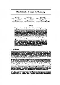
Figure 3.3: Comparison of size of k-best list for cube decoding with various feature sets.
substantially faster during decoding since these models do not search over trees, so we were able to use a larger range of k values for non-syntactic models. Scores improve when we increase k up to 10, but not much beyond. We observe that there is more benefit by adding feature sets than by increasing the value of k, as there is still a substantial gap (2.5 BLEU) between using phrase features with k = 20 and using all features with k = 5. This experiment is a preliminary result; we plan many more experiments along these lines in the thesis to compare k values in both cube summing and cube decoding.
3.2
Proposed Work
Cube summing is appealing in that it builds upon existing dynamic programming algorithms to compute expectations for models with non-local features. However, these expectations are biased and the bias is not yet well-understood. However, since we have relaxed requirements about associativity and distributivity and permit aggregation and combination operators to operate on sets, several extensions to cube summing become possible. First, when computing approximate summations with non-local features, we may not always be interested in the best proofs for each item. Since the purpose of summing is often to calculate statistics under a model distribution, we may wish instead to sample from that distribution. We can replace the max-k function with a sample-k function that samples k proofs from the scored list in its argument, possibly using the scores or possibly uniformly at random. These possibilities are ways to mitigate the bias in the expectations that are computed using cube summing. An alternative way to obtain unbiased estimators of expectations, or at least to better understand the bias that appears in practice, is to use Monte Carlo sampling methods for approximate inference. There are several classes of Monte Carlo inference algorithms. Markov chain Monte Carlo (MCMC) algorithms are used frequently in NLP for Bayesian inference, but are not wellsuited for handling non-local features, as described above. We instead turn to a class of Monte Carlo algorithms based on importance sampling. Before presenting our algorithm in §3.2.1, we will describe in more detail the class of models we are interested in. Many recent performance gains have resulted from working directly with efficient data structures representing the pruned search space of translation models. The search space for phrasebased models can be represented as a lattice and the space for systems that produce a parsed sentence can be represented as a hypergraph (Macherey et al., 2008; Tromble et al., 2008; Huang, 2008a; Kumar et al., 2009). A translation corresponds to a directed (hyper)path from a single start node to any of a number of final nodes in these representations. Feature locality is intuitive in these models; local features are restricted to individual edges, while non-local features can look at the entire path. To augment machine translation models with non-local features, we need an
3.2. PROPOSED WORK
21
approximate inference algorithm that supports computing expectations of non-local features in lattices and hypergraphs. Loopy belief propagation and MCMC algorithms are unnatural for this purpose, due to the many hard constraints imposed by the model. For example, for relatively sparse lattices, it may be very difficult to define Gibbs sampling moves to convert one path to another without requiring many other changes to reach a legal path (Chiang et al., 2010).
3.2.1
Importance Sampling
Importance sampling is a technique for estimating expectations with respect to a distribution that is difficult to sample from directly. Another distribution is used to draw samples, the samples are weighted using the original distribution of interest, and the expectations are estimated as weighted averages of the samples. Importance sampling is often used for directed graphical models, in which all potentials are locally normalized, while our primary interest is in feature-rich undirected models that are only normalized globally. We can still make use of importance sampling in this latter case, though with slightly worse theoretical guarantees. We begin with lattices for simplicity, but the technique also applies for inference in hypergraphs with non-local features that consider entire hyperpaths.6 Formally, a phrase lattice is a tuple hG, v0 , Vf , φi, in which G = (V, E) is a directed graph with vertex set V and edge multiset E,7 v0 ∈ V is the single initial vertex, Vf ⊆ V is the set of final vertexes, and φ : E → R≥0 is a nonnegative potential function assigning scores to edges. The traditional definition of a phrase lattice uses this definition of φ, but when using non-local features, we will redefine it as φ : P(E) → R≥0 , where P(E) is the power set of E excluding ∅. Each edge e ∈ E contains a phrase in the target language. A path from v0 to a vertex v ∈ Vf corresponds to a translation. We will use y to denote a path through the lattice; let y be a vector of indices in E of the sequence of edges crossed in the path. That is, eyi ∈ E is the ith edge crossed in the path y. We consider models of the form p(y) =
|y| 1 Y φ(ey1 , ..., eyi ) Z
(3.12)
i=1
where Z=
|y| XY
φ(ey1 , ..., eyi )
(3.13)
y∈H i=1
and where H is the set of all valid paths in G. Any feature can be included in this model, since the final term in the product, φ(ey1 , ..., ey|y| ), is a function of all edges in the path. We include the product with terms for each edge so as to capture the intuition that features “fire” as early as possible as the path is built up from start to finish; e.g., a feature that considers the first three edges will fire immediately upon seeing the third edge and so will be contained within the potential φ(ey1 , ey2 , ey3 ). Importance sampling is a procedure for estimating expectations of a function f (y) with respect to the distribution p(y) using samples, when p(y) is difficult to sample from directly. If we could sample from p(y), we could simply generate n samples {y (i) }ni=1 and estimate the expectation as 6 An importance sampling algorithm for linear-chain conditional random fields with non-local features is a special case of the algorithm we present for phrase lattices. 7 Multiple edges can exist with the same source and target vertexes but different target phrases and scores, so we use a multiset for E; this means that we will address edges by indices in E instead of the more common definition of edges as ordered pairs of vertexes.
22
CHAPTER 3. INFERENCE
follows:
n
1X f (y (i) ). n
Ep(y) [f (y)] ≈
(3.14)
i=1
If p(y) uses only local features, then we can sample from it by running the forward-backward algorithm once and then drawing as many samples as we wish (Goodman, 1998). However, p(y) is difficult to sample from directly when we use non-local features. Therefore, we will use importance sampling and sample from an alternative distribution and then weight the samples based on p(y). There are two settings of interest, one in which we can at least compute p(y), and the other in which we can only compute p(y) up to a multiplicative constant. When using globally-normalized models like the ones we consider here, we find ourselves in the latter setting.8 Nonetheless, we will describe both settings since the second builds upon the first. Importance Sampling When p(y) is Computable Importance sampling requires another distribution q(y) whose support is a superset of the support of p(y) and from which we can easily draw samples. We draw n samples y (1) , y (2) , ..., y (n) from q(y), which we will call the proposal distribution, then weight them according to the importance weight p(y) q(y) . Computinghthe expectation i of a function f (y) using the weighted samples is equivalent to estimating Eq(y) p(y) f (y) from q(y) unweighted samples and we therefore have an unbiased estimate: � X � X p(y) p(y) f (y) = q(y)f (y) = Eq(y) p(y)f (y) = Ep(y) [f (y)]. (3.15) q(y) q(y) y y For q(y), one simple option is to use a “locally-normalized” version of p(y). That is, define q(y) ,
|y| Y
φ(ey1 , ey2 , ..., eyi−1 , eyi ) j∈after (ey ) φ(ey1 , ey2 , ..., eyi−1 , ej )
P i=1
(3.16)
i−1
where after (e) returns the set of edges that can immediately follow e on a path. Sampling from q(y) can be performed by starting at v0 and sampling edges until reaching a final state; each edge is sampled from a multinomial distribution obtained through local normalization over all possible outgoing edges ej in the potential φ(ey1 , ey2 , ..., eyi−1 , ej ). Once a sample y has been obtained, some simple algebraic manipulation provides its weight: |y| p(y) 1 Y = wq (y) = q(y) Z
X
φ(ey1 , ey2 , ..., eyi−1 , ej ).
(3.17)
i=1 j∈after (eyi−1 )
Using these weights, we can estimate the expectation of f as follows: n
Ep(y) [f (y)] ≈
1X wq (y (i) )f (y (i) ). n
(3.18)
i=1
We see in Eq. 3.17 that the weight contains each of the normalization factors (for all i) in the denominator of Eq. 3.16. Since we already have to compute these terms to sample from q, we can use them immediately to compute the sample weights. Furthermore, the form of Eqs. 3.16 and 3.17 is amenable to a sequential implementation, in which we alternate between sampling an edge and weighting the resulting sample. This sequential nature allows resampling of samples to be easily incorporated, turning the algorithm into sequential importance sampling with resampling (SISR), also commonly known as particle filtering.9 8
The former setting could be useful for models in which Z is 1. We note that resampling is not as straightforward in the case of lattices as it is with sequence models and we leave the exploration of resampling strategies for the thesis. 9
3.2. PROPOSED WORK
23
Importance Sampling Without Computing p(y) Unfortunately, the weighting strategy in Eq. 3.17 is impractical for our model, because computing wq (y) requires being able to compute the partition function Z, which is intractable when using non-local features. So, we turn to another version of importance sampling for the case in which we can compute p(y) up to a multiplicative constant. That is, we can compute r(y), where r(y) Z = p(y) and wish again to compute expectations with respect to p(y). We sample from q(y) as before, but now weight by r(y)/q(y). Since Q|y| r(y) = i=1 φ(ey1 , ..., eyi ), the resulting weight will be: |y|
r(y) Y wr (y) = = q(y)
X
φ(ey1 , ey2 , ..., eyi−1 , ej ).
(3.19)
i=1 j∈after (eyi−1 )
The weights differ from those in Eq. 3.17 only by the absence of the term Z1 . This makes the implementation feasible, but comes with a price: the estimates are no longer unbiased when using a finite number of samples. To see this, consider the following: � X � X r(y) r(y) f (y) = q(y)f (y) = p(y)Zf (y) = ZEp(y) [f (y)]. (3.20) Eq(y) q(y) q(y) y y We do not have Z, but we can estimate it using the importance weights: � � X X r(y) r(y) Z= r(y) = q(y) = Eq(y) = Eq(y) [wr (y)] . q(y) q(y) y y Therefore, we can estimate the expectation of f as follows: Pn wr (y (i) )f (y (i) ) Pn . Ep(y) [f (y)] ≈ i=1 (i) i=1 wr (y )
(3.21)
For finite n, the estimates are biased, but as the number of samples goes to infinity, the bias disappears, decreasing as n1 (Koller and Friedman, 2009). Koller and Friedman also note that, while the estimater is biased, it often has smaller variance in practice than the unbiased estimator given above in Section 3.2.1; this reduction in variance often exceeds the bias of this method, making the biased sampler sometimes preferred over the unbiased sampler in practice. Finally, we note that alternative choices exist for q(y). One possibility is to use a stripped-down version of p(y) with only local features, which we will denote q` (y): |y| 1 Y q` (y) = φ(eyi ) Z`
(3.22)
i=1
where Z` =
|y| XY
φ(eyi )
(3.23)
y∈H i=1
and where H again is the set of all valid paths in G. The new weight wr` takes on the following form: |y| Y φ(ey1 , ..., eyi ) r(y) wr` (y) = = Z` . (3.24) q` (y) φ(eyi ) i=1
That is, we sample paths using the model with only local features, then weight each sample by the product of potentials for its non-local features. We also weight by Z` , which can be computed
24
CHAPTER 3. INFERENCE
efficiently by running the forward-backward algorithm on the lattice. The advantage of this approach is that we can use existing dynamic programming algorithms to help us sample from the model with only local features. As a starting point, we plan to compare these importance sampling algorithms for a simple model with features that are only “slightly” non-local, such as a phrase lattice with non-local features that consider two or three consecutive edges at a time. Since it is feasible (if expensive) to do exact inference with these non-local features for a small number of examples, we can measure the bias and variance of each algorithm’s estimates to perform a fair comparison. We also plan to include cube summing and mean-field variational inference (Wainwright and Jordan, 2008) in our comparison. In addition to looking at the accuracy of the expectation estimates, we will see which method gives the best results when those estimates are used for discriminative learning. We plan to use the results of these experiments to inform how we choose approximate inference methods for computing expectations of non-local features for phrase lattices and for our quasi-synchronous MT system from §2.
Chapter 4
Learning In this chapter, we propose two objective functions for training linear models for structured prediction. The first objective, which we call softmax-margin, is an extension of the standard conditional likelihood criterion for log-linear models that allows a task-specific cost function to be incorporated. It is a generalization of similar approaches used by Sha and Saul (2006) and Povey et al. (2008) for training speech recognition models. The second objective—which we call the Jensen risk bound—is a bound on risk via Jensen’s inequality that is easier to implement and more efficient to optimize than risk directly. We first discuss common training methods for linear models, focusing on methods used in MT (§4.1). We then describe softmax-margin (§4.2) and the Jensen risk bound (§4.3). We propose applying them to machine translation, both for phrase-based MT as well as our quasi-synchronous MT system from §2. We also propose using richer cost functions and training the relative weights for the different cost function components (§4.5).
4.1
Training Methods for Structured Linear Models
Let X denote a structured input space and, for a particular x ∈ X , let Y(x) denote a structured output space for x. The size of Y(x) is exponential in the size of x, which differentiates structured prediction from multiclass classification. For tree-to-string translation, for example, x might be a sentence with its parse and Y(x) the set of all translations. Where Y = ∪x∈X Y(x), we seek to learn a function h : X → Y that, given an x ∈ X , outputs a legal y ∈ Y(x). We use a linear model for h. That is, given a vector f (x, y) of feature functions on x and y and a parameter vector θ containing one component for each feature, the prediction yˆ for a new x is given by yˆ = argmax θ > f (x, y)
(4.1)
y∈Y(x)
By exponentiating and normalizing the score θ > f (x, y), we obtain a conditional log-linear model: exp{θ > f (x, y)} > 0 y 0 ∈Y(x) exp{θ f (x, y )}
pθ (y|x) = P
(4.2)
Many criteria exist for training the weights θ, which we will briefly review now. We assume a training set consisting of n input-output pairs {hx(i) , y (i) i}ni=1 . Some criteria will make use of a task-specific cost function that measures the extent to which a structure y differs from the true structure y (i) , denoted by cost(y (i) , y). Some criteria can use cost functions that consider a set of pairs and do not easily factor across training examples; we will overload cost to handle this situation, which should be clear from context. For machine translation, the cost function will 25
26
CHAPTER 4. LEARNING )n !
( MERT: min cost θ
Max-Margin: min θ
CL: min θ
Risk: min θ
Softmax-Margin: min θ
{y (i) }ni=1 ,
>
(i)
n X
� θ > f (x(i) , y) + cost(y (i) , y)
X
−θ > f (x(i) , y (i) ) + log
(4.4)
exp{θ > f (x(i) , y)}
(4.5)
y∈Y(x(i) )
X
exp{θ > f (x(i) , y)} (i) 0 > y 0 ∈Y(x(i) ) exp{θ f (x , y )}
cost(y (i) , y) P
i=1 y∈Y(x(i) ) n X > (i)
−θ f (x , y (i) ) + log
i=1
�
y∈Y(x(i) )
i=1 n X
i=1
−θ > f (x(i) , y (i) ) + max
i=1 n X
(4.3)
argmax θ f (x , y) y∈Y(x(i) )
X
(4.6)
exp{θ > f (x(i) , y) + cost(y (i) , y)}(4.7)
y∈Y(x(i) )
Figure 4.1: Objective functions for training linear models. Regularization terms (e.g., C are not shown here.
Pd
2 j=1 θj )
often be the negated BLEU score or an approximation thereof, but we plan to experiment with alternative cost functions as well. The most common approach to training translation models is minimum error rate training (MERT; Och, 2003). MERT refers to an algorithm for solving the optimization problem in Eq. 4.3. An advantage of MERT is that it can handle certain classes of document-level cost functions, including the negated BLEU score. However, MERT does not use regularization and has been observed to overfit, especially when using large numbers of features. In recent years, alternatives have been proposed for machine translation to attempt to address these deficiencies of MERT. One alternative is based on maximum-margin Markov networks (Taskar et al., 2003). The idea is to choose weights such that the linear score of each hx(i) , y (i) i is better than hx(i) , yi for all alternatives y ∈ Y(x(i) ) \ {y (i) }, with a larger margin for those y with higher cost. The “margin rescaling” form of this training criterion is shown in Eq. 4.4. A closely-related approach is the margin-infused relaxed algorithm (MIRA; Crammer et al., 2006), an online large-margin training algorithm that has recently shown success for training translation models (Watanabe et al., 2007; Arun and Koehn, 2007; Chiang et al., 2008, 2009). It can be shown that MIRA corresponds to a particular online learning algorithm for the structured max-margin objective of Eq. 4.4 (Martins et al., 2010). A related approach is the structured perceptron (Collins, 2002), which has also been used to train MT models (Liang et al., 2006; Tillmann and Zhang, 2006; Arun and Koehn, 2007). Another alternative is conditional likelihood (CL), commonly used when a probabilistic interpretation of the model is desired. The learning problem for maximizing conditional likelihood is shown in Eq. 4.5 (we transform it into a minimization problem for easier comparison). However, conditional likelihood cannot incorporate a cost function and has shown mixed results for training MT models (Smith and Eisner, 2006a; Zens et al., 2007; Blunsom et al., 2008; Blunsom and Osborne, 2008). An objective with a probabilistic interpretation that can make use of a cost function is risk. Risk is defined as the expected value of the cost with respect to the conditional distribution pθ (y|x). With a log-linear model, learning then requires solving the problem shown in Eq. 4.6. Unlike the
4.2. SOFTMAX-MARGIN
27
previous two criteria, risk is typically non-convex. As a result, the parameters reached by standard optimization procedures will depend on the initial values. This is also an issue with MERT, and it has been frequently noted in the community that MERT can achieve markedly different results when using different initial values. For MT, Smith and Eisner (2006a) minimized risk using k-best lists to define the distribution over output structures, and Li and Eisner (2009) introduced a novel semiring for minimizing risk using dynamic programming.
4.2
Softmax-Margin
The softmax-margin objective is shown as Eq. 4.7 and is a generalization of that used by Povey et al. (2008) and similar to that used by Sha and Saul (2006). The simple intuition is the same as the intuition in max-margin learning: high-cost outputs for x(i) should be penalized more heavily. Another view says that we replace the probabilistic score inside the exp function of CL with the “cost-augmented” score from max-margin. APthird view says that we replace the “hard” maximum of max-margin with the “softmax” (log exp) from CL; hence we use the name “softmaxmargin.” Like CL and max-margin, the objective is convex; a proof is provided in Gimpel and Smith (2010b). Softmax-margin training has a probabilistic interpretation, seen by situating it within the minimum divergence framework, which is a generalization of the well-known maximum entropy framework for learning (Jelinek, 1997). This connection is established in Gimpel and Smith (2010b).
4.2.1
Relation to Other Objectives
We next consider how softmax-margin upper bounds max-margin, CL, and risk. First, since the softmax function is a differentiable, convex upper bound on the max function, softmax-margin is a differentiable, convex upper bound on the max-margin objective. to CL and risk, we first define the following notation: let Zi = P To relate softmax-margin > (i) (i) y∈Y(x(i) ) exp{θ f (x , y)} and pi (·) = pθ (· | x ). We ignore the L2 penalty term below for clarity. We have: n X X −θ > f (x(i) , y (i) ) + log Softmax-Margin = exp{θ > f (x(i) , y) + cost(y (i) , y)} i=1
y∈Y(x(i) )
n X > (i) (i) = −θ f (x , y ) + log Zi
i=1
=
n � X
X
exp{θ > f (x(i) , y)} exp{cost(y (i) , y)}
y∈Y(x(i) )
Zi
n o� −θ > f (x(i) , y (i) ) + log Zi Epi [exp{cost(y (i) , ·)}]
i=1
=
n � X
>
(i)
(i)
�
−θ f (x , y ) + log Zi +
i=1
= CL +
n X
log Epi [exp{cost(y (i) , ·)}]
i=1 n X
log Epi [exp{cost(y (i) , ·)}]
(4.8)
i=1
We now focus on the last term. Since log is concave, we can use Jensen’s inequality to obtain, for all i: log Epi [exp{cost(y (i) , ·)}] ≥ Epi [log exp{cost(y (i) , ·)}] = Epi [cost(y (i) , ·)]
28
CHAPTER 4. LEARNING
Therefore,
n X
log Epi [exp{cost(y (i) , ·)}] ≥
i=1
Epi [cost(y (i) , ·)] = Risk
i=1
[exp{cost(y (i) , ·)}]
Since CL ≥ 0 and log Epi a convex bound on both risk and CL.
4.2.2
n X
≥ 0 (assuming cost is non-negative), softmax-margin is
Hidden Variables
We note that our feature-rich translation model from §2 treated word alignments as hidden variables and marginalized them out during conditional likelihood training. We now show how softmax-margin supports training with hidden variables. Ways of combining hidden variables with large-margin training have attracted interest in the machine learning community for several years, but only recently have principled approaches been presented (Zhu et al., 2008; Yu and Joachims, 2009). Unlike the latent-variable structured SVM of Yu and Joachims (2009) that finds the highest-scoring value for the latent variables, the softmax-margin approach marginalizes over all values. Where the hidden variable ranges over values h ∈ H(x) for an input x, softmax-margin with hidden variables is n X X X X − log min exp{θ > f (x(i) , y, h) + cost(y (i) , y)} exp{θ > f (x(i) , y (i) , h)} + log θ
i=1
y∈Yi h∈Hi
h∈Hi
where we have used Hi for H(x(i) ) and Yi for Y(x(i) ). We have assumed that cost does not depend on the hidden variable, as is commonly the case in NLP. If this is not the case, cost should be included in the numerator term and extended to take h as an additional argument. Like CL, extending softmax-margin with hidden variables causes it to be non-convex.
4.3
Jensen Risk Bound
We also be interesting to consider minimizing the function Pn note that it may (i) , ·)}] from Eq. 4.8, since it is an upper bound on risk but requires log E [exp{cost(y pi i=1 less computation to compute the gradient. We call this objective the Jensen risk bound (JRB). For a log-linear model, it takes the following form: n X X X log min exp{θ > f (x(i) , y) + cost(y (i) , y)} − log exp{θ > f (x(i) , y)} (4.9) θ
i=1
y∈Y(x(i) )
y∈Y(x(i) )
Like risk, this objective is not convex (being the difference of two convex functions), but its partial derivative with respect to a parameter θj for a single training pair hx(i) , y (i) i has an intuitive form: ∂ log Epi [exp{cost(y (i) , ·)}] = Epcost (·|x(i) ) [fj (x(i) , ·)] − Epθ (·|x(i) ) [fj (x(i) , ·)] θ ∂θj (i) where pcost θ (·|x ) is
(4.10)
exp{θ > f (x(i) , ·) + cost(y (i) , ·)} (i) 0 (i) 0 > y 0 ∈Y(x) exp{θ f (x , y ) + cost(y , y )}
P
When using this formula within gradient descent, we seek to decrease the weights of features that have larger expected values under the “cost-augmented” distribution over y than under the
4.4. EXPERIMENTS AND DISCUSSION
29 Cost
Method
Requirements
MERT Perceptron MIRA Max-Margin CL Risk Jensen Risk Bound Softmax-Margin
decoding decoding cost-augmented decoding cost-augmented decoding summing expectations of products cost-augmented summing cost-augmented summing
Function
Prob. Convex
Interp.
Permits Unreachable References X
X X X X
X X
X X X X X X
N/A X X X
X
Table 4.1: Comparison of training methods for linear models.
ordinary distribution without the cost function. The effect is that features that appear frequently in high-cost structures are penalized more heavily than features that mostly appear in low-cost structures. We note that, as with risk, the correct output structure y (i) is only accessed through the cost function; the feature vector for y (i) is not computed. This can be advantageous for situations in which the model may not be able to produce the actual y (i) , as is often the case in MT. In the experiments described in §2, we discarded a percentage of the training data that the model could not reach. We can contrast Eq. 4.10 with the analogous formula for minimizing risk: ∂Epi [cost(y (i) , ·)] = Epθ (·|x(i) ) [fj (x(i) , ·)cost(y (i) , ·)] − Epθ (·|x(i) ) [fj (x(i) , ·)]Epθ (·|x(i) ) [cost(y (i) , ·)] ∂θj (4.11) The presence of expectations of products makes computing Eq. 4.11 difficult for structured models. In fact, Li and Eisner (2009) developed a novel semiring solely for the purpose of computing these expectations of products. While their approach is elegant, it is non-trivial to implement, and regardless of implementation difficulty, minimizing risk for structured models remains a computationally expensive endeavor. We offer the Jensen risk bound as an alternative to risk that is easier to implement, requires less computation, and performs comparably in experiments conducted thus far.
4.4
Experiments and Discussion
We compared these training methods on a named-entity recognition task using the English data from the CoNLL 2003 shared task (Tjong Kim Sang and De Meulder, 2003). On test data, softmaxmargin is statistically indistinguishable from MIRA, risk, and JRB, but performs significantly better than CL, max-margin, and the perceptron. The Jensen risk bound performs comparably to risk, and takes roughly half as long to train. Additional experimental details for these results are provided in Gimpel and Smith (2010a). Table 4.1 shows a comparison of training methods in terms of their properties and requirements. The final two rows—the Jensen risk bound and softmax-margin—are contributions of this thesis. MERT, the perceptron, and max-margin learning only require decoding, making them attractive in terms of both implementation difficulty and computational requirements. However, they do not offer a probabilistic interpretation, which can be useful for computing posteriors and
30
CHAPTER 4. LEARNING
learning in the presence of hidden variables. One property that is particularly important for machine translation is whether the training method requires the gold standard translations to lie within the support of the model. MERT, risk, and the Jensen risk bound do not make this requirement, while the other methods do. Consequently, since the gold standard translations are often not reachable by the model, a surrogate oracle translation must be proposed in place of the gold standard for these other methods. For methods that require a gold standard, a fair amount of work has addressed the question of which oracle to choose, with several results suggesting that the oracle be a translation that scores highly under the automatic evaluation metric of interest and the current model parameters (Liang et al., 2006; Arun and Koehn, 2007; Chiang et al., 2008). This is typically captured either by choosing the oracle translation (under a particular metric) on an n-best list or a compact representation of the pruned search space such as a phrase lattice or hypergraph. We plan to experiment with various ways of choosing this oracle for methods which require it.
4.5
Proposed Work
We can use softmax-margin and the Jensen risk bound as drop-in replacements for conditional likelihood training of our quasi-synchronous translation model from §2. Hoping to make our contributions as generally applicable to MT as possible, we plan to first apply these training methods to learning the weights of the Moses phrase-based MT system (Koehn et al., 2007) by using phrase lattices to represent the space of possible translations. We plan to compare softmax-margin and the Jensen risk bound with the other training methods described above for these two training scenarios. We also plan to develop the notion of training with feature-rich cost functions as orthogonal to feature-rich modeling as is usually employed. While these cost features are not part of the model that gets used for prediction, they can bias the learning procedure to respect certain phenomena during training since they can look at the entire reference translation, something ordinary model features cannot do. We plan to experiment with cost features that model the standard BLEU metric (Papineni et al., 2001) as well as features that address synonymy, stemming, and paraphrase, which are components of the METEOR (Banerjee and Lavie, 2005) and TER-Plus (Snover et al., 2009) metrics, both of which have been shown to correlate better with human judgments than BLEU (Callison-Burch et al., 2009). It is an open question how to train the weights of the cost features; in our experiments thus far, we fixed their weights and experimented with several values. This has worked well for the simple cost functions we have used thus far, but we expect this to become prohibitively expensive for richer cost functions. In the thesis, we plan to address this question of how to train weights for cost features in a way that will be effective for translation and be applicable for other structured prediction models as well. Where T is the training data and D is the development data, one general formulation might be � � ˆ = argmax f2 D, argmin f1 (T, θ, λ) λ (4.12) λ
θ
where f1 is one of the cost-infused training objectives described above and f2 returns an evaluation metric score after decoding D using parameters given by its second argument. The traditional way to solve this problem is to treat λ as an additional set of hyperparameters of the experiment and use a grid search for optimal values. We will pursue alternative ways to optimize Eq. 4.12 to see whether a more efficient strategy can emerge.
Chapter 5
Summary of Proposed Work Component Features
Current Phrase, Target Syntax, Tree-to-Tree
Inference: Decoding
Cube decoding
Inference: Summing
Cube summing
Training
Conditional likelihood
Proposed See Table 2.4 Cube pruning and coarse-to-fine decoding Comparison of cube summing, importance sampling, and variational inference Comparison of several, including MERT, MIRA, softmax-margin, and Jensen risk bound
Table 5.1: Summary of proposed modifications to our quasi-synchronous machine translation system of §2. The primary focus of this thesis is to conduct experiments with our feature-rich quasisynchronous machine translation system from §2. Table 5.1 shows how our QG system currently looks and what we propose for the thesis, and Table 5.2 shows an estimated schedule for the proposed work. Preliminary results have been obtained using this framework, but a substantial amount of engineering will be required to improve performance to a position where these experiments can be meaningful for the community; we have allocated time for this engineering in the schedule. We expect the development of our inference and learning methods to have immediate application to our QG system as well as to benefit other approaches to translation. Therefore, we plan to initially demonstrate their effectiveness by applying them to phrase-based MT using the phrase lattice representation of the pruned search space describe in §3.2. This will also help us achieve our secondary goal of describing these methods generally enough that we can contribute to other structured problems in natural language processing and machine learning. We will use the results of these experiments to inform how to integrate the algorithms into our QG system. Once we have inference and learning methods integrated and have determined which methods work best with initial experiments, we plan to add features and conduct experiments for three language pairs. We propose to do German-to-English translation using data sets from the WMT shared tasks (Callison-Burch et al., 2009), Chinese-to-English translation using standard NIST data sets, and Urdu-to-English translation using NIST data as a contrastive small-data scenario. We plan to evaluate using not only the standard BLEU metric (Papineni et al., 2001), but also other metrics that have been shown to correlate better with human judgments, such as METEOR (Baner31
32
CHAPTER 5. SUMMARY OF PROPOSED WORK Semester
Summer 2010
Fall 2010
Spring 2011
Summer 2011
Fall 2011
Task §4.5
Description of Task
Writing §2.6
Write paper for EMNLP 2010 on phrase-based training
§3.2
Experiment with importance sampling for lattices for training phrasebased MT models with non-local features
Writing §2.6 §3.2, §4.5
Write paper for ACL 2011 on importance sampling
Writing
Write journal article on approximate inference methods for models with non-local features
§2.6
Add features to QG system from Table 2.4 and perform experiments with three language pairs
Writing
Write paper for EMNLP 2011 on feature-rich experiments with QG system
§4.5
Define and experiment with ways of training weights for cost features for training with feature-rich cost functions
Writing Other Defense
Write dissertation
Train phrase-based models with softmax-margin and Jensen risk bound within lattice training framework Improve efficiency of QG decoder with cube pruning and coarse-to-fine decoding
Experiment with QG system and engineer to improve performance Incorporate most successful inference and learning techniques into QG system
Job search November 2011
Table 5.2: Timeline for proposed work.
jee and Lavie, 2005), TER (Snover et al., 2006), and TER-Plus (Snover et al., 2009).
Bibliography Alshawi, H., Bangalore, S., and Douglas, S. (2000). Learning dependency translation models as collections of finite-state head transducers. Computational Linguistics, 26(1):45–60. [6] Arun, A. and Koehn, P. (2007). Online learning methods for discriminative training of phrase based statistical machine translation. In Proc. of MT Summit XI. [26, 30] Banerjee, S. and Lavie, A. (2005). METEOR: An automatic metric for MT evaluation with improved correlation with human judgments. In Proc. of ACL Workshop on Intrinsic and Extrinsic Evaluation Measures for MT and/or Summarization. [3, 9, 30, 31] Besag, J. E. (1975). Statistical analysis of non-lattice data. The Statistician, 24:179–195. [8] Blunsom, P., Cohn, T., and Osborne, M. (2008). A discriminative latent variable model for statistical machine translation. In Proc. of ACL. [10, 26] Blunsom, P. and Osborne, M. (2008). Probabilistic inference for machine translation. In Proc. of EMNLP. [18, 26] Callison-Burch, C., Koehn, P., Monz, C., and Schroeder, J. (2009). Findings of the 2009 Workshop on Statistical Machine Translation. In Proc. of the Fourth Workshop on Statistical Machine Translation. [30, 31] Carreras, X., Collins, M., and Koo, T. (2008). TAG, dynamic programming, and the perceptron for efficient, feature-rich parsing. In Proc. of CoNLL. [1] Charniak, E. and Johnson, M. (2005). Coarse-to-fine n-best parsing and maxent discriminative reranking. In Proc. of ACL. [11] Chen, S. and Goodman, J. (1998). An empirical study of smoothing techniques for language modeling. Technical report 10-98, Harvard University. [9] Chiang, D. (2005). A hierarchical phrase-based model for statistical machine translation. In Proc. of ACL. [i, 1, 2, 12] Chiang, D. (2007). Hierarchical phrase-based translation. Computational Linguistics, 33(2):201–228. [2, 4, 8, 9, 13, 14, 16, 17] Chiang, D. (2010). Learning to translate with source and target syntax. In Proc. of ACL. [4] Chiang, D., Graehl, J., Knight, K., Pauls, A., and Ravi, S. (2010). Bayesian inference for finite-state transducers. In Proc. of NAACL. [21] Chiang, D., Marton, Y., and Resnik, P. (2008). Online large-margin training of syntactic and structural translation features. In Proc. of EMNLP. [26, 30] Chiang, D., Wang, W., and Knight, K. (2009). 11,001 new features for statistical machine translation. In Proc. of NAACL-HLT. [3, 26] Collins, M. (1999). Head-Driven Statistical Models for Natural Language Parsing. PhD thesis, U. Penn. [9] Collins, M. (2002). Discriminative training methods for hidden Markov models: Theory and experiments with perceptron algorithms. In Proc. of EMNLP. [26] 33
34
BIBLIOGRAPHY
Crammer, K., Dekel, O., Keshet, J., Shalev-Shwartz, S., and Singer, Y. (2006). Online passiveaggressive algorithms. Journal of Machine Learning Research, 7:551–585. [-] Darwiche, A. (2003). A differential approach to inference in Bayesian networks. Journal of the ACM, 50(3). [19] DeNeefe, S. and Knight, K. (2009). Synchronous tree adjoining machine translation. In Proc. of EMNLP. [i, 1] Ding, Y. and Palmer, M. (2005). Machine translation using probabilistic synchronous dependency insertion grammar. In Proc. of ACL. [6] Eisner, J. (1997). Bilexical grammars and a cubic-time probabilistic parser. In Proc. of IWPT. [7] Finkel, J. R., Grenager, T., and Manning, C. D. (2005). Incorporating non-local information into information extraction systems by gibbs sampling. In Proc. of ACL. [13] Galley, M., Graehl, J., Knight, K., Marcu, D., DeNeefe, S., Wang, W., and Thayer, I. (2006). Scalable inference and training of context-rich syntactic translation models. In Proc. of COLING-ACL. [i, 1, 4, 5] Gimpel, K. and Smith, N. A. (2009a). Cube summing, approximate inference with non-local features, and dynamic programming without semirings. In Proc. of EACL. [i, 2, 4, 9, 14, 17, 19] Gimpel, K. and Smith, N. A. (2009b). Feature-rich translation by quasi-synchronous lattice parsing. In Proc. of EMNLP. [i, 2, 8, 9] Gimpel, K. and Smith, N. A. (2010a). Softmax-margin CRFs: Training log-linear models with cost functions. In Proc. of NAACL. [i, 2, 29] Gimpel, K. and Smith, N. A. (2010b). Softmax-margin training for structured log-linear models. Technical report, Carnegie Mellon University. [27] Goodman, J. (1998). Parsing inside-out. PhD thesis, Harvard University. [19, 22] Goodman, J. (1999). Semiring parsing. Computational Linguistics, 25(4):573–605. [14] Huang, L. (2008a). Forest-based Algorithms in Natural Language Processing. PhD thesis, University of Pennsylvania. [20] Huang, L. (2008b). Forest reranking: Discriminative parsing with non-local features. In Proc. of ACL. [i, 1, 13] Huang, L. and Chiang, D. (2007). Forest rescoring: Faster decoding with integrated language models. In Proc. of ACL. [2, 13, 14, 16, 17] Huang, L., Knight, K., and Joshi, A. (2006). Statistical syntax-directed translation with extended domain of locality. In Proc. of AMTA. [i, 1, 4] Jelinek, F. (1997). Statistical methods for speech recognition. MIT Press. [27] Klein, D. and Manning, C. D. (2003). Fast exact inference with a factored model for natural language parsing. In Advances in NIPS 15. [9] Klein, D. and Manning, C. D. (2004). Corpus-based induction of syntactic structure: Models of dependency and constituency. In Proc. of ACL. [9, 12] Koehn, P., Hoang, H., Birch, A., Callison-Burch, C., Federico, M., Bertoldi, N., Cowan, B., Shen, W., Moran, C., Zens, R., Dyer, C., Bojar, O., Constantin, A., and Herbst, E. (2007). Moses: Open source toolkit for statistical machine translation. In Proc. of ACL (demo session). [2, 5, 7, 9, 30] Koehn, P., Och, F. J., and Marcu, D. (2003). Statistical phrase-based translation. In Proc. of HLTNAACL. [i, 4, 12] Koller, D. and Friedman, N. (2009). Probabilistic Graphical Models: Principles and Techniques. MIT Press. [13, 23]
BIBLIOGRAPHY
35
Kumar, S., Macherey, W., Dyer, C., and Och, F. (2009). Efficient minimum error rate training and minimum Bayes-risk decoding for translation hypergraphs and lattices. In Proc. of ACL-IJCNLP. [20] Li, Z. and Eisner, J. (2009). First- and second-order expectation semirings with applications to minimum-risk training on translation forests. In Proc. of EMNLP. [i, 2, 3, 27, 29] ˆ e, A., Klein, D., and Taskar, B. (2006). An end-to-end discriminative apLiang, P., Bouchard-Cot´ proach to machine translation. In Proc. of COLING-ACL. [26, 30] ¨ Y., and Liu, Q. (2009). Improving tree-to-tree translation with packed forests. In Proc. Liu, Y., Lu, of ACL-IJCNLP. [i, 1, 4] Macherey, W., Och, F., Thayer, I., and Uszkoreit, J. (2008). Lattice-based minimum error rate training for statistical machine translation. In EMNLP. [20] Marcu, D., Wang, W., Echihabi, A., and Knight, K. (2006). Statistical machine translation with syntactified target language phrases. In Proc. of EMNLP. [5] Martins, A. F. T., Gimpel, K., Smith, N. A., Xing, E. P., Aguiar, P. M. Q., and Figueiredo, M. A. T. (2010). Learning structured classifiers with dual coordinate descent. Technical report, Carnegie Mellon University. [26] Martins, A. F. T., Smith, N. A., and Xing, E. P. (2009). Concise integer linear programming formulations for dependency parsing. In Proc. of ACL. [i, 1, 13] Mi, H., Huang, L., and Liu, Q. (2008). Forest-based translation. In Proc. of ACL. [5] NIST (2009). NIST 2009 machine translation evaluation official results. [1] Och, F. J. (2003). Minimum error rate training for statistical machine translation. In Proc. of ACL. [-] Och, F. J. and Ney, H. (2003). A systematic comparison of various statistical alignment models. Computational Linguistics, 29(1). [9] Papineni, K., Roukos, S., Ward, T., and Zhu, W. (2001). BLEU: a method for automatic evaluation of machine translation. In Proc. of ACL. [3, 9, 30, 31] Petrov, S. (2009). Coarse-to-Fine Natural Language Processing. PhD thesis, University of California at Berkeley. [11, 13] Povey, D., Kanevsky, D., Kingsbury, B., Ramabhadran, B., Saon, G., and Visweswariah, K. (2008). Boosted MMI for model and feature space discriminative training. In Proc. of ICASSP. [25, 27] Quirk, C., Menezes, A., and Cherry, C. (2005). Dependency treelet translation: Syntactically informed phrasal SMT. In Proc. of ACL. [2, 5, 12] Roth, D. and Yih, W. (2004). A linear programming formulation for global inference in natural language tasks. In Proc. of CoNLL. [13] Sha, F. and Saul, L. K. (2006). Large margin hidden Markov models for automatic speech recognition. In Proc. of NIPS. [25, 27] Shen, L., Xu, J., and Weischedel, R. (2008). A new string-to-dependency machine translation algorithm with a target dependency language model. In Proc. of ACL. [i, 1, 2, 4, 5, 12] Shieber, S., Schabes, Y., and Pereira, F. (1995). Principles and implementation of deductive parsing. Journal of Logic Programming, 24(1-2):3–36. [14] Smith, D. A. and Eisner, J. (2006a). Minimum risk annealing for training log-linear models. In Proc. of COLING-ACL. [2, 3, 26, 27] Smith, D. A. and Eisner, J. (2006b). Quasi-synchronous grammars: Alignment by soft projection of syntactic dependencies. In Proc. of HLT-NAACL Workshop on Statistical Machine Translation. [6, 10, 11, 12]
36
BIBLIOGRAPHY
Smith, D. A. and Eisner, J. (2008). Dependency parsing by belief propagation. In Proc. of EMNLP. [13] Snover, M., Dorr, B., Schwartz, R., Micciulla, L., and Makhoul, J. (2006). A study of translation edit rate with targeted human annotation. In Proc. of AMTA. [3, 32] Snover, M., Madnani, N., Dorr, B., and Schwartz, R. (2009). Fluency, adequacy, or HTER? exploring different human judgments with a tunable MT metric. In Proc. of WMT. [3, 30, 32] Stolcke, A. (2002). SRILM—an extensible language modeling toolkit. In Proc. of ICSLP. [9] Sutton, C. and McCallum, A. (2004). Collective segmentation and labeling of distant entities in information extraction. In Proc. of ICML Workshop on Statistical Relational Learning and Its Connections to Other Fields. [13] Taskar, B., Guestrin, C., and Koller, D. (2003). Max-margin Markov networks. In Advances in NIPS 16. [26] Tillmann, C. and Zhang, T. (2006). A discriminative global training algorithm for statistical MT. In Proc. of COLING-ACL. [26] Tjong Kim Sang, E. F. and De Meulder, F. (2003). Introduction to the CoNLL-2003 shared task: Language-independent named entity recognition. In Proc. of CoNLL. [29] Tromble, R., Kumar, S., Och, F., and Macherey, W. (2008). Lattice Minimum Bayes-Risk decoding for statistical machine translation. In EMNLP. [20] Wainwright, M. J. and Jordan, M. I. (2008). Graphical models, exponential families, and variational inference. Foundations and Trends in Machine Learning. Now Publishers. [24] Watanabe, T., Suzuki, J., Tsukada, H., and Isozaki, H. (2007). Online large-margin training for statistical machine translation. In Proc. of EMNLP-CoNLL. [26] Yamada, K. and Knight, K. (2001). A syntax-based statistical translation model. In Proc. of ACL. [1] Yu, C. J. and Joachims, T. (2009). Learning structural SVMs with latent variables. In Proc. of ICML. [28] Zens, R., Hasan, S., and Ney, H. (2007). A systematic comparison of training criteria for statistical machine translation. In Proc. of EMNLP. [26] Zhu, J., Xing, E. P., , and Zhang, B. (2008). Partially observed maximum entropy discrimination markov networks. In Proc. of NIPS. [28] Zollmann, A. and Venugopal, A. (2006). Syntax augmented machine translation via chart parsing. In Proc. of NAACL 2006 Workshop on Statistical Machine Translation. [i, 1, 4, 5]