Discriminative Features for GMM and i-Vector based Speaker Diarization

Ph.D. Thesis

Discriminative Features for GMM and i-Vector based Speaker Diarization

Author: Abraham Woubie Zewoudie

Advisors: Prof. Francisco Javier Hernando Pericas Dr. Jordi Luque Serrano

TALP Research Center, Speech Processing Group Department of Signal Theory and Communications Universitat Politècnica de Catalunya, Barcelona, Spain

June, 2017

To my family and wife

iii

Abstract Speaker diarization has received several research attentions over the last decade. Among the different domains of speaker diarization, diarization in meeting domain is the most challenging one. It usually contains spontaneous speech and is, for example, susceptible to reverberation. The appropriate selection of speech features is one of the factors that affect the performance of speaker diarization systems. Mel Frequency Cepstral Coefficients (MFCC) are the most widely used short-term speech features in speaker diarization. Other factors that affect the performance of speaker diarization systems are the techniques employed to perform both speaker segmentation and speaker clustering. In this thesis, we have proposed the use of jitter and shimmer long-term voice-quality features both for GMM and i-vector based speaker diarization systems. The voicequality features are used together with the state-of-the-art short-term cepstral and longterm speech ones. The long-term features consists of prosody and Glottal-to-Noise excitation ratio (GNE) descriptors. Firstly, the voice-quality, prosodic and GNE features are stacked in the same feature vector. Then, they are fused with cepstral coefficients at the score likelihood level both for the proposed Gaussian Mixture Modeling (GMM) and i-vector based speaker diarization systems. For the proposed GMM based speaker diarization system, independent HMM models are estimated from each set of features. In speaker segmentation, the fusion of the short-term descriptors with the long-term ones is carried out by linearly weighting the log-likelihood scores of Viterbi decoding. In speaker clustering, the fusion of the shortterm cepstral features with the long-term ones is carried out by linearly fusing the BIC scores corresponding to these feature sets. For the proposed i-vector based speaker diarization system, the feature fusion is performed exactly the same as the one in the previously mentioned GMM based system. But, the speaker clustering technique is based on the recently introduced factor analysis paradigm. Two sets of i-vectors are extracted from the speaker segmentation hypothesis. v

vi Whilst the first i-vector is extracted from short-term spectral features, the second one is extracted from the stacked voice quality, prosodic and GNE descriptors. Then, the cosine-distance and Probabilistic Linear Discriminant Analysis (PLDA) scores among ivectors are linearly weighted to obtain a unique similarity score. Finally, the final fused score is used as speaker clustering distance. We have also proposed the use of delta dynamic features for speaker clustering. The motivation for using deltas in clustering is because they capture the transitional characteristics of the speech about speaker specific information. The proposed speaker diarization system uses both the static and delta dynamic features for speaker clustering. The speaker segmentation is based only on the static MFCC feature set. The experiments have been carried out on Augmented Multi-party Interaction (AMI) meeting corpus. The experimental results show that the use of voice-quality, prosodic, GNE and delta dynamic features improve the performance of both GMM and i-vector based speaker diarization systems.

Resumen La diarizaci´ on del altavoz ha recibido varias atenciones de investigación durante la u ´ltima década. Entre los diferentes dominios de la diarización del hablante, la diarización en el dominio del encuentro es la m´ as dif´ıcil. Normalmente contiene habla espontánea y, por ejemplo, es susceptible de reverberación. La selecci´ on apropiada de las caracter´ısticas del habla es uno de los factores que afectan el rendimiento de los sistemas de diarización de los altavoces. Los Coeficientes Cepstral de Frecuencia Mel (MFCC) son las caracter´ısticas de habla de corto plazo más utilizadas en la diarizaci´ on de los altavoces. Otros factores que afectan el rendimiento de los sistemas de diarizaci´ on del altavoz son las técnicas empleadas para realizar tanto la segmentaci´ on del altavoz como el agrupamiento de altavoces. En esta tesis, hemos propuesto el uso de jitter y shimmer caracter´ısticas de calidad de voz a largo plazo tanto para GMM y i-vector basada en sistemas de diarización de altavoces. Las caracter´ısticas de calidad de voz se utilizan junto con el estado de la técnica a corto plazo cepstral y de larga duración de habla. Las caracter´ısticas a largo plazo consisten en la prosodia y los descriptores de relación de excitación Glottal-a-Ruido (GNE). En primer lugar, las caracter´ısticas de calidad de voz, prosódica y GNE se apilan en el mismo vector de caracter´ısticas. A continuación, se fusionan con coeficientes cepstrales en el nivel de verosimilitud de puntajes tanto para los sistemas de diarización de altavoces basados en el modelo Gaussian Mixture Modeling (GMM) como en los sistemas basados en i. Para el sistema de diarizaci´ on de altavoces basado en GMM propuesto, se calculan modelos HMM independientes a partir de cada conjunto de caracter´ısticas. En la segmentaci´ on de los altavoces, la fusión de los descriptores a corto plazo con los de largo plazo se lleva a cabo mediante la ponderación lineal de las puntuaciones log-probabilidad de decodificaci´ on Viterbi. En la agrupación de altavoces, la fusión de las caracter´ısticas cepstrales a corto plazo con las de largo plazo se lleva a cabo mediante la fusión lineal de las puntuaciones BIC correspondientes a estos conjuntos de caracter´ısticas.

vii

viii Para el sistema de diarizaci´ on de altavoces basado en un vector i, la fusión de caracter´ısticas se realiza exactamente igual a la del sistema basado en GMM antes mencionado. Sin embargo, la técnica de agrupación de altavoces se basa en el paradigma de análisis de factores recientemente introducido. Dos conjuntos de i-vectores se extraen de la hip´ otesis de segmentaci´ on de altavoz. Mientras que el primer vector i se extrae de caracter´ısticas espectrales a corto plazo, el segundo se extrae de los descriptores de calidad de voz apilados, pros´ odicos y GNE. A continuación, las puntuaciones de coseno-distancia y Probabilistic Linear Discriminant Analysis (PLDA) entre i-vectores se ponderan linealmente para obtener una puntuación de similitud u ńica. Finalmente, la puntuación final fusionada se utiliza como distancia de agrupación de altavoces. También hemos propuesto el uso de caracter´ısticas dinámicas delta para el agrupamiento de altavoces. La motivaci´ on para usar deltas en la agrupación es porque capturan las caracter´ısticas de transici´ on del discurso sobre la información espec´ıfica del hablante. El sistema de diarizaci´ on de altavoces propuesto utiliza tanto las caracter´ısticas dinámicas estáticas como delta para la agrupaci´ on de altavoces. La segmentación del altavoz se basa u ńicamente en el conjunto de funciones MFCC estáticas. Los experimentos se han llevado a cabo en el corpus de reunión de interacción multipartito aumentada (AMI). Los resultados experimentales muestran que el uso de calidad vocal, prosódica, GNE y din´ amicas delta mejoran el rendimiento de los sistemas de diarización de altavoces basados en GMM e i-vector.

Acknowledgements First and above all, I praise the Almighty God for providing me this opportunity and capability to complete my PhD successfully. Then, I would like to thank my thesis advisors Javier Hernando and Jordi Luque for giving me the opportunity to do my Ph.D. at the Speech Processing Research Group of The Center for Language and Speech Technologies and Applications (TALP) research center in UPC BarcelonaTech. Working with them was a great experience, and I am grateful for their time, patience, dedication and passion until the completion of my PhD. Doing Ph.D. at UPC gave me a chance to meet wonderful people who have made this journey memorable. I would like to express my gratitude to Catalan Government and UPC for funding my Ph.D study. Many thanks also to Climent Nadeu, Antonio Bonafonte, Luis Torres, Miquel and Umair Khan for their friendship and camaraderie over the past four years. Last but not the least, I would like to thank my parents Woubie Zewoudie and Azeb Manaye for their unconditional love and care. I would not have made it this far without their support. Finally, I would like to thank my wife Etsub for standing beside me throughout my four years in UPC. She has been my inspiration and motivation. She is my rock, and I dedicate this PhD dissertation to her.

ix

Contents Abstract

v

Resumen

vii

Acknowledgements

ix

List of Figures

xiii

List of Tables

xv

1 Introduction 1.1 Motivation and Objectives . . . . . . . . . . . . . . . . . . . . . . . . . . . 1.2 Publications from the thesis . . . . . . . . . . . . . . . . . . . . . . . . . . 1.3 Organization of the thesis . . . . . . . . . . . . . . . . . . . . . . . . . . . 2 State-of-the-art in Speaker Diarization 2.1 Speaker Diarization . . . . . . . . . . . . . . 2.2 Speech Features . . . . . . . . . . . . . . . . 2.2.1 Short-term Speech Features . . . . . 2.2.2 Long-term Speech Features . . . . . 2.3 Speech/Non-speech detection . . . . . . . . 2.4 Speaker Modeling Techniques . . . . . . . . 2.4.1 Gaussian Mixture Modeling . . . . . 2.4.2 i-Vector . . . . . . . . . . . . . . . . 2.4.3 Speaker Factors . . . . . . . . . . . . 2.4.4 Artificial Neural Networks . . . . . . 2.4.5 Deep Neural Networks . . . . . . . . 2.5 Speaker Segmentation . . . . . . . . . . . . 2.6 Speaker Clustering . . . . . . . . . . . . . . 2.7 Approaches to Speaker Diarization System . 2.8 Evaluation Metrics . . . . . . . . . . . . . . 3 The 3.1 3.2 3.3 3.4 3.5

. . . . . . . . . . . . . . .

. . . . . . . . . . . . . . .

. . . . . . . . . . . . . . .

UPC Baseline Speaker Diarization System Front-end Processing . . . . . . . . . . . . . . . . Cluster Initialization . . . . . . . . . . . . . . . . Iterative Viterbi-Segmentation . . . . . . . . . . Speaker Clustering . . . . . . . . . . . . . . . . . Merging and Stopping Criterion . . . . . . . . . . xi

. . . . . . . . . . . . . . .

. . . . .

. . . . . . . . . . . . . . .

. . . . .

. . . . . . . . . . . . . . .

. . . . .

. . . . . . . . . . . . . . .

. . . . .

. . . . . . . . . . . . . . .

. . . . .

. . . . . . . . . . . . . . .

. . . . .

. . . . . . . . . . . . . . .

. . . . .

. . . . . . . . . . . . . . .

. . . . .

. . . . . . . . . . . . . . .

. . . . .

. . . . . . . . . . . . . . .

. . . . .

. . . . . . . . . . . . . . .

. . . . .

. . . . . . . . . . . . . . .

. . . . .

. . . . . . . . . . . . . . .

. . . . .

1 2 5 8

. . . . . . . . . . . . . . .

11 11 12 12 13 16 17 18 20 26 27 28 29 33 35 37

. . . . .

41 42 43 45 46 48

xii

Contents

4 Long-term Speech Features for Speaker Diarization 4.1 Dynamic Features . . . . . . . . . . . . . . . . . . . . 4.2 Voice-quality . . . . . . . . . . . . . . . . . . . . . . . 4.2.1 Jitter . . . . . . . . . . . . . . . . . . . . . . . 4.2.2 Shimmer . . . . . . . . . . . . . . . . . . . . . 4.3 Prosody . . . . . . . . . . . . . . . . . . . . . . . . . . 4.3.1 Pitch . . . . . . . . . . . . . . . . . . . . . . . . 4.3.2 Acoustic intensity . . . . . . . . . . . . . . . . 4.3.3 Formant Frequencies . . . . . . . . . . . . . . . 4.4 Glottal-to-Noise Excitation Ratio . . . . . . . . . . . .

. . . . . . . . .

. . . . . . . . .

. . . . . . . . .

. . . . . . . . .

. . . . . . . . .

. . . . . . . . .

. . . . . . . . .

. . . . . . . . .

. . . . . . . . .

. . . . . . . . .

. . . . . . . . .

51 53 54 56 57 58 60 61 61 62

5 Proposed Speaker Diarization Systems 5.1 Fusion Techniques . . . . . . . . . . . . . . . . . . . 5.1.1 Feature Level Fusion . . . . . . . . . . . . . . 5.1.2 Score Level Fusion . . . . . . . . . . . . . . . 5.2 Proposed HMM/GMM Speaker Diarization System . 5.2.1 Feature Extraction . . . . . . . . . . . . . . . 5.2.2 Speaker Segmentation . . . . . . . . . . . . . 5.2.3 Speaker Clustering . . . . . . . . . . . . . . . 5.3 Proposed i-Vector based Speaker Diarization System 5.3.1 Speaker Clustering . . . . . . . . . . . . . . .

. . . . . . . . .

. . . . . . . . .

. . . . . . . . .

. . . . . . . . .

. . . . . . . . .

. . . . . . . . .

. . . . . . . . .

. . . . . . . . .

. . . . . . . . .

. . . . . . . . .

. . . . . . . . .

. . . . . . . . .

67 67 68 68 69 71 72 72 73 74

6 Experimental Setups and Results 6.1 Augmented Meeting Corpus (AMI) Corpus . . . 6.2 HMM/GMM based Speaker Diarization Systems 6.2.1 Experimental Setup . . . . . . . . . . . . 6.2.2 Delta Features Results . . . . . . . . . . . 6.2.3 Jitter and Shimmer Results . . . . . . . . 6.2.4 Prosody Results . . . . . . . . . . . . . . 6.2.5 Voice-quality and Prosody Results . . . . 6.3 i-Vector based Speaker Diarization Systems . . . 6.3.1 Experimental Setup . . . . . . . . . . . . 6.3.2 i-Vector based Cosine Distance Clustering 6.3.3 i-Vector based PLDA Clustering . . . . .

. . . . . . . . . . .

. . . . . . . . . . .

. . . . . . . . . . .

. . . . . . . . . . .

. . . . . . . . . . .

. . . . . . . . . . .

. . . . . . . . . . .

. . . . . . . . . . .

. . . . . . . . . . .

. . . . . . . . . . .

. . . . . . . . . . .

. . . . . . . . . . .

79 79 80 81 82 83 84 85 87 88 89 92

. . . . . . . . . . .

. . . . . . . . . . .

7 Conclusions and Future works 99 7.1 Conclusions . . . . . . . . . . . . . . . . . . . . . . . . . . . . . . . . . . . 99 7.2 Future Research Lines . . . . . . . . . . . . . . . . . . . . . . . . . . . . . 102

Appendices

105

A AMI Partitions Used

107

Bibliography

109

List of Figures 2.1 2.2 2.3 2.4 2.5 2.6 2.7 2.8 2.9

Speaker segmentation and clustering example. . . . Example of speaker model adaptation. . . . . . . . The i-vector extraction process. . . . . . . . . . . . Example of PLDA Model . . . . . . . . . . . . . . . Speaker factor extraction process. . . . . . . . . . . Example of Artificial Neural Network. . . . . . . . Example of audio signal with three speakers. . . . . Example of ∆ BIC Values. . . . . . . . . . . . . . . Bottom-Up and Top-down approaches to clustering

3.1 3.2 3.3 3.4

The UPC baseline speaker diarization system architecture. . . . . . . . . Ergodic HMM/GMM system with a minimum duration constraint. . . . Example of minimum duration constraint. . . . . . . . . . . . . . . . . . DER results on NIST Transcription 2006 and 2007 evaluation conference data using the minimum duration into account in the HMM decoding. .

. 42 . 45 . 46

4.1 4.2 4.3 4.4 4.5

The process of Delta feature extraction. . . Jitter measurements for 3 pitch periods . . Shimmer measurements for 3 pitch periods Example of prosodic features. . . . . . . . Process of GNE extraction. . . . . . . . .

. . . . .

5.1 5.2

Example of feature level fusion. . . . . . . . . . . . . . . . . . . . . . . . Proposed HMM/GMM based speaker diarization system using short- and long-term term speech features. . . . . . . . . . . . . . . . . . . . . . . . Proposed i-vector based speaker clustering architecture based on a weighted cosine-distance among i-vectors. . . . . . . . . . . . . . . . . . . . . . . . Proposed i-vector based speaker clustering architecture based on a weighted PLDA scores among i-vectors. . . . . . . . . . . . . . . . . . . . . . . . .

5.3 5.4

6.1 6.2 6.3 6.4

. . . . .

. . . . .

. . . . .

. . . . .

. . . . .

. . . . . . . . .

. . . . .

. . . . . . . . .

. . . . .

. . . . . . . . .

. . . . .

. . . . . . . . .

. . . . .

. . . . . . . . .

. . . . .

. . . . . . . . .

. . . . .

. . . . . . . . .

. . . . .

. . . . . . . . .

. . . . .

. . . . . . . . .

. . . . .

. . . . . . . . .

. . . . .

. . . . . . . . .

. . . . .

. . . . . . . . .

. . . . .

DER of the development and test sets for HMM/GMM speaker diarization system using MFCC, JS and prosodic feature sets. . . . . . . . . . . . . Box plot of the development and test sets for HMM/GMM speaker diarization system using MFCC, JS and prosodic feature sets. . . . . . . . DER and cosine-distance score per iteration for selected shows from the development set. . . . . . . . . . . . . . . . . . . . . . . . . . . . . . . . DER Comparison of GMM based BIC and i-vector based cosine distance (CD) clustering using MFCC, JS and prosodic feature sets. . . . . . . .

xiii

. . . . . . . . .

12 19 23 24 26 27 31 32 34

. 47 54 57 58 62 63

. 68 . 70 . 75 . 76

. 85 . 87 . 89 . 91

xiv

List of Figures 6.5 6.6 6.7

DER of the test set for GMM and i-vector based speaker clustering techniques using MFCC, JS, prosodic and GNE feature sets. . . . . . . . . . . 94 Box plot of the development and test using GMM and i-vector based clustering techniques using MFCC and Long-Term Speech Features (LT). . . . 95 Box Plot of the chunks test set for GMM based BIC and i-vector based PLDA clustering techniques using MFCC, JS, Prosodic and GNE features. 96

List of Tables 5.1

The proposed GMM and i-vector based speaker diariaztion systems and the score fusion techniques carried out in segmentation and clustering. . 69

6.1

DER of the test sets for HMM/GMM speaker diarization system using MFCC and MFCC + Delta (∆) feature set. . . . . . . . . . . . . . . . . . DER of the development and test sets for HMM/GMM speaker diarization system using MFCC, and Jitter and Shimmer (JS) feature sets. . . . . . . DER of the development and test sets for HMM/GMM speaker diarization system using MFCC and prosodic feature sets. . . . . . . . . . . . . . . . DER of the development and test sets for HMM/GMM speaker diarization system using MFCC, JS and prosodic feature sets. . . . . . . . . . . . . . DER of the development set for GMM based BIC and i-vector based cosine distance clustering techniques using MFCC, JS and prosodic feature sets. . DER of the test set for GMM based BIC and i-vector based cosine distance clustering techniques using MFCC, JS and prosodic feature sets. . . . . . DER of the chunk test set for GMM based BIC and i-vector based cosine distance clustering techniques using MFCC, JS and prosodic feature sets. . DER of the development set for GMM and i-vector based speaker clustering techniques using MFCC, JS, prosodic and GNE feature sets. . . . . . . DER of the chunk test set for GMM and i-vector based speaker clustering techniques using MFCC, JS, prosodic and GNE feature sets. . . . . . . . .

6.2 6.3 6.4 6.5 6.6 6.7 6.8 6.9

xv

83 83 84 86 90 91 91 93 95

Chapter 1

Introduction Speech technologies have been applied in automatic searching, indexing and retrieval of audio information by extracting meta-data from an audio signal. An audio segment normally consists of different speakers, music segments, noises, etc. Speaker diarization is the process of segmenting and clustering a speech recording into homogeneous regions and answers the question “Who spoke when” without any prior knowledge about the speakers [Tranter and Reynolds, 2006]. Speaker diarization needs to first classify the speech and non-speech parts of the audio signal. Then, it marks the speaker changes in the detected speech and clusters speech segments which belong to different speakers [Meignier et al., 2006]. Speaker diarization has received much attention recently [Anguera et al., 2012], and is used in automatic speech recognition, rich transcription, audio indexing and retrieval, audio archival and monitoring, speaker counting, etc. There are three major domains for speaker diarization [Reynolds and Torres-Carrasquillo, 2004]. These are broadcast news, meetings and conversational telephone speech. The broadcast news include radio and television programs over a single channel. The meeting domain includes public gatherings or lectures in which people interact in the same room. The meeting domain recordings are normally held with one or several microphones. If there is only one microphone in the meeting room, the input format is called single distant microphone (SDM). If there are more than one microphones in different locations of the meeting room, it is called multiple distant microphones (MDM). Finally, the conversational telephone speech is a telephone conversation of two more more people over a single channel. Speaker diarization systems use mostly the static Mel-frequency Cepstral Coefficients (MFCC) as acoustic signal representations. They commonly model the MFCC features 1

2

Chapter 1. Introduction

distribution using Gaussian Mixture Modeling (GMM) and apply Bayesian Information Criterion (BIC) methods for both speaker segmentation and clustering. The main focus of this thesis is improving the performance of the baseline HMM/GMM based speaker diarization system which is exclusively based on MFCC feature set and GMM modeling technique. Hence, this thesis has proposed the use of jitter and shimmer voice-quality features with the other long-term and short-term speech features for GMM and i-vector based speaker diarization systems. The GMM modeling technique is replaced with the recent developments in the field of speaker recognition (i.e., i-vectors). The clustering techniques are based on i-vector based cosine distance and Probabilistic Linear Discriminant Analysis (PLDA) distance metrics. This thesis has also proposed the use of dynamic delta features for speaker clustering.

1.1

Motivation and Objectives

As it is mentioned in Section 1, the three major domains for speaker diarization are broadcast news, meetings and conversational telephone speech. Diarization of meeting rooms is the most challenging one since it normally contains spontaneous speech of multiple speakers with short-speaker turns. Hence, most of the recent speaker diarization researches have been on the meeting room conversations. As it is reported in [Huijbregts et al., 2012], one of the main problems in speaker diarization is the high Diarization Error Rate (DER) variation among different shows using the same speaker diarization system. One of the factors that critically affect the performance of speaker diarization approaches is the extraction of relevant speaker features. Mel Frequency Cepstral Coefficients (MFCC) are the most widely used shortterm speech features in speaker diarization [Anguera et al., 2012]. Despite its broadly use in speech processing applications, it is reported in [Friedland et al., 2009, Zelenák and Hernando, 2011] that the fusion of short-term features with long-term ones provides better results for speaker diarization. This is due to the long-term feature’s provision of complimentary information to the short-term ones. The techniques used for speaker segmentation and speaker clustering have also impact on the performance of speaker diarization systems. Speaker diarization systems mostly use Gaussian Mixture Modeling (GMM) based Bayesian Information Criterion (BIC) clustering technique to merge clusters within an Agglomerative Hierarchical Clustering (AHC) approach.

1.1. Motivation and Objectives

3

Since the long-term features add complimentary information to MFCC, we are motivated to show that the average and high DER variations among different shows can be reduced by using these long-term features. Hence, we have explored the use of jitter and shimmer voice-quality features for both GMM and i-vector based speaker diarization systems. The voice-quality features are fused with the state-of-the-art short-term cepstral and longterm speech features. The long-term speech features are prosody and Glottal-to-Noise excitation Ratio (GNE). The fusion of the voice-quality features with the the longterm and short-term features is carried out at the feature and score likelihood level, respectively. The objectives of this thesis can be summarized as follows: 1. The use of Dynamic Features for Speaker Clustering Mel Frequency cepstral coefficients (MFCCs) are the most widely used short-term features for speaker diarization [Anguera et al., 2012]. Most of the state of the art speaker diarization systems use only the static MFCC for diarization. The first and second order time derivatives of the instantaneous cepstral features: delta (∆) and (∆∆) features have been successfully used in different speech applications. The delta dynamic features can be used to capture the transitional characteristics of the speech signal which contains the speaker specific information. These information are not captured by the static MFCC features. The delta dynamic features have been successfully used in speaker recognition in [Furui, 1981]. The delta features have aslso been successfully used in speaker verification [Memon et al., 2009], speaker classification [Nguyen, 2010] and speech recognition [Kumar et al., 2011]. But, the delta features are not widely used in speaker diarization experiments. For example, it is reported in [Luque, 2012] that since the delta features deteriorate the diarization results, only the static MFCC features are used in speaker diarization. It is also reported in [Yella, 2015] that delta features are not used in speaker diarization systems. Speaker clustering is highly related to speaker classification and speaker verification. Hence, we propose the use of delta dynamic features only for speaker clustering. The delta features provide new information related to each frame that can not be captured with purely static features. The main contribution of this work is the use of static and delta dynamic features in speaker clustering. The speaker segmentation is based only on the static MFCC. 2. The use of Voice quality features for HMM/GMM Speaker Diarization System

4

Chapter 1. Introduction Jitter and shimmer voice-quality measurements discern variations of fundamental frequency and amplitude, respectively. Studies show that these measurements can be used to detect voice pathologies [Kreiman and Gerratt, 2005], speaking styles and emotions [Li et al., 2007], and also identify age and gender [Sadeghi Naini and Homayounpour, 2006]. For example, the authors in [Farr´ us et al., 2007] report that fusing jitter and shimmer voice-quality measurements with the baseline cepstral features improve the performance of speaker recognition systems. It is also described in [Li et al., 2007] that the use of jitter and shimmer measurements together with cepstral ones improves the classification accuracy of different speaking styles more than using only the baseline cepstral features. The work of [Zhang, 2008] also reports that the fusion of voice-quality with prosodic features is able to effectively discriminate different emotions in Chinese speech emotion identification. The importance of voice-quality features in emotion identification is also discussed in [Johnstone and Scherer, 1999]. It is also shown in [Kreiman and Gerratt, 2005] that these voice-quality measurements can be used to characterize voices such as breathy, tense, harsh, whispery, creaky and hoarse. Based on these studies, we have proposed the use of jitter and shimmer voicequality measurements for speaker diarization since these features add complementary information to the baseline cepstral features. Firstly, jitter and shimmer voice quality features are extracted from the fundamental frequency (F0 ) contours. Then, the voice-quality features are fused with the short-term cepstral and long-term prosodic features. The fusion of features is carried out at the feature and score level, respectively. The fusion of the voice-quality features with the prosodic ones is carried out at the feature level (i.e., they are stacked in the same feature vector). The prosodic features are the extracted from the evolution in time of pitch, acoustic intensity and the first four formant frequencies. Then, the stacked long-term speech features are fused with the cepstral ones at the score likelihood level both in segmentation and clustering stages. The score fusion in segmentation is based on the log-likelihood scores corresponding to the short- and long-term speech features. The score in clustering is based on Bayesian Information Criterion (BIC) combined scores of each feature set. 3. The use of Voice quality features for i-Vector based Speaker Diarization System The techniques employed for both speaker segmentation and speaker clustering factors have also impact on the performance of speaker diarization systems, in addition to the selection of appropriate speech features. Speaker diarization systems mostly use Gaussian Mixture Modeling (GMM) based Bayesian Information

1.2. Publications from the thesis

5

Criterion (BIC) clustering technique to merge clusters within an Agglomerative Hierarchical Clustering (AHC) approach. Factor analysis techniques which are the state of the art in speaker recognition have recently been successfully applied in speaker diarization experiments [Kenny et al., 2010, Franco-Pedroso et al., 2010, Shum et al., 2011, Shum et al., 2012, Vaquero Avilés-Casco, 2011, Senoussaoui et al., 2013]. In these works, the speech clusters generated by the segmentation are first represented by i-vectors. Then, the successive clustering stages are carried out using i-vector modeling techniques. Representing the speech clusters by i-vectors enables to reduce the large-dimensional feature vector into a small dimensional one by retaining most of the relevant information. For instance, it is reported in [Silovsky and Prazak, 2012] that modeling speech segments by i-vector and using cosine-distance clustering technique improves the performance of a diarization system more than GMM based BIC clustering technique. It is also shown in [Kenny et al., 2010, Franco-Pedroso et al., 2010, Shum et al., 2011] that i-vector based cosine-distance clustering technique has been successfully applied in speaker clustering task. Note that the above mentioned works extract i-vectors exclusively from the shortterm cepstral features for speaker clustering. The main contribution of our work is the extraction of i-vectors from the short-term cepstral, and long-term speech features. The long-term speech features are the voice-quality, prosodic and GNE features. At first, the long-term voice-quality, prosodic and GNE features are fused at the feature level (i.e., they are stacked in the same feature vector). Then, two sets of i-vectors are extracted for each segment given by the Viterbi segmentation decoding. While the first i-vector is extracted from the short-term cepstral features, the second one is extracted from the stacked long-term speech features. Finally, the cosine distance and PLDA scores of these i-vectors are fused as a distance metrics for speaker clustering.

1.2

Publications from the thesis

The publications extracted from this thesis are summarized as follows:

1. Jitter and Shimmer Voice-quality Measurements for Speaker Diarization Jitter and shimmer measure fundamental frequency and amplitude variations, respectively. Previous studies have shown that these voice quality features have been successfully used in speaker recognition and emotion classification tasks. The work

6

Chapter 1. Introduction in [Farr´ us et al., 2007] reports that adding jitter and shimmer voice quality features to both cepstral and prosodic features improves the performance of a speaker verification system. It is also described in [Li et al., 2007] that the fusion of voice quality features together with the cepstral ones improves the classification accuracy of different speaking styles and conveys information that discriminates the different animal arousal levels. Furthermore, these voice quality features are more robust to acoustic degradation and noise channel effects [Carey et al., 1996]. Based on these studies, we propose the use of jitter and shimmer voice quality features for speaker diarization since they provide complementary information to the baseline cepstral features. The main contribution of this work is the extraction of jitter and shimmer voice quality features and their fusion with the cepstral ones in the framework of speaker diarization. The experiments have been carried out on the Augmented Multiparty Interaction (AMI) corpus . Experimental results show that incorporating jitter and shimmer measurements to the baseline cepstral features decreases the diarization error rate. The results of this work has been published in [Woubie et al., 2014]. The publication can be accessed here. 2. Using Voice-quality Measurements with Prosodic and Spectral Features for Speaker Diarization Jitter and shimmer voice-quality measurements have been successfully used to detect voice pathologies and classify different speaking styles. In this paper, we investigate the usefulness of jitter and shimmer voice measurements in the framework of the speaker diarization. The combination of jitter and shimmer voice-quality features with the long-term prosodic and short-term cepstral features is explored in a subset of the AMI corpus. The appropriate characteristics related to the human speech prosody are conveyed through intonation, rhythm and stress. Encouraged by work of [Zelen´ ak and Hernando, 2011], we have extracted features related to the evolution in time of pitch, acoustic intensity and the first four formant frequencies to validate their performance in this work. Experimental results show that the best results are obtained by fusing the voice-quality features with the prosodic ones at the feature level, and then fusing them with the cepstral features at the score level. The results of this work has been published in [Woubie et al., 2015]. The publication can be accessed here. 3. Short- and Long-Term Speech Features for Hybrid HMM-i-Vector based Speaker Diarization System Recently, i-vector modeling techniques have been successfully used for speaker clustering. In this work, we propose the extraction of i-vectors from short- and

1.2. Publications from the thesis

7

long-term speech features, and the fusion of their cosine scores within the frame of speaker diarization. Firstly, two sets of i-vectors are first extracted from short-term cepstral and longterm features. The long-term features are the concatenation of voice-quality and prosodic features. Once the i-vectors are extracted from the short- and long-term speech features, the cosine scores of these two i-vectors are fused as a distance metric for speaker clustering. The experiments have been carried out on AMI corpus. Experimental results show that the extraction of i-vectors from the short- and long-term speech features, and the fusion of their cosine-distance scores provide better DER result than extracting i-vectors only from short-term cepstral features. The experimental results also show that i-vector based cosine distance clustering technique provides better results than GMM based BIC clustering technique. The results of this work has been published in [Woubie et al., 2016b]. The publication can be accessed here. 4. Improving i-Vector and PLDA based Speaker Clustering with Longterm Features Recently, i-vector modeling techniques have been successfully used for speaker clustering. In this work, we propose the extraction of i-vectors from short- and long-term speech features, and the fusion of their PLDA scores within the frame of speaker diarization. Firstly, two sets of i-vectors are first extracted from short-term cepstral and longterm features.

The long-term features are the concatenation of voice-quality,

prosodic and Glottal-to-Noise Excitation Ratio (GNE) features. Then, the PLDA scores of these two sets of i-vectors are fused as a distance metric for speaker clustering. The main contribution to the work in [Woubie et al., 2016b] is the use of GNE feature together with the voice-quality and prosodic features. The i-vector based cosine distance clustering technique in [Woubie et al., 2016b] is also replaced by i-vector based PLDA clustering one. Experimental results on AMI corpus show that i-vector based PLDA clustering technique provides a substantial relative DER improvement more than GMM based BIC clustering one. It also provides better DER improvement more than i-vector based cosine distance clustering technique. The addition of GNE feature to the voice-quality and prosodic features also improve the DER results. The results of this work has been published in [Woubie et al., 2016a]. The publication can be accessed here.

8

Chapter 1. Introduction

1.3

Organization of the thesis

The thesis is organized as follows:

• Chapter 2 (State-of-the-art in Speaker Diarization): This chapter provides a brief overview of the the state of the art techniques in speaker diarization. It describes the main components of speaker diarization system. It also outlines the most widely used short- and long-term speech features in speaker diarization. The different speech and non-speech detection methods is also addressed in the chapter. It also describes the most widely used speaker segmentation and clustering techniques. Finally, it provides details about the different speaker diarization systems and evaluation metrics of speaker diarization systems.

• Chapter 3 (The UPC Baseline Speaker Diarization System): This chapter describes the baseline speaker diarization system. First, the front-end processing technique is outlined. Then, the speaker segmentation and clustering techniques are discussed along with the features used. Finally, the chapter provides a short summary of the baseline speaker diarization system merging and stopping criterion techniques.

• Chapter 4 (Long-term Speech Features for Speaker Diarization): This chapter describes the proposed long-term features for speaker diarization. Detailed descriptions of long-term voice-quality, prosodic and GNE features is given. The techniques and methods of the extraction of these long-term features are also outlined.

• Chapter 5 (Proposed Speaker Diarization Systems): This chapter discusses about the proposed speaker diarization systems. The proposed speaker diarization architectures both for the GMM and i-vector based systems are clearly described. The feature and score fusion techniques carried out in the proposed speaker diarization systems is also discussed. The different score fusion techniques in segmentation and clustering for the proposed GMM and i-vector based speaker diarization systems are also described.

• Chapter 6 (Experimental Setups and Results): This chapter explains about the experimental setups and results. It discusses about the Augmented Multi-party Interaction (AMI) meeting corpus used in the thesis. The different partitions of the AMI dataset for the training, development and test sets are clearly stated. The Universal Background Model (UBM), T-Matrix and PLDA training techniques are

1.3. Organization of the thesis

9

also outlined in the chapter. The techniques of the parameter tuning, developmental and test results are finally presented.

• Chapter 7 (Conclusions and Future works): This chapter summarizes the major contributions and results obtained from the PhD thesis. It also provides future research lines that can be continued from the proposed systems.

Chapter 2

State-of-the-art in Speaker Diarization 2.1

Speaker Diarization

Speaker diarization is the process of segmenting and clustering a speech recording into homogeneous regions and answers the question “who spoke when” without any prior knowledge about the speakers [Tranter and Reynolds, 2006]. A typical diarization system performs three basic tasks. Firstly, it discriminates speech segments from the non-speech ones. Secondly, it detects speaker change points to segment the audio data. Finally, it groups these segmented regions into speaker homogeneous clusters. Although there are many different approaches to perform speaker diarization, most of them follow the following scheme: Feature extraction: It extracts specific information from the audio signal and allows subsequent speaker modeling and classification. The extracted features should ideally maximize inter-speaker variability and minimize intra-speaker variability, and represent the relevant information [Duda et al., 2001]. Speaker segmentation: It partitions the audio data into acoustically homogeneous segments according to speaker identities. It detects all boundary locations within each speech region that corresponds to speaker change points which are subsequently used for speaker clustering. Speaker clustering: It groups acoustically the homogeneous segments of the speaker segmentation task and displays a single cluster for each speaker in the audio signal.

11

12

Chapter 2. State-of-the-art in Speaker Diarization

Figure 2.1: Speaker segmentation and clustering example.

2.2

Speech Features

One of the essential parts of speech processing modules that plays a significant role on the different speech applications is feature extraction. Feature extraction retrieves relevant information from the acoustic signal. Therefore, the feature extraction module needs to extract features that have large between-speaker variability and small within-speaker variability. There are generally two broad categories of speech features: short-term and long-term features.

2.2.1

Short-term Speech Features

Since speech signal continuously varies because of articulatory movements, it needs to be broken down into short frames of about 20-30 milliseconds duration [Kinnunen and Li, 2010]. The speech signal is quasi-stationary within this interval and feature vectors are extracted from each frame. These short term extracted feature vectors provide information about speaker’s vocal tract characteristics. Due to the easy extraction process of short-term features and their proven performance, they are the most widely used features in speech recognition [Zheng et al., 2001], speaker recognition [Friedland et al., 2009] and different speech applications [Campbell, 1997, Furui, 2004]. They are descriptors of the short-term spectral envelope which is an acoustic correlate of timbre and the resonance properties of the supralaryngeal vocal tract. The frame is pre-emphasized and multiplied by a smooth window function first. The pre-emphasis boosts the higher frequencies whose intensity would be otherwise very low. The window function is needed because of the finite-length effects of the discrete Fourier transform (DFT).

2.2. Speech Features

13

The fast Fourier transform (FFT) decomposes a signal into its frequency components [Alan et al., 1989]. The global shape of the DFT magnitude spectrum contains information about the resonance properties of the vocal tract. A simple model of spectral envelope uses a set of band-pass filters to do energy integration over neighboring frequency bands. Mel Frequency Cepstral Coefficients (MFCC) are the most widely used short-term acoustic features for speaker diarization [Anguera et al., 2012]. They are computed with the aid of a psycho-acoustically motivated filterbank, followed by logarithmic compression and discrete cosine transform (DCT). The dimensions of MFCCs for speaker diarization is mostly around 20. Other widely used features include Perceptual Linear Predictive (PLP) and Linear Prediction Coding (LPC). Since an audio signal constantly changes, the speech signal need to be partitioned into short frames. Then, the power spectrum of each frame is calculated. This is motivated by the human cochlea which vibrates at different spots depending on the frequency of the incoming sounds. Then, clumps of periodogram bins of are taken and summed up to get an idea of how much energy exists in various frequency regions. This is performed by the Mel filterbank. The Mel scale tells us exactly how to space our filterbanks and how wide to make them. Once the filterbank energies are acquired, we take the logarithm of them. The final step is to compute the Discrete Cosine Transform (DCT) of the log filterbank energies. Then, DCT converts signal into time domain to generate MFCCs. Speech technology applications perform well when they use data from clean environments. One of the factors that degrade their performance is the acoustic mismatch between the training and test data. Feature normalization techniques have been studied to reduce the effect of background noises and channel variability. Feature warping technique has been proposed by [Pelecanos and Sridhara, 2001] to gaussianize the distribution of features before modeling. It is shown in [Sinha et al., 2005, Zhu et al., 2006] that feature warping gives significant improvements. However, feature warping may not always be useful for speaker diarization since it may also remove part of information that is used to characterize speaker. It is reported in [Kenny et al., 2010] that feature normalization does not improve the the performance of speaker diarization.

2.2.2

Long-term Speech Features

While short-term features are extracted from a single speech frame, long-term features are extracted from portions of speech longer than one frame. Long-term features capture phonetic, prosodic, lexical, syntactic, semantic and pragmatic information.

14


Although short-term spectral features are the most widely used ones for different speech applications, the authors in [Farrs et al., 2006, Friedland et al., 2009, Zelenák and Hernando, 2011] show that long-term features can be employed to reveal individual differences which can not be captured by short-term spectral features. Since long-term features provide discriminative power, fusion of short-term spectral features with long-term features has been applied on speaker diarization experiments [Friedland et al., 2009,Pardo et al., 2007]. Long-term speech features are also robust to channel variation since temporal patterns do not change with the change of acoustic conditions. Fusion techniques also increase the reliability of a system [Wang and Shen, 1999]. Fusion of prosodic and other long-term features together with MFCC dramatically increases the performance of speaker diarization systems [Friedland et al., 2009, Pardo et al., 2007]. When meetings are recorded with Multiple Distant Microphones (MDM), additional information can be extracted from the different speech sources. The additional information is extracted from time-delays of arrivals (TDOA). TDOA features have been successfully used together with MFCC in speaker diarization of meeting data [Pardo et al., 2006]. The combination the TDOA features with the MFCC in [Pardo et al., 2006] is done at the score likelihood level (i.e., a separate GMM is estimated for each feature stream and their log-likelihoods are weighted to produce a single score). TDOA features have also been successfully used together with MFCC to reduce diarization error rate in [Van Leeuwen and Koneˇcn` y, 2008, Wooters et al., 2004]. Dynamic Features It is possible to obtain more detailed speech features by using a derivation on the MFCC acoustic vectors. This permits the computation of the Dynamic MFCCs, as the first order derivatives of the MFCC. The speech features which are the time derivatives of the spectrum-based speech features are known as dynamic speech features. The delta and delta-delta dynamic features can complement the static information obtained by the MFCC. The delta-MFCC feature vector represents the time derivative of the MFCC features. The dynamic features represent spectral changes over time. Delta features add dynamic information to the static cepstral features.These features can also remove time-invariant spectral information. It is reported in [Memon et al., 2009] that the static MFCC feature vectors can not accurately capture the transitional characteristics of the speech signal which contains the speaker specific information. In [Memon et al., 2009], it is shown that the performance of speaker verification system can be improved by adding the time derivative dynamic delta feature to the static speech parameters. The time derivatives of MFCC features can also be used to improve the performance of a speaker classification [Nguyen, 2010]. In [Kumar et al., 2011], it is

2.2. Speech Features

15

shown that the addition of delta-cepstral features to the static 13-dimensional MFCC features improves speech recognition accuracy, and a further (smaller) improvement is provided by the addition of double-delta cepstral. It is also reported in [Nosratighods et al., 2006] that the short-term dynamic features such as delta and delta-delta coefficients can be used to improve speech and speaker verification system by modelling the short-term transitional information in the speech. Prosodic Features Prosody studies those aspects of speech that typically apply to a level above that of the individual phoneme and very often to sequences of words. Prosody is expressed using intonation, rhythm and stress, and are perceived by listeners as changes in fundamental frequency, sound duration and loudness, respectively [Adami, 2007]. While fundamental frequency is determined physiologically by the number of cycles that the vocal folds make in a second, intensity is directly related to the subglottic pressure of the air column. Variations in sound duration, fundamental frequency and intensity normally apply to more than one phoneme. Since phonemes are speech segments in linguistic terms, the prosodic elements are considered as suprasegmental features, and they are usually analyzed over sequences of segments [Dellwo et al., 2007]. They are estimated capturing the evolution in time of fundamental frequency, acoustic intensity, formant frequencies and duration.

• Pitch: The default pitch value and range of a speaker is influenced by the length and mass of the vocal folds in the larynx [Dellwo et al., 2007]. The pitch values of different speaker vary in relation to their age and gender. • Acoustic intensity: It is the average amount of energy transmitted per unit time through a unit area in a specified direction [Pickett and Morris, 2000]. Intensity exhibits micro-perturbations It is used to mark stress and express emotions. Therefore, changes in loudness can be used as a potential speaker discriminant measure. • Formant Frequencies: They are concentrations of acoustic energy around particular frequencies at roughly 1000-Hz intervals. They occur only in voiced speech segments around frequencies that correspond to the speaker-specific resonances of the vocal tract. • Duration: The duration of silences between words, duration of pauses and the duration of words between different speakers can also be used as a discriminant measure to categorize speakers.

16


Glottal-to-Noise Excitation Ratio Different type of acoustic parameters have been proposed to measure different perturbations in speech signal. These parameters are usually grouped into three main categories: amplitude perturbation, frequency perturbation and noise parameters. Noise parameters can be used to provide indication of the noise content of the signal and have an extensive application in the evaluation of voice quality. GNE is an acoustic measure that can be used to assess the amount of voice excitation by vocal-fold oscillations versus excitation by turbulent noise. It indicates whether a given voice signal originates from vibrations of the vocal folds or from turbulent noise generated in the vocal tract [Michaelis et al., 1997]. Thus, it is closely related to breathiness, and it is considered a reliable measure for the relative noise level, even in the presence of strong amplitude and frequency perturbations [Michaelis et al., 1997]. The computation of GNE is independent of variations of fundamental frequency and amplitude [Sáenz Lechón et al., 2009, Michaelis et al., 1998a]. Thus GNE is suited even to highly irregular glottal oscillations. It is reported in [S´ aenz Lech´ on et al., 2009] that GNE parameter has a significant potential to screen voices since it quantifies the amount of voice excitation and turbulent noise. It is also reported in [Godino-Llorente et al., 2010] that GNE provides reliable measurements for discrimination among normal and pathological voices more than other classical long-term noise measurements, such as Normalized Noise Energy and Harmonics to Noise Ratio. It has also been used successfully to screen voice disorders in [GodinoLlorente et al., 2010].

2.3

Speech/Non-speech detection

The speech/non-speech detection detects the speech and non-speech segments of a given audio signal. The errors made by speech/non-speech detection has impact on the performance of the speaker diarization system in two different ways. These are missed speech segments and false alarm speeches which directly contribute to the Diarization Error Rate (DER) in the form of missed speeches and false alarms, respectively. The falsealarm also create impurities in the acoustic models of speaker clusters [Wooters et al., 2004]. Therefore, the selection of appropriate Speech Activity Detection (SAD) is crucial since it affects the diarization evaluation metric (see Section 2.8 for DER calculations). There are two ways to detect the speech/non-speech parts of a signal in speaker diarization. These are using a Speech Activity Detection (SAD) and the manual references (Oracle SAD) of the reference files.

2.4. Speaker Modeling Techniques

17

The three widely used techniques for SAD are the following: energy based, model based and hybrid approaches. Energy based detectors: This technique uses a threshold on short-term energies to decide for speech/non-speech segments [Junqua et al., 1994, Lamel et al., 1981]. This technique does not need any training data and it is easy to implement. A constraint can be imposed on the the length of the silences to avoid false alarms. The energy-based method is mostly used in speech recognition. It is mostly used in telephone speech. Since different recordings have different channels, noise and recording conditions, this technique does not generalize to different recording scenarios. Model based detectors: This technique uses a labelled speech and non-speech data to pre-train models and classifies unlabelled speech data using pre-trained models [Zhu et al., 2008,Anguera et al., 2005,Fredouille and Senay, 2006]. A Gaussian mixture model is trained for each class and the detection of speech/non-speech segments is based on Viterbi decoding. A minimum duration of speech segments is normally constrained for each class to prevent decoding short-segments. The main problem of this approach is the amount of labelled data to train the models and their generalizability to new data. Hybrid approaches: It uses the the threshold energy and model based techniques discussed previously. The energy based detector is applied first to detect the speech segments. Then, these segments are used to train new models or adapt pre-trained models to the current recording scenario. The hybrid technique alleviates the problem of need of labelled training data. It can also overcome the problem of generalizability of pre-trained models [Anguera et al., 2006a, Wooters and Huijbregts, 2008]. The second method of detecting speech/non-speech regions is using the Oracle SAD. When Oracle SAD is used as SAD, the non-speech frames are marked. Therefore, the missed speech and false alarms have zero values in the DER computation. Since this thesis focuses on the impact of long-term speech features in GMM and i-vector based diarization systems, Oracle SAD has been used as it enables us to focus mainly on the speaker errors that occur due to segmentation and clustering. Hence, DER values reported in the experimental sections corresponds purely to speaker time confusion produced by the diarization system.

2.4

Speaker Modeling Techniques

One of the crucial issues in speaker diarization is the techniques employed for speaker modeling.

Several modeling techniques have been used in speaker recognition and

18


speaker diarization tasks. The state-of-the-art speaker modeling techniques in speaker diarization are the following:

2.4.1

Gaussian Mixture Modeling

A Gaussian Mixture Model (GMM) is a parametric probability density function represented as a weighted sum of Gaussian component densities. GMMs have been successfully used to model the speech features in different speech processing applications. A Gaussian mixture model is a weighted sum of M component Gaussian densities. Each of the components is a multi-variant Gaussian function. A GMM is represented by mean vectors, covariance matrices and mixture weights.

λ = {wi , µi , Σi },

i = 1, ......., C

(2.1)

The covariance matrices of a GMM, Σi , can be full rank or constrained to be diagonal. The parameters of a GMM can also be shared, or tied, among the Gaussian components. The number of GMM components and type of covariance matrices are often determined based on the amount of data available for estimating GMM parameters. In speaker recognition, a speaker can be modeled by a GMM from training data or using Maximum A Posteriori (MAP) adaptation [Reynolds, 2002]. While the speaker model is built using the training utterances of a specific speaker in the GMM training, the model is also usually adapted from a large number of speakers called Universal Background Model in MAP adaptation. Given a set of training vectors and a GMM configuration, there are several techniques available for estimating the parameters of a GMM [McLachlan and Basford, 1988]. The most popular and used method is the maximum likelihood (ML) estimation. The ML estimation finds the model parameters that maximize the likelihood of the GMM given a set of data. Assuming an independence between the training vectors X = {xi , . . . , xN }, the GMM likelihood is typically described as :

p(X|λ) =

N Y

p(xt |λ)

(2.2)

t=1

Since direct maximization is not possible on equation 2.2, the ML parameters are obtained iteratively using expectation-maximization (EM) algorithm [Dempster et al.,


19

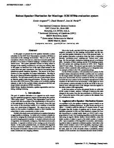
Figure 2.2: Example of speaker model adaptation.

¯ based on a given model λ 1977]. The EM iteratively estimate new model parameters λ ¯ ≥ p(X|λ). such that p(X|λ) The parameters of a GMM can also be estimated using Maximum A Posteriori (MAP) estimation, in addition to the EM algorithm. The MAP estimation technique derives a speaker model by adapting from a universal background model (UBM). The “Expectation” step of EM and MAP are the same. MAP adapts the new sufficient statistics by combining them with old statistics from the prior mixture parameters. Given a prior model and training vectors from the desired class, X = x1 ..., xT , we first determine the probabilistic alignment of the training vectors into the prior mixture components. For mixture i in the prior model P r(i|xt , λU BM ) is computed as the percentage of the mixture component i to the total likelihood, wi g(xt |µi , Σi ) P r(i|xt , λU BM ) = PM i=1 wi g(xt |µi , Σi )

(2.3)

Then, the sufficient statistics for the weight, mean and variance parameters is computed as follows:

ni =

T X

P r(i|xt , λprior ) weight

(2.4)

T 1 X P r(i|xt , λprior )xt mean ni

(2.5)

t=1

Ei (x) =

t=1

20


T 1 X P r(i|xt , λprior )x2t variance Ei (x ) = ni 2

(2.6)

t=1

Finally, the new sufficient statistics from the training data are used to update the prior sufficient statistics for mixture i to create the adapted mixture weight, mean and variance for mixture i as follows:

wi = [αiw ni /T + (1 − αiw )wi ]γ

(2.7)

µi = αim Ei (x) + (1 − αim )µi

(2.8)

µ2i = αiv Ei (x2 ) + (1 − αiv )(σi2 + µ2i ) − µ2i

(2.9)

The adaptation coefficients controlling the balance between old and new estimates are {αiw , αim , αiv } for the weights, means and variances, respectively. The scale factor, γ, is computed over all adapted mixture weights to ensure they sum to unity.

2.4.2

i-Vector

Different approaches have been developed recently to improve the performance of speaker recognition systems. The most popular ones were based on GMM-UBM. The Joint Factor Analysis (JFA) [Kenny et al., 2008] is then built on the success of the GMMUBM approach. JFA modeling defines two distinct spaces: the speaker space defined by the eigenvoice matrix and the channel space represented by the eigen-channel matrix. In [Dehak, 2009], it is proved that channel factors estimated using JFA, which are supposed to model only channel effects, also contain information about speakers. A new speaker verification system has been proposed using factor analysis as a feature extractor that defines only a single space, instead of two separate spaces [Dehak et al., 2011]. In this new space, a given speech recording is represented by a new vector, called total factors as it contains the speaker and channel variabilities simultaneously. Speaker recognition based on the i-vector framework [Dehak et al., 2011] is currently the state-of-the-art in the field. It is also reported in [Kenny et al., 2010,Franco-Pedroso et al., 2010,Shum et al., 2011,Shum et al., 2012,Vaquero Avilés-Casco, 2011,Senoussaoui et al., 2013] that i-vector features can also be successfully used in speaker diarization experiments. It is also shown in [Silovsky and Prazak, 2012] that modeling the speech


21

segments by i-vector and using cosine distance scoring improves the performance of a baseline speaker diarization system more that GMM based BIC clustering technique. Given an utterance, the speaker and channel dependent GMM supervector is defined as follows: M = m + Tw

(2.10)

where m is a speaker and channel independent supervector, T is a rectangular matrix of low rank and w is a random vector having a standard normal distribution N (0,1). The components of the vector w are the total factors. These new vectors are called i-vectors. M is assumed to be normally distributed with mean vector and covariance matrix TT t . The total factor is a hidden variable, which can be defined by its posterior distribution conditioned to the Baum–Welch statistics for a given utterance. This posterior distribution is a Gaussian distribution and the mean of this distribution corresponds exactly to i-vector. The Baum–Welch statistics are extracted using the UBM. Given a sequence of L frames {y1 , y2 , ......, yn } and a UBM Ω composed of C mixture components defined in some feature space of dimension F, the Baum–Welch statistics needed to estimate the i-vector for a given speech utterance u is given by :

Nc =

L X

P (c|yt , Ω)

(2.11)

P (c|yt , Ω)yt

(2.12)

t=1

Fc =

L X t=1

where c = 1, ...., C is the Gaussian index and P (c|yt , Ω) corresponds to the posterior probability of mixture component c generating the vector yt . The centralized first-order Baum–Welch statistics has also to be computed for the extraction of i-vectors as follows:

Fˆc =

L X

P (c|yt , Ω)(yt − mc )

(2.13)

t=1

where mc is the mean of UBM mixture component c. The i-vector for a given utterance can be obtained using the following equation:

w = (I + T t Σ−1 N (u)T )−1 . T t Σ−1 Fˆ (u)

(2.14)

22


where Nu is a diagonal matrix of dimension CF ×CF whose diagonal blocks are Nc I(c = 1, ......, C) . The supervector obtained by concatenating all first-order Baum–Welch statistics Fc for a given utterance u is represented by Fˆ (u) which has CF × 1 dimension. The diagonal covariance matrix, Σ , with dimension CF × CF estimated during factor analysis training models the residual variability not captured by the total variability matrix T . A clear and concise process of extraction of i-vectors is found in [Dehak et al., 2011]. After the extraction of raw i-vectors, normalization needs to be carried out on the raw i-vector to remove any useless information [Bousquet et al., 2011, Garcia-Romero and Espy-Wilson, 2011]. The normalization methods can be carried out at the feature or score level. One of the most widely used feature normalization techniques of i-vectors is length normalization [Bousquet et al., 2011, Garcia-Romero and Espy-Wilson, 2011]. Length normalization ensures that the distribution of i-vectors matches the Gaussian normal distribution and makes the distributions of i-vector more similar. It is also reported in [Jiang et al., 2012] that performing whitening before length normalization improves the performance of speaker verification systems. It is also reported in [Garcia-Romero and Espy-Wilson, 2011] that i-vector normalization improves the gaussianity of the ivectors. It reduces the gap between the underlying assumptions of the data and real distributions. It also reduces the dataset shift between development and test i-vectors. 1

w←

Σ− 2 (w − µ) 1

||Σ− 2 (w − µ)||

(2.15)

where µ and Σ are the mean and the covariance matrix of a training corpus, respectively. The data is standardized according to covariance matrix Σ and length-normalized (i.e., the i-vectors are confined to the hypersphere of unit radius). The two most widely and common intersession compensation techniques of i-vectors are Within-Class Covariance Normalization (WCCN) and Linear Discriminant Analysis (LDA). WCCN uses the within-class covariance matrix to normalize the cosine kernel functions in order to compensate for intersession variability [Dehak et al., 2011]. LDA attempts to define a reduced special axes that minimize the within-speaker variability caused by channel effects, and maximize between-speaker variability. It is shown in [Dehak et al., 2011,Dehak et al., 2010] that cosine kernel function is an effective classifier to categorize i-vectors. Cosine Distance


23

Figure 2.3: The i-vector extraction process.

Once the i-vectors are extracted from the outputs of speech clusters, cosine distance scoring tests the hypothesis if two i-vectors belong to the same speaker or different speakers. Given two i-vectors, the cosine distance among them is calculated as follows:

cos(wi , wj ) =

wi .wj Rθ ||wi ||.||wj ||

(2.16)

where θ is the threshold value, and cos(wi ,wj ) is the cosine distance score between clusters i and j. The corresponding i-vectors extracted for clusters i and j are represented by wi and wj , respectively. The cosine distance scoring considers only the angle between two i-vectors, not their magnitude. Since the non-speaker information such as session and channel variabilities affect the i-vector magnitude, removing the magnitudes can increase the robustness of i-vector systems [Dehak et al., 2010]. Probabilistic Linear Discriminant Analysis The i-vector representation followed by probabilistic linear discriminant analysis (PLDA) modeling technique is the state-of-the-art in speaker verification systems [Prince and Elder, 2007]. In speaker diarization, each i-vector represents the speech of one speaker. Speaker diarization needs to determine if two i-vectors belong to the same or different speakers.

24


PLDA has been successfully applied in speaker recognition experiments [Brummer et al., 2010]. It is also applied in [Jiang et al., 2012] to handle speaker and session variability in speaker verification task. It has also been successfully applied in speaker clustering since it can separate speaker and noise specific parts of an audio signal which is essential for speaker diarization [Prazak and Silovsky, 2011]. PLDA has also been successfully used in speaker clustering experiments and it is shown in the work of [Prazak and Silovsky, 2011] that PLDA-based clustering provides significance performance improvement than BICbased speaker clustering methods. It is also shown that PLDA scoring provides better speaker clustering performance than cosine scoring [Sell and Garcia-Romero, 2014].

Figure 2.4: Example of PLDA Model

In PLDA, assuming that the training data consists of J i-vectors where each of these i-vectors belong to speaker I, the j’th i-vector of the I’th speaker is denoted by:

wij = µ + F hi + Gwij + Σij

(2.17)

where µ is the overall speaker and segment independent mean of the i-vectors in the training dataset, columns of the matrix F define the between-speaker variability and columns of the matrix G define the basis for the within-speaker variability subspace. Σij represents any unexplained data variation. The components of the vector hi are the eigenvoice factor loadings and components of the vector wij are the eigen-channel factor loadings. The term F hi depends only on the identity of the speaker, not on the particular segment. Although the PLDA model assumes Gaussian behavior, there is empirical evidence that channel- and speaker- effects result in i-vectors that are non-Gaussian. It is reported in [Kenny, 2010] that the use of Student’s t-distribution, on the assumed Gaussian PLDA model, improves the performance. Since this normalization technique is complicated, a non-linear transformation of i-vectors called radial Gaussianization has been proposed


25

in [Garcia-Romero and Espy-Wilson, 2011]. It whitens the i-vectors and performs length normalization. This restores the Gaussian assumptions of the PLDA model. A variant of PLDA model called Gaussian PLDA (GPLDA) is shown to provide better results in [Garcia-Romero and Espy-Wilson, 2011]. Because of its low computational requirements, and its performance, it is the most widely used PLDA modeling. In GPLDA model, the within-speaker variability is modeled by a full covariance residual term which allows us to omit the channel subspace. The generative PLDA model for the i-vector is represented by

(2.18)

wij = µ + F hi + Σij

The residual term representing the within-speaker variability is assumed to have a normal distribution with full covariance matrix Σij . A special case of the simplified PLDA model where the speaker factors S is full-rank is termed as the two-covariance model in [Br¨ ummer and De Villiers, 2010, Cumani et al., 2013]. Given two i-vectors w1 and w2 , the PLDA computes the likelihood ratio of the two i-vectors as follows:

Score(w1 , w2 ) =

p(w1 , w2 |H1 ) p(w1 |H2 )p(w2 |H2 )

(2.19)

where the hypothesis H1 indicates that both i-vectors belong to the same speaker and H0 indicates they belong to two different speakers.

log(w1 , w2 ) = logN

" # " # " w1 µ Σ + SS T , ; w2 µ SS T

SS T Σ + SS T

#! −

logN (w1 ; µ, Σ + SS T ) − logN (w2 ; µ, Σ + SS T ) (2.20)

After straightforward algebra, this turns out to be,

log(w1 , w2 ) =

h

w1T

w2T

" i Σ + SS T SS T

SS T

#−1

h w1T

i h w2T − w1T w1T

i w2T −

Σ + SS T h i−1 h i−1 T T T T w1 Σ + SS w1 − w2 Σ + SS wt + C (2.21)

26


where all the constant terms have been incorporated into C, and can be omitted for a given PLDA model.

2.4.3

Speaker Factors

Given a UBM, a low rank eigenvoice matrix V that describes the speaker variability, and the supervector mn , the speaker factor xn is extracted as follows:

mn = mU BM + Vxn

(2.22)

The process of extracting speaker factors is similar to the i-vector extraction technique outlined in Section 2.4.2. The UBM training is the same both in the i-vector and speaker factor extraction techniques. The main difference is in the training of Total variability and eigenvoice matrices. While all the recordings of a given speaker are considered to belong to the same person in eigenvoice training, they are considered as being produced by different speakers in total variability matrix training.

Figure 2.5: Speaker factor extraction process. The difference between i-vector and speaker factor extraction is the training of the total variability and eigenvoice matrix.

Once the speaker factors are extracted, there are different scoring techniques to check similarity of speaker factors . The most widely used scoring technique is the cosine distance and Mahalanobi distance. Speaker factors have been successfully used for speaker segmentation in [Desplanques et al., 2016]. The speaker factors have been extracted on a frame-by-frame basis using an

2.4. Speaker Modeling Techniques Input layer

27 Hidden layer

Output layer

Input 1 Input 2 Output Input 3 Input 4

Figure 2.6: Example of Artificial Neural Network.

eigenvoice matrix and the Mahalanobis distance is applied on speaker factors to generate speaker boundaries. The work in [Desplanques et al., 2016] shows that the use of speaker factors provides better DER result more than the BIC segmentation technique.

2.4.4

Artificial Neural Networks

Artificial neural networks (ANNs) have recently been used in different speech applications. Feed-forward neural networks which moves forward (from the input nodes to output nodes through the hidden nodes) have been used. A feed-forward neural network is created for each speaker. Each network contains one output trained to be active only for this speaker. During testing, a feature vector is fed forward through each network, and the identification is determined by the network with the highest accumulated output values. Artificial neural network (ANNs) have recently been applied successfully in speaker diarization tasks as reported in [Yella et al., 2014]. Three different neural networks have been trained in [Yella et al., 2014] which are used to generate features for speaker diarization. The first network is to decide if two speech segments belong to the same or different speakers. The second network is trained to classify a given speech segment into a predetermined set of speakers. The third network is an auto-encoder which is trained to reconstruct the input at the output layer with as low reconstruction error as possible. It is reported in [Yella et al., 2014] that the hidden layers of networks trained transform spectral features into a space more conducive to speaker discrimination.

28

2.4.5


Deep Neural Networks

A deep neural network (DNN) is a feed-forward, artificial neural network that has more than one layer of hidden units between its inputs and its outputs [Hinton et al., 2012]. Each hidden unit, j, typically uses the logistic function to map its total input from the layer below, xj , to the scalar state, yj that it sends to the layer above.

yj = logistic(xj ) =

1 , 1 + e−xj

xj =

X

yi wij

(2.23)

i

where bj is the bias of unit j, i is an index over units in the layer below, and wij is the weight on a connection to unit j from unit i in the layer below. For multiclass classification, output unit j converts its total input, xj , into a class probability, pj , by using the softmax non-linearity as follows:

exp(xj ) pj = P k exp(xk )

(2.24)

where k is an index over all classes. DNN’s can be discriminatively trained by backpropagating the derivatives of a cost function to calculate the difference between the target outputs and the actual output [Rumelhart et al., 1988]. When using the softmax output function, the natural cost function C is the cross-entropy between the target probabilities d and the outputs of the softmax, p:

C=

X

dj log pj

(2.25)

j

where the target probabilities are the supervised information provided to train the DNN classifier. When training large data sets, it is efficient to compute the derivatives on a small, random mini-batch of training data sets, rather than the whole training set, before updating the weights in proportion to the gradient. This stochastic gradient descent method can be further improved by using a momentum coefficient that smooths the gradient computed for each mini-batch. One of the main problem in DNN is overfitting. To overcome the problem of overfitting, a penalty term can be applied on large weights proportional to their squared magnitude.

2.5. Speaker Segmentation

29

The learning can also be stopped at a point where performance on a test data set starts getting worse [Bourlard and Morgan, 2012]. When the number of hidden layers and the units per layer is increased, the DNN becomes more flexible to model very complex and highly non-linear relationships between inputs and outputs. Although this is good for high-quality acoustic modeling, it may also lead to the overfitting. DNNs are currently widely applied in audio, image and speech processing applications [Ciregan et al., 2012,Lee et al., 2009,Mohamed et al., 2012,Dahl et al., 2012,Arisoy et al., 2012,Stafylakis et al., 2012]. It is reported in [Mohamed et al., 2012,Hinton et al., 2012, Yao et al., 2012] that DNNs provide better results when they are used as acoustic modeling in speech recognition. DNNs have also been used in speaker recognition experiments successfully in [Ghahabi and Hernando, 2014]. They have also been successfully used in different stages of speaker diarization: feature extraction [Yella and Stolcke, 2015], speaker segmentation and speaker clustering [Jothilakshmi et al., 2009]. Speaker Separation Deep Neural Network has also been used in [Yella and Stolcke, 2015] to extract features from the bottleneck layer and classify speakers.

2.5

Speaker Segmentation

Speaker segmentation finds points in the audio stream which are likely to be the change points between speakers. According to [Chen and Gopalakrishnan, 1998], the three major methods to perform speaker segmentation are: Silence based methods These methods assume that a silence occurs between utterances of two speakers. They are normally dependent on the threshold values of the short term energy. However, these methods provide poor results [Kemp et al., 2000]. There are two main categories in this method. These are energy based and decoder based systems. The energy based systems use energy detector to find the silence segments [Kemp et al., 2000]. The decoder based systems use a full recognition system to find change points from detected silence locations [Kubala et al., 1997]. However, there is no clear relationship between the existence of silence in a recording and change of speaker. Therefore, these methods are not widely used in speaker diarization. Model based methods

30


These methods train different speaker classes and derive different speaker models for a closed set of acoustic classes such as telephone or wide-band, male or female, music, speech or silence using training corpus. Then, the audio signal is classified using maximum likelihood techniques [Gauvain et al., 1999]. The boundaries between the models will be the segmentation change points. However, model based methods have a robustness problem as they do not generalize for unseen data. Metric based method These methods are the most common and wdiely used segmentation techniques [Ajmera and Wooters, 2003]. Metric based methods do not require any prior knowledge about the number of speakers and signal characteristics.They use distance metric between every two contiguous speech segments as a decision measure to determine change points [Sinha et al., 2005, Siegler et al., 1997]. The metric based method tests two hypothesis: The first hypothesis, H1 , assumes that the two contiguous speech segments belong to the same speaker and is described by a single model. The second hypothesis, H2 assumes that the two contiguous speech segments belong to different speakers and are described by different models. The distance metric is compared to a threshold in order to select one of the two hypothesis.

• Bayesian Information Criterion (BIC) It is used to evaluate whether a change point occurs between two consecutive speech segments. Two BIC values, H1 and H2 , are computed. Let us consider to model Xi with d dimensional feature vectors. Assuming that the two contiguous speech segment analysis windows X and Y are located around time Tj, we need to find whether a speaker change point occurs at Tj or not. Let Z = X ∪ Y , the problem is formulated as a statistical test between the two hypotheses. In the case of H1 , there is no speaker change point at time Tj. The log likelihood H1 is obtained as follows:

H1 =

nx X i=1

log p(Xi |θz ) +

ny X

log p(Yi |θz )

(2.26)

i=1

where nx and ny are the number of frames in speech segments X and Y, respectively. Speech segments X and Y are are modeled by θz in H1 . In the case of H2 , a speaker change point exists at time Tj . The speech segments X and Y are modeled by two speaker models, which are represented by θx and θy , respectively. Then, the log likelihood H2 is obtained as follows:

2.5. Speaker Segmentation

31

Figure 2.7: Example of audio signal with three speakers.

H2 =

nx X

log p(Xi |θx ) +

i=1

ny X

log p(Yi |θy )

(2.27)

i=1

The dissimilarity between the two speech segments, X and Y, is estimated by using BIC criterion defined as:

∆BIC = H2 − H1 −

d + (d + 1) λ (d + ) log nz 2 2

(2.28)

where nz is the number of frames in analysis window Z (i.e., nz = nX + nY ) and λ is a penalty factor. If BIC is greater than 0, there is a speaker change point between the two contiguous speech segments. Otherwise, there is no a speaker change point between the two contiguous speech segments. It is reported in [Zhou and Hansen, 2005] that the choice of the analysis window size in BIC computation should be carefully selected. If it is too large, it may yield a high number of miss detections. If it is too short, it causes poor model estimation and poor segmentation accuracy. The penalty factor was introduced to adjust the penalty effect on the comparison of two adjacent windows that may have different window lengths. Although BIC is computationally more intensive than other metric methods, its good performance has kept it as the algorithm of choice in speaker diarization.

32


Figure 2.8: Example of ∆ BIC Values.

• Generalized Likelihood Ratio(GLR) GLR has been proposed as a metric for change detection in [Willsky and Jones, 1976]. Given sequences of feature vectors Xi and Xj from two contiguous speech segments i and j, respectively, GLR is calculated as a likelihood ratio under the assumption of H1 and H2 . Therefore, two different speaker models are generated for H1 and H2 . In H1 , θi,j is estimated with Xi and Xj . In H2 , two models are estimated: θi from Xi, and θj from Xj. The GLR is then computed as follows:

GLR(

L(Xi,j |θi,j ) H1 )= H2 L(Xi |θi )L(Xj |θj )

(2.29)

where L is the likelihood. A high value of GLR shows that the two speech segments are modeled by a single model and a low value of GLR shows that the two speech segments are modeled by two models. GLR can be used together with BIC in a two step speaker segmentation process [Delacourt and Wellekens, 2000]. In the first step, the most likely speaker change points are detected by GLR and, in the second step, BIC is used to refine the speaker change points.

• Gish Distance It is a likelihood based metric obtained as a variation to the GLR. It is defined as:

2.6. Speaker Clustering

DGish (i, j) =

33

|Si |α |Sj |(1−α) −N log( ) 2 |αSi + (1 − α)Sj |

where Si and Sj are the covariance matrices of segments i and j and α =

(2.30) Ni Ni +Nj .

• Information Change Rate (ICR) Information Change Rate (ICR): It is another distance measure that is recently introduced for speaker diarization [Vijayasenan et al., 2007, Vijayasenan et al., 2009, Han and Narayanan, 2008]. ICR can be used to delineate the similarity of two speech speech segments determining the variation in terms of information that would be obtained by merging them. ICR similarity is not based on model of speech segments. It is based on the distance between the segments in a space of relevance variables with maximum mutual information or minimum entropy. ICR is computationally efficient and more robust to data source variation more than BIC distance [Han and Narayanan, 2008]. The results of speaker segmentation may contain two types of error. The first type of error occurs when a true segment boundary is not detected (i.e., deletion). The second type of error occurs when a segmented boundary does not correspond to the true segment boundary in the reference (i.e., false alarm).

2.6

Speaker Clustering

Speaker clustering groups speech segments that belong to a particular speaker. It has two major categories based on its processing requirements. Its two main categories are online and offline speaker clustering. In the former, speech segments are merged or split in consecutive iterations until the optimum number of speakers is acquired. Since the entire speech file is available before decision making in the later, it provides better results more than the online speaker clustering. The most widely used and popular technique for speaker clustering is Agglomerative Hierarchical Clustering (AHC). AHC builds a hierarchy of clusters, that shows relations between speech segments, and merges speech segments based on similarity. AHC approaches can be classified into bottom-up and top-down clustering. Two items need to be defined in both bottom-up and top-down clustering: 1. A distance between speech segments to determine acoustic similarity. The distance metric is used to decide whether or not two clusters must be merged (bottom-up clustering) or split (top-down clustering).

34

Chapter 2. State-of-the-art in Speaker Diarization 2. A stopping criterion to determine when the optimal number of clusters (speakers) is reached.

• Bottom-up (Agglomerative): It starts from a large number of speech segments and merges the closest speech segments iteratively until a stopping criterion is met. This technique is the most widely used in speaker diarization since it is directly applied on the output of speech segments from speaker segmentation. A matrix of distances between every possible pair of clusters is computed and the pair with highest BIC value is merged. Then, the merged clusters are removed from the distance matrix. Finally, the distance matrix table is updated using the distances between the new merged cluster and all remaining clusters. This process is done iteratively until the stopping criterion is met or all pairs have a BIC value less than zero . The bottom-up approach has been used for many years in pattern classification in [Duda and Hart, 1973] but was first considered for speaker clustering in [Duda et al., 2001] and [Siegler et al., 1997]. A two pass speaker clustering has been proposed in [Chen and Gopalakrishnan, 1998]. In the first pass, the speech data is equally segmented using GLR distance matrix with agglomerative clustering until the desired number of speakers is reached. The second pass trains speaker models and iteratively decodes and trains speaker models until the total likelihood converges.

• Top-down: Top-down Hierarchical Clustering methods start from a small number of clusters, usually a single cluster, that contains several speech segments, and the initial clusters are split iteratively until a stopping criterion is met. It is not as widely used as the bottom-up clustering.

Figure 2.9: Bottom-Up and Top-down approaches to clustering

2.7. Approaches to Speaker Diarization System

2.7

35

Approaches to Speaker Diarization System

This section describes some of the state-of-the-art speaker diarization systems. The HMM/GMM based system provides the the state-of-the-art in NIST-RT [National Institute of Standards and Technology, 2003] evaluation campaigns. The information bottleneck framework provides comparable results to that of HMM/GMM based system [Vijayasenan and Valente, 2012]. HMM/GMM system In HMM/GMM based speaker diarization system, each speaker is represented by a state of an HMM and the state emission probabilities are modeled using GMMs. The initial clustering is performed initially by partitioning the audio signal equally which generates a set of segments {si }. Let ci represent ith speaker cluster, bi represent the emission probability of cluster ci and ft denote a given feature vector at time t. Then, the log-likelihood logbi (st ) of the feature ft for cluster ci is calculated as follows:

logbi (st ) = log

X

(r)

(r)

(r)

wi N (fi , µi , Σi )

(2.31)

(r)

(r)

(r)

(r)

where N () is a Gaussian pdf and wi , µi , Σi matrices of the

rth

are the weights, means and covariance

Gaussian mixture component of cluster ci , respectively.

The agglomerative hierarchical clustering starts by overestimating the number of clusters. At each iteration, the clusters that are most similar are merged based on the BIC distance. The distance measure is based on modified delta Bayesian information criterion [Ajmera and Wooters, 2003]. The modified BIC distance does not take into account the penalty term that corresponds to the number of free parameters of a multivariate Gaussian distribution and is expressed as:

∆BIC(ci , cj ) =

X

logbij (ft ) −

ft ∈{ci ∪cj }

X ft ∈ci

logbi (ft ) −

X

logbj (ft )

(2.32)

ft ∈cj

where bij is the probability distribution of the combined clusters ci and cj . The clusters that produce the highest B IC score are merged at each iteration. A minimum duration of speech segments is normally constrained for each class to prevent decoding shortsegments. The number of clusters is reduced at each iteration. When the maximum ∆BIC distance among these clusters is less than threshold value 0, the speaker diarization system stops and outputs the hypothesis. Information bottleneck (IB) system

36


Information Bottleneck (IB) system is a non-parametric system based on information theoretic principles. Its results are comparable with the HMM/GMM system [Wooters and Huijbregts, 2008]. The main advantage of IB is it requires less computation time more than HMM/GMM systems [Vijayasenan et al., 2009, Vijayasenan and Valente, 2012]. IB clustering clusters segments with similar distributions over a set of variables called relevance variables. Let X = {x1 , x2 , ..., xn } represent the input variables to be clustered and Y = {y1 , y2 , ..., ym } denote the relevance variables with meaningful information about clustering output C = {c1 , c2 , ..., cr }. IB method tries to optimize the clustering process by maximizing the following equation:

F = I(Y, C) −

1 I(C, X) β

(2.33)

where β is a Lagrange multiplier, I(X, C) denotes the mutual information where X represents the speech segment set at each iteration and C represents the clusters, and I(Y, C) measures the mutual dependence between the relevant variables Y and the clustering partition C. The IB system uses a greedy technique to optimize the clustering process [Vijayasenan and Valente, 2012]. It starts with unique segmentation where each segment is considered as a set of input variables X. The set of relevance variables Y is components of background GMM estimated from the speech segments. Given input speech segment xi , the posterior distribution of the relevance variables for the segment xi is obtained using Bayes rule. The clustering of IB is initialized with each member of the set of speech segment X and the two clusters with the most similar distribution are merged at each iteration. Other approaches The HMM/GMM and IB based speaker diarization systems are based on an agglomerative clustering framework. There are also other approaches to speaker diarization. They are described as follows: Top down system The top down-approach starts by modeling the entire audio signal with a single speaker model. Then, it successively generates new speaker models. The generation of new speaker models can be done using some criterion such as duration of the speech segment. A new speaker model is generated for these speech segments. This process is performed iteratively until the final number of speaker is found. Top-down approaches are not

2.8. Evaluation Metrics

37

widely used as the bottom up one. They are however computationally efficient and their performance can be improved using cluster purification as reported in [Bozonnet et al., ]. Factor analysis techniques Factor analysis techniques which are the state of the art in speaker recognition have recently been successfully used in speaker diarization [Kenny et al., 2010,Franco-Pedroso et al., 2010, Shum et al., 2011]. The speech clusters are first represented by i-vectors and the successive clustering stages are performed based on i-vector modeling. The use of factor analysis technique to model speech segments reduces the dimension of the feature vector by retaining most of the relevant information. Once the speech clusters are represented by i-vectors, cosine-distance and PLDA scoring techniques can be applied to decide if two clusters belong to the same or different speaker(s). [Dehak et al., 2011].

2.8

Evaluation Metrics

Diarization Error Rate (DER) is the metric used to measure the performance of speaker diarzation systems as described and used by NIST in the RT evaluations (NIST Fall Rich Transcription on meetings 2006 Evaluation Plan 2006). It is measured as the fraction of time that is not attributed correctly to a speaker or non-speech. A script named MD-eval-v12.pl has been used in the experiments. When DER is calculated, the hypothesized diarization output does not need to identify the speakers by name or definite ID. The speaker name or speaker id should not be the same in the hypothesis and the reference segmentation. The evaluation script first does an optimum one-to-one mapping of all speaker label ID between hypothesis and reference files. This allows the scoring of different ID tags between the two files. When evaluating DER, NIST uses a collar of 250 ms at the beginning and end of each segment boundary not to penalize slight discrepancies in the start and end times of the speech segments. The DER is calculated as follows: PS DER =

s=1 dur(s).(max(Nref (s), Nhyp (s)) PS s=1 dur(s).Nref

− Ncorrect (s))

(2.34)

where S is the total number of speaker segments where both reference and hypothesis files contain the same speaker pairs. Nref (s) and Nsys (s) represent the number of speaker speaking in segment s. The number of speakers that speak in segment s and are correctly

38


matched between reference and hypothesis is represented by Ncorrect (s). The duration of segment s is represented by dur(s). The DER is composed of the following three errors:

• Speaker Error: It is the percentage of scored time that a speaker ID is assigned to the wrong speaker. Speaker error is mainly a diarization system error (i.e., it is not related to speech/non-speech detection.) It also does not take into account the overlap speeches not detected.

PS Speaker Error =

s=1 dur(s).(min(Nref (s), Nhyp (s)) PS s=1 dur(s).Nref

− Ncorrect (s))

(2.35)

• False Alarm: It is the percentage of scored time that a hypothesized speaker is labelled as a non-speech in the reference. The false alarm error occurs mainly due to the the speech/non-speech detection error (i.e., the speech/non-speech detection considers a non-speech segment as a speech segment). Hence, false alarm error is not related to segmentation and clustering errors.

PS F alse Alarm =

s=1 dur(s).(Nhyp (s)) − Nref (s)) PS s=1 dur(s).Nref

(2.36)

• Missed Speech: It is the percentage of scored time that a hypothesized non-speech segment corresponds to a reference speaker segment. The missed speech occurs mainly due to the the speech/non-speech detection error (i.e., the speech segment is considered as a non-speech segment). Hence, missed speech is not related to segmentation and clustering errors.

PS M iss Speech =

s=1 dur(s).(Nref (s)) − Nhyp (s)) PS s=1 dur(s).Nref

(2.37)

• Overlap Error: When there are multiple speakers in the speech segment, the speaker diarization system has to detect and assign the segment to to all speakers. Therefore, overlap error is the percentage of scored time that some of the multiple speakers in a segment are not assigned to any speaker. The overlap error falls into one the three types of the previously mentioned diarization errors: speaker error when a speaker is detected to be present in the speech segment but the speaker is

2.8. Evaluation Metrics

39

not actually present, false alarm speech if more number of speakers are detected than the actual number of speakers in the overlapped speech segment, and missed speech when fewer speakers are detected than the actual number of speakers in the segment.

Therefore, the total DER is calculated as: DER = Speaker Error + F alse Alarm + M iss Speech + Overlap Error

(2.38)

Once the DER is calculated for each show, the time weighted average is calculated among all meetings to find average DER for given set of shows. It is usual to score the diarization error rate ignoring the overlapped speech segment.

Chapter 3

The UPC Baseline Speaker Diarization System This chapter describes the techniques and implementation of the baseline speaker diarization of UPC which we use as a benchmark for the proposed systems. The baseline speaker diarization system is based on HMM/GMM systems and uses MelFrequency Cepstral Coefficients (MFCC). It uses a bottom-up agglomerative clustering approach that uses a modified version of the BIC distance in order to iteratively merge the closest clusters. Each HMM state represents a speaker whose emission probabilities are modeled using GMM. The baseline speaker diarization system follows multiple steps of agglomerative clustering and realignment (i.e., the speaker segmentation and clustering are carried out iteratively). The system is initialized first with many number of speakers. Then, the two most similar clusters are merged at each iteration. After merging, the time boundaries of segments are realigned using a Viterbi segmentation. The process is iteratively repeated until a stopping criterion is met. A detailed description about the baseline system used in the thesis is found in [Luque, 2012]. As it is shown in Figure 3.1, the baseline speaker diarization system consists of three modules. These are the feature extraction, speaker segmentation and speaker clustering. The three main stages of the baseline system diarization are as follows: • Feature extraction and removal of non-speech frames. A uniform initial clustering is performed by partitioning the data equally (see Fig. 3.1, block A). • Model complexity selection based on the amount of data per cluster and the cluster complexity ratio (CCR) is carried out to fix the amount of speech (seconds) per 41

42

Chapter 3. The UPC Baseline Speaker Diarization System Gaussian. An HMM/GMM training and cluster realignment is carried out using by Viterbi decoding by taking the maximum likelihood scores (Fig. 3.1 block B). • Agglomerative clustering is carried out using Bayesian information criterion (BIC) metric among clusters. A threshold value is used to stop the speaker diarization system and output the final hypothesis (Fig. 3.1 block C).

The rest of this paper is organized as follows. Section 3.1 describes the front-end Processing technique used in the baseline system. The Cluster Initialization technique is discussed Section 3.2. The speaker segmentation and clustering techniques are outlined in Section 3.3 and Section 3.4. Finally, the merge and stopping criterion are discussed in section 3.5.

Figure 3.1: The UPC baseline speaker diarization system architecture.

3.1

Front-end Processing

The speech parameterization of the baseline system is based on a short-term estimation of the spectrum energy in several sub-bands. The speech channel is analyzed in frames

3.2. Cluster Initialization

43

of 30 milliseconds at intervals of 10 milliseconds and 16 kHz of sampling frequency. Each frame window is processed subtracting the mean amplitude from each sample. A Hamming window was applied to each frame and a FFT computed. The FFT amplitudes were then averaged through overlapped triangular filters, with central frequencies and bandwidths defined according to the Mel scale.

Speech/Non-Speech Detection Technique Manually annotated speech references (Oracle SAD) have been employed to extract the speech frames and discard non-speech regions. Since speech references have been used, the percentage of false alarms and missed speech have zero values in the experimental results. Hence, DER values reported in the following sections corresponds purely to speaker time confusion produced by the diarization system.

Speech Features Mel Frequency Cepstral Coefficients (MFCC) have been used as acoustic features in the baseline speaker diarization system. They are computed with the aid of a psychoacoustically motivated filterbank, followed by logarithmic compression and discrete cosine transform (DCT). The dimensions of MFCCs is 20. The MFCC are used without the ∆ and ∆∆ parameters.

3.2

Cluster Initialization

First, the speech signal is equally partitioned as it is shown in (Fig. 3.1 block A) which generates the initial clusters. The initial number of clusters depends on meeting duration but it is constrained in the range [10, 65] clusters. This methods enables to deal with common issues of AHC such as over-clustering and high computational cost due to combinatorial explosion in pair-wise distance computation. A method to reduce manual tuning of these values is also implemented. This reduces the sensitivity of the initialization values and therefore reduces the need for manual tuning significantly. At the same, it also increases the accuracy of the system. The Initial number of clusters is calculated as follows: Kinit =

N , Ginit RCC

(3.1)

44

Chapter 3. The UPC Baseline Speaker Diarization System

where N stands for the number of total frames in a recording and Ginit is the number of Gaussians initially assigned to each cluster. The complexity ratio, RCC , stands for the minimum amount of speech data in frames needed per each Gaussian mixture in the cluster model. They are fixed to 5 Gaussians initially and 7 seconds per Gaussian, respectively. This method of cluster partitioning allows to build a ”pure” enough initial cluster segmentation which is a key point in AHC algorithm [Imseng and Friedland, 2010, Luque et al., 2008].

RCC = 0.01 × Y + 2.6

(3.2)

where RCC is the number of Gaussians per segment and Y is the amount of speech in second.

Automatic Model Complexity Selection At each iteration j, the number Mij of Gaussian mixtures to model the cluster i is updated using the following equation:

Mij =

h

Nij RCC

+ 0.5

i

(3.3)

where Nij is the number of frames belonging to the cluster i. After merging two segments, a new segment model is trained by pooling all the features from the merged segments and fixing the model complexity according to the RCC value. The automatic selection of the modeling complexity has been shown to provide a good performance and it avoids the use of the penalty term in the classical BIC metric computation [Anguera et al., 2006b]. After the initial segmentation is carried out, each cluster is modeled by mixture of Gaussians to fit the probability distribution of the features using the classical expectationmaximization (EM) algorithm. The baseline system first compared different values of seconds per Gaussian with their corresponding speaker error rates and tuned the seconds per Gaussian value. Hence, seconds per Gaussian values are dependent the duration of the speech data. If the speech segment is long, it has have more number of Gaussians. If the speech segment is short, it has have few number of Gaussians.

3.3. Iterative Viterbi-Segmentation

45

Figure 3.2: Ergodic HMM/GMM system with a minimum duration constraint. The minimum duration constraint of the baseline system that ensures the minimum length of the speaker turn duration. Each state is a subset of substates.

3.3

Iterative Viterbi-Segmentation

The baseline system models each set of clusters using ergodic hidden Markov model (HMM) where each state in the model represents one cluster. Give a set of speech segments {X1 , X2 , ......., Xn }, the baseline system finds the optimal number of clusters K and their corresponding acoustic models that produce the best segmentation using the following equation:

θk∗ , k ∗ = arg max{P r(X, pbest |θk , k)} θk ,k

(3.4)

where pbest is the Viterbi path with the highest likelihood (i.e., sequence of states that produce the maximum likelihood given the observations). After the completion of the algorithm execution, each remaining state is considered to represent a different speaker. This is done to refine the initial segmentation and improves the speaker boundaries [Tranter and Reynolds, 2006].

46


Figure 3.3: Example of minimum duration constraint.

We want to find a set of clusters and their acoustic models that maximize the likelihood of the data based on this HMM topology. Since we do not want to consider all possible values for k, a maximum value is selected for k using the initial segmentation outlined in Section 3.2. After each iteration of merging clusters, the value of k is reduced until we find an optimal number of clusters k ∗ and their acoustic models θk∗ . A minimum duration (MD) is also constrained on the HMM topology as it is shown in Figure 3.3. Each state of the HMM consists of a set of sub-states imposing a minimum duration for each model. Each one of the sub-states has a probability density function modeled via a Gaussian mixture model (GMM). The same GMM model is tied for all sub-states of a given state. After entering a state at time n, the model moves to the following sub-state with probability 1.0 until the last sub-state is reached. It can remain in the same sub-state with transition weight α, or jump to the first sub-state of another state with weight

β K

, where K is the number of active states at that time.

After merging of two clusters at each iteration, the the total number of parameters in the HMM decreases. The likelihood scores at each iteration reduce when the same amount of data is modeled using fewer parameters. Since the merging process decreases the likelihoods of equation 3.4, a threshold value to stop merging the process has to selected.

3.4

Speaker Clustering

Once the speech segments have been generated by Viterbi segmentation, the speaker clustering merges the speech of the same speakers iteratively. A single cluster is modeled for each speaker in the audio, and all speech parts of a specific speaker are represented in a single cluster. The baseline system is based on the most widely used agglomerative hierarchical clustering (AHC) technique. The speech segments generated by Viterbi segmentation are

3.4. Speaker Clustering

47

modeled by Gaussian mixtures, fitting the probability distribution of the features by the classical expectation-maximization (EM) algorithm. Segments which belong to the same speaker are represented in a single model. The minimum duration of speaker segment is restricted to 3 seconds as in [Ajmera and Wooters, 2003]. The selection of 3 second as a minimum duration in the baseline system is also justified in [Luque, 2012] (see Figue 3.4). The figure shows that the selection of 3 provides the best DER among different minimum duration values.

Figure 3.4: DER results on NIST Transcription 2006 and 2007 evaluation conference data using the minimum duration into account in the HMM decoding.

The figure is taken from thesis of [Luque, 2012] (baseline system) on page number 167. The clustering technique groups acoustically similar segments based on the Bayesian information criterion (BIC) metric among Gaussian distributions. At each iteration, the two segments with the highest BIC distance are merged. The HMM decoding process is repeated and a new mixture of Gaussians is assigned for the new set of clusters. The similarity matrix of the cluster pairs is updated. This procedure is iterated until the stopping criterion is met.The stopping criterion is met when the maximum BIC distance among all set of clusters is less than 0. Finally, the speaker diarization system outputs the hypothesis results (see Figure 3.1, block C). There are different ways of performing speaker segmentation and speaker clustering in speaker diarization. One of the method is performing segmentation first and running speaker clustering next. This method lacks flexibility since it doesn’t provide the option of correcting the speaker segmentation errors. The other method is performing the speaker segmentation and speaker clustering together iteratively. This method enables to refine the speaker segmentation errors. The UPC baseline system uses the second method. It uses an iterative bottom-up strategy based on HMM alignments and BIC values. Segments that belong to the same speaker are combined in a new model at

48


each iteration. A time constraint is imposed as in [Ajmera and Wooters, 2003] on the duration of the speaker segments through a hierarchical modeling of each state as it is shown in Figure 3.3. The Viterbi decoding decisions are based on the estimation of the observation probabilities of accumulated likelihoods per cluster/state in a 3 seconds window. This procedure is carried out iteratively until the stopping criterion is reached. The stopping criterion is reached when the highest BIC distance scores among the set of clusters is less than 0. Finally, the system output the speaker segmentation outputs. Since the segmentation and clustering steps are performed iteratively in the baseline system, the errors made in the segmentation step are corrected in the clustering.

3.5

Merging and Stopping Criterion

One the speech segments have been generated by the Viterbi segmentation and each segment is assigned a cluster, the speaker clustering modules merges the two closest clusters. This process is performed iteratively until there are no more clusters to merge. This techniques requires two metrics: which pairs of clusters to merge at each iteration and when to stop merging. The UPC baseline speaker diarization system uses the modified BIC algorithm described in [Ajmera and Wooters, 2003] to merge clusters and stop merging. Given two speech segments X and Y , the modified BIC algorithm decides whether the speech segments X and Y are uttered by the same speaker (H1 ) or different speakers (H2 ). Let Z = X ∪ Y . The modified BIC equation is defined as follows:

∆BIC = BIC(X, Y ) = H1 − H2 ≶ 0

(3.5)

which does not take into account the penalty term that corresponds to the number of free parameters of a multivariate Gaussian distribution. While model H1 assumes that the speech segments are represented by the same speaker, model H2 assumes that the two speech segments belong to two different speakers. The log likelihood of H1 is obtained as follows:

H1 =

nx X i=1

log p(Xi |θz ) +

ny X

log p(Yi |θz )

(3.6)

i=1

where nx and ny are the number of frames in speech segments X and Y, respectively. Speech segments X and Y are are modeled by θz in H1 .

3.5. Merging and Stopping Criterion

49

In the case of H2 , a speaker change point exists at time Tj . The speech segments X and Y are modeled by two speaker models, which are represented by θx and θy , respectively. Then, the log likelihood H2 is obtained as follows:

H2 =

nx X i=1

log p(Xi |θx ) +

ny X

log p(Yi |θy )

(3.7)

i=1

If BIC (X,Y) is greater than 0, speech segment X and Y are modeled by one speaker model, θZ . If BIC(X,Y) is less than 0, speech segment X and Y are modeled by two different speaker models, θX and θY . Equation 3.5 is similar to traditional BIC criterion except it doesn’t use the penalty term. The number of parameters in model is equal to the sum of the number of parameters in θx and θy . The segmentation obtained from the outputs of the segmentation (see Figure 3.1) defines a new set of speaker clusters and has to be trained at each iteration. We look for the the set of BIC scores for clusters Y and Y satisfying BIC(X, Y ) ¿ 0. When there are many candidate pairs, we choose the pair of clusters with highest BIC score. This method provides a fully automatic stopping criterion that does not require the use of any tunable parameters. The stopping criterion for clustering is based on a threshold value of the BIC distances among all clusters. When the maximum BIC distance among these clusters is less than threshold value 0, the speaker diarization system stops and outputs the hypothesis.

Chapter 4

Long-term Speech Features for Speaker Diarization Feature extraction plays a significant role on the performance of speaker diarization systems. It needs to extract relevant information from the acoustic signal that can separate the different speaker present in the signal while discarding unwanted signals at the same time such as noise. It transforms raw acoustic signal into compact representation. It computes a sequence of feature vectors that represents compact speech signal. The feature vectors which are extracted from the raw signal emphasize speaker specific properties and suppress statistical redundancies. Although different types of features can be extracted from speech signals, only some of them can be used to discriminate speakers. According to [Kinnunen and Li, 2010], an ideal speech features have the following characteristics: they have large betweenspeaker variability and small within-speaker variability, they are robust against noise and distortion, they occur frequently and naturally in speech, they are easy to measure from speech signal, they are difficult to impersonate and they are not affected by the speaker’s health or long-term variations in voice. There are generally two broad categories of speech features. These are the short-term and long-term features. Short-term spectrum based features are the most widely used in speaker diarization systems since the short-term spectrum based features carry information about the vocal tract characteristics of individual speakers. They are also easy to extract and provide better performance. Short-term features are descriptors of the short-term spectral envelope which is an acoustic correlate of timbre and the resonance properties of the supralaryngeal vocal tract. 51

52

Chapter 4. Long-term Speech Features for Speaker Diarization

They are extracted from either the short-term Fourier transform of the windowed speech signal or from linear prediction (LP) analysis. They are typically extracted for every 10 ms from a window size of around 30 ms. Speech signal continuously vary because of articulatory movements. Therefore, it needs to be broken down into short frames of about 20-30 milliseconds duration [Kinnunen and Li, 2010]. The speech signal is quasi-stationary within this interval and feature vectors are extracted from each frame. Mel Frequency Cepstral Coefficients (MFCC) are the most widely used short-term acoustic features for speaker diarization [Anguera et al., 2012, Ajmera and Wooters, 2003]. They are computed with the aid of a psychoacoustically motivated filterbank, followed by logarithmic compression and discrete cosine transform (DCT). The dimensionality of MFCCs for speaker diarization is mostly around 20. Other widely used short-term spectral features used for speaker diarization include perceptual linear prediction coefficients (PLP) [Sinha et al., 2005], and linear prediction cepstral coefficients (LPCCs) [Ajmera and Wooters, 2003]. Although short-term spectral features are the most widely used speech features for different speech applications including speaker diarization, it is reported in [Friedland et al., 2009] that long-term features can be employed to reveal individual differences which can not be captured by short-term spectral features. Long-term speech features also have more discriminative power more than the short-term speech features. The selection of prosodic and other long-term features and their combination with MFCCs dramatically increases the accuracy of a state-of-the-art speaker diarization system [Friedland et al., 2009]. It is also reported in [Zelen´ ak and Hernando, 2011] the performance of the stateof-the-art speaker diarization systems can be improved by combining spectral features with prosodic features to detect overlap speeches in speaker diarization system. Long-term features are extracted from portions of speech longer than one frame unlike short-term features which are extracted from a single speech frame. Long-term features capture phonetic, prosodic, lexical, syntactic, semantic and pragmatic information. They are also robust to channel variation since lexical usage or temporal patterns do not change with the change of acoustic conditions [Shriberg, 2007]. The long-term speech features used in the experiments are the delta dynamic, voicequality, prosody and GNE features.

4.1. Dynamic Features

4.1

53

Dynamic Features

Mel Frequency cepstral coefficients (MFCCs) are the most widely used short-term features for speaker diarization [Anguera et al., 2012]. Most of the state of the art speaker diarization systems use only the static MFCC for diarization. However, the static MFCC features can not accurately capture the transitional characteristics of the speech signal which contains the speaker specific information. The delta dynamic features are the band-pass filtered versions of the static features that carry the temporal information of the static features. The delta features can be used to extract more detailed speech features using the time derivation of static MFCC acoustic vectors. The delta features can add dynamic information to the static MFCC features [Memon et al., 2009]. The dynamic features represent spectral changes over time and remove the time-invariant spectral information. The static cepstral features are also more adversely affected by convolutional noise (i.e. channel effect) more than the dynamic delta cepstral features. The dynamic features can be used to characterize the time trajectories of various acoustic parameters. They correspond to the slope associated with a specific parameter trajectory. The delta dynamic features provide new information to each frame that is not extracted by the static MFCC features. The MFCC feature vector describes only the power spectral envelope of a single frame. But , a speech signal has also information in the dynamics (i.e., what are the trajectories of the MFCC coefficients over time). The delta features are computed as the time differences between the adjacent vectors feature coefficients and usually appended with the static coefficients at the frame level. The extraction of the MFCC trajectories and appending them to the static MFCC features improves the performance of different speech applications. The delta features have been shown to improve the performance of speech recognition systems [Kumar et al., 2011]. It is also shown in the works of [Memon et al., 2009,Nguyen, 2010] that the delta features can be used to improve the performance of speaker verification and speaker classification, respectively. The delta features are computed by the weighted sum of feature vectors differences within a time window of 2 as follows: PΘ dt =

θ=1 θ(Ci+θ − P 2 2 Θ θ=1 θ

Ci−θ )

(4.1)

where dt is the delta coefficient at time t computed in terms of the corresponding static coefficients to Ci−θ to Ci+θ . The delta window size is represented by Θ.

54


Figure 4.1: The process of Delta feature extraction.

Since clustering is more or less similar to speaker verification, we have proposed the use of dynamic features for speaker clustering task of speaker diarization. Note that for the proposed use of dynamic features for speaker clustering, the short-term static cepstral features are extracted from speech frames of 30 ms with 10ms shift. The dimension of the static cepstral features is 20. Then, the delta coefficients are computed with temporal window of 3 frames and augmented with the static coefficients to create 40 dimensional feature vector. Finally, the stacked static and dynamic features are used for speaker clustering. The speaker segmentation is based only on the static MFCC feature sets. Both the static and delta MFCC features are extracted using Hidden Markov Toolkit (HTK) [Young and Young, 1993].

4.2

Voice-quality

Voice source quality features characterize the glottal excitation signal of voiced voices such as glottal pulse shape and fundamental frequency, and carry speaker-specific information. Analysis of the voice-quality of a person is a valuable technique for speech pathology detection [Bielamowicz et al., 1996,Zwetsch et al., 2006,Wertzner et al., 2005] since the voice-disorders can be analyzed using acoustic signal parameters. Voice-quality features do not have an acoustic property that is easily distinguishable and measurable from a speech signal unlike F0 . Voice quality is composed of many aspects of the speech production. It is characterized by qualitative terms such as hoarseness, whispering, creakiness, etc. The acoustic parameters can be used to detect if a person has pathological problem or not.

4.2. Voice-quality

55

The most widely used acoustic parameters used to asses the quality of a voice of a person are jitter, shimmer, Harmonics to Noise Ratio (HNR) and Glottal to Noise Excitation (GNE). However, their reliable estimation is based on an accurate measurement of the fundamental frequency which is a difficult task in the presence of certain pathologies. While fundamental frequency is determined physiologically by the number of cycles that the vocal folds do in a second, vocal intensity is affected by the amplitude of variation and tension of vocal folds [Wertzner et al., 2005]. Jitter is mainly affected by the lack of control of vocal fold vibration [Wertzner et al., 2005]. The more jitter deviates from zero, the more it correlates with erratic vibratory patterns of the vocal folds [Baken and Orlikoff, 2000]. Although the vibratory cycles of all speakers are erratic to some extent, abnormal voices are more erratic than a normal voice. While normal voices have little jitter, “hoarse” and “breathy” voices have higher degrees of jitter [Baken and Orlikoff, 2000]. It is also reported in [Wertzner et al., 2005] that patients with pathological problems often have higher values of jitter. Shimmer measures small, cycle-to-cycle changes of amplitude which occur during phonation and quantify short-term amplitude instability. It is affected mainly because of the tension and lesions of the vocal folds. It is correlated with the presence of noise emission and breathiness. Patients with pathologies have higher values of shimmer [Baken and Orlikoff, 2000]. Jitter and shimmer are used as measures to assess the micro-instability of vocal fold vibrations. The calculation of jitter and shimmer measurements is usually based on an autocorrelation method for determining the frequency and location of each cycle of vibration of the vocal folds (i.e.,pitch marks) [Rusz et al., 2011]. Studies show that these voice quality features can be used to detect voice pathologies [Wagner, 2013, Michaelis et al., 1998b, Kreiman and Gerratt, 2005]. They are normally used to measure long sustained vowels where voice-quality measurement values above a certain threshold are considered as pathological voices. In addition to this, voice quality features are related to the shape and dimension of the speaker’s vocal tract, and the way how the speech is generated by the voice production mechanism. For example, it is shown in the work of [Li et al., 2007] that jitter and shimmer measurements provide significant differences between different speaking styles. It is reported in [Linville, 1995, Schotz, 2001, Minematsu et al., 2002, Wittig and M¨ uller, 2003] that jitter and shimmer are appropriate features to characterise the age and the gender of a speaker. It is also reported in [Slyh et al., 1999,Li et al., 2007] that significant differences can occur in jitter and shimmer measurements between different speaking styles, especially in shimmer measurement. Since pathological voices normally characterize a particular speaker, they can be used to discriminate different speakers.

56


Jitter and shimmer voice quality features measure variations of the fundamental frequency and amplitude of speaker’s voice, respectively. They are very useful to describe the fluctuations of the voice signal in a qualitative way. They are given as a percentage that represents the maximum deviation from a normal frequency or amplitude. Adding jitter and shimmer voice quality features to both spectral and prosodic features improves the performance of a speaker verification system [Farr´ us et al., 2007]. It is also shown in [Li et al., 2007] that fusion of voice quality features together with the spectral ones improves the classification accuracy of different speaking styles and conveys information that discriminates the different animal arousal levels such as happiness, angriness, etc. There are different type of jitter and shimmer measurements [Boersma and Weenink, 2009]. The five types of jitter measurements are Jitter (local), Jitter (local, absolute), Jitter (rap), Jitter (ppq5) and Jitter (ddp). The six kinds of shimmer measurements are Shimmer (local), Shimmer (local, dB), Shimmer (apq3), Shimmer (apq5), Shimmer (apq11) and Shimmer (ddp). Although there are different types of jitter and shimmer measurements as it is explained above, we have extracted only absolute jitter, absolute shimmer and shimmer (apq3) encouraged by previous work of [Farr´ us et al., 2007]. It is reported in [Farr´ us et al., 2007] that absolute jitter, absolute shimmer and shimmer apq3 measurements provide better results for speaker recognition more than the other jitter and shimmer measurements.

4.2.1

Jitter

It is a measure of the periodic deviation of pitch perturbation of voice signal. Ideally, each cycle of speech has same period. Jitter measures how much one period differs from the next in the speech signal. The variations in jitter is mainly from the vocal cords where fluctuations in the opening and closing times introduce a noise that is shown as a frequency modulation in the speech signal. Jitter is a useful measure in speech pathology since pathological voices often have a higher jitter than healthy voices [Styler, 2013]. The values of jitter can be higher because a number of conditions that affect the vocal cords such as nodules, polyps, and weakness of the laryngeal muscles.

• Jitter (absolute): It is a cycle-to-cycle perturbation in the fundamental frequency of the voice (i.e., the average absolute difference between consecutive periods). It is expressed as follows:

4.2. Voice-quality

57

N −1 1 X Jitter (absolute) = |Ti − Ti+1 | N −1

(4.2)

i=1

where Ti are the extracted pitch period lengths and N is the number of extracted pitch periods. The Multidimensional Voice Program (MDVP) [Deliyski, 1993] calls this parameter Jita, and sets 83.2 as a threshold for pathology. Ti-1

Ti+1

Ti

Figure 4.2: Jitter measurements for 3 pitch periods

4.2.2

Shimmer

Shimmer is similar to jitter, but instead of looking at periodicity, it measures the difference in amplitude from cycle to cycle. The shimmer changes with the reduction of glottal resistance and mass lesions on the vocal cords and is correlated with the presence of noise emission and breathiness. It is also a useful measure in speech pathology since pathological voices often have a higher shimmer than healthy voices. [Styler, 2013]. • Shimmer (absolute): This is the average absolute base-10 logarithm of the difference between the amplitudes of consecutive periods, multiplied by 20. It is expressed as follows: N −1 Ai+1 1 X Shimmer (absolute) = 20 log N −1 Ai

(4.3)

i=1

where Ai are the extracted peak-to-peak amplitude data and N is the number of extracted pitch periods. The Multidimensional Voice Program (MDVP) [Deliyski, 1993] calls this parameter ShdB and sets 0.350 dB as a threshold for pathology.

58


Ai-1

Ai

Ai+1

Figure 4.3: Shimmer measurements for 3 pitch periods

• Shimmer (apq3): It is the three-point Amplitude Perturbation Quotient, the average absolute difference between the amplitude of a period and the average of the amplitudes of its neighbours, divided by the average amplitude. It is expressed as:

Shimmer (apq3) =

1 N −1

PN −2 Ai−1 +Ai +Ai+1 ) i=2 Ai − ( 3 P N 1 i=1 Ai N

(4.4)

where Ai are the extracted peak-to-peak amplitude data and N is the number of extracted pitch periods. The main contribution of this thesis is the use of jitter and shimmer voice-quality measurement together with the other long-term speech features and short-term spectral features in GMM and i-vector based Speaker Diarization Systems. The other long-term features are prosodic and GNE. The long-term features have been extracted using Praat voice analysis software [Boersma and Weenink, 2009]. The fusion of the jitter and shimmer measurement with the other long-term speech features is carried out first at the feature level. Then, they are fused with MFCC at the score likelihood level in segmentation and clustering both for the proposed GMM and i-vector speaker diarization systems. The other contribution of this is the extraction dynamic features from the static cepstral coefficents, and the use of both static and dynamic features for speaker clustering.

4.3

Prosody

Prosody of speech is defined in the linguistic literature as the suprasegmental properties of speech. It plays an important role in human communication. Prosody can reflect various features of the speaker: the emotional state of the speaker; the form of the utterance, the presence of irony or sarcasm, emphasis, contrast and focus. Prosodic features are created by source factors or vocal-tract shaping factor [Deller Jr et al., 1993].

4.3. Prosody

59

While the source factors occur because of the changes in the speech breathing of muscles and vocal folds, the vocal-tract shaping factors occur due to the upper articulators movements. There are two approaches to extract prosodic features. The first approach uses automatic speech recognizer (ASR) to obtain the syllabic/phone boundaries. The second approach that is used in speaker and language recognition is estimating the segment boundaries using cues derived from the speech signal. Prosody includes pitch, intensity, and rhythm/duration aspects of speech [Brown et al., 2006]. Pitch is characterized by the fundamental frequency of speech, denoted F0 , which can be related to the frequency of the vocal fold vibrations. Intensity corresponds to the loudness of speech. It is the energy of the speech signal and is calculated as the sum of squared amplitude of each sample in the desired time window. Rhythm is the speed in which the speaker utters syllables, words, and sentences. The speech rate is quite variable according to the language, speaker and speaking style. The pauses and their duration which are related to speaker rate also important aspects of prosody. However, these attributes can not be measured directly. Their acoustic or perceptual correlates can only be extracted from speech signal. These measurements are defined from a perceptual point of view and they have a physical correspondence in the speech signal. Prosody also contains non-linguistic information in addition to pitch, intensity, and rhythm. At the linguistic level, prosody can be used to differentiate utterances. It also provides emotional states of a speaker such as sadness or happiness by lowering or increasing pitch, intensity, and speaking rate, respectively. Prosodic features go beyond phonemes and deal with the auditory qualities of sound. They are estimated capturing the evolution in time of fundamental frequency, acoustic intensity, formant frequencies and duration. Prosodic features have phonetic and linguistic model etymology and can be used to model the suprasegmental properties of speech. Prosody studies those aspects of speech that typically apply to a level above that of the individual phoneme and very often to sequences of words. It is conveyed through three different elements: intonation, rhythm and stress, and perceived by the listeners as changes in fundamental frequency, sound duration and loudness, respectively [Adami, 2007]. The variations in sound duration, fundamental frequency and stress normally apply to more phones: syllables, words, phrases. Prosodic elements are analysed over sequences of segments or entire syllables [Dellwo et al., 2007]. They can reflect differences

60


in speaking style, sentence type and emotions. Prosodic features are less sensitive to channel effects than spectral features. Prosody can be represented in three different level as it is described in [Dutoit, 1997]. These are the acoustic level, perceptual level and linguistic level. The acoustic level is the measurable properties of the speech signal, such as fundamental frequency and segment duration. The perceptual is the perceptible features of prosody. While fundamental frequency is an acoustic property of the signal, pitch is the is the one perceived. Similarly, intensity is perceived as loudness. The properties of the perceptual level have their own correspondences to the properties of the linguistic level. While short-term features are extracted from a single speech frame, prosodic features are extracted from portions of speech longer than one frame. Prosodic features capture phonetic, prosodic, lexical, syntactic, semantic and pragmatic information. Although short-term spectral features are the most widely used ones for different speech applications, the authors in [Farrs et al., 2006, Friedland et al., 2009, Zelenák and Hernando, 2011] report that prosodic features can be employed to reveal individual differences which can not be captured by short-term spectral features. They have also repoted that the use of prosodic features together with the spectral features improves the performance of speaker diarization systems. Prosodic features have also been successfully used to initialize speaker clusters in an agglomerative clustering framework and have been shown to provide better results than previous initialization methods [Imseng and Friedland, 2010]. Prosodic cues have also been successfully used in speaker recognition experiments in [Adami et al., 2003]. Features related to the evolution in time of pitch, acoustic intensity and the first four formant frequencies have been extracted.

4.3.1

Pitch

Pitch is a term used to refer to variations in fundamental frequency (F0 ), which serves as an important acoustic cue for tone, lexical stress, and intonation. It is the most important prosodic property of speech. The pitch signal is produced from the vibration of the vocal folds. Pitch is determined by the speed at which the vocal cords vibrate – the quicker they vibrate, the higher the pitch. The shorter the vocal cords, the faster they vibrate, and the higher the pitch. The two common features of pitch signal are the pitch frequency and the glottal air velocity [Ververidis and Kotropoulos, 2006]. Fundamental frequency is the the vibration rate of the vocal folds. The air velocity through glottis during the vocal fold vibration is the glottal volume velocity. The pitch contour, a

4.3. Prosody

61

perceptual property, is directly related to the fundamental frequency F0 contour, an acoustic correlate, formed by the larynx during the phonation of speech. The F0 contour is extracted from speech using a Pitch Detection Algorithm. Current state-of-the-art methods use cepstrum based Pitch Detection Algorithms algorithms [Noll, 1967, Noll, 1969, Schroeder, 1968] and autocorrelation based methods to extract pitch [Boersma, 1993]. Pitch contains speaker-specific information. The default pitch value and range of a speaker is influenced by the length and mass of the vocal folds in the larynx [Dellwo et al., 2007]. The pitch values of different speaker vary in relation to their age and gender. Pitch can be used as an important acoustic cue for tone, lexical stress, and intonation. A typical adult male’s fundamental frequency ranges from 100 to 150 Hz, and that of a typical adult female from 170 to 220 Hz. Since the range of frequencies produced by men, female and children vary, pitch can be used to discriminate speakers.

4.3.2

Acoustic intensity

Intensity is the power of the speech signal normalized to the human auditory threshold and is related to the amplitude of the vocal cord vibrations. Vocal intensity is related to the subglottis pressure of the airflow, which depends on the tension and the vibrations of the vocal folds. The measurement of intensity is affected by variations in the recording conditions compared with F0 . The problematic nature of the intensity is the squared relationship between the distance between the sound source and the sound pressure measured from the recording microphone. Other problems in the estimation of intensity are the physical dimensions of the recording environment and microphone capsule types. Intensity is not that much affected by sex and gender of speaker like pitch. It is mostly relevant to making stress and expressing emotions. It can also be used as a potential speaker discriminant measure.

4.3.3

Formant Frequencies

They are concentrations of acoustic energy around particular frequencies at roughly 1000-Hz intervals. Each formant corresponds to a resonance in the vocal tract. They occur only in voiced speech segments around frequencies that correspond to the speakerspecific resonances of the vocal tract. The first two formants are the most important for determining the phonetic content. The higher formants are assumed to convey mainly the speaker specific information. Therefore, they are suitable measures to help discriminate speakers. However, formant frequencies also depend on the phonetic content. Bandwidth limitations should be considered when formants with higher values are measured

62


Figure 4.4: Example of prosodic features.

(i.e., the respective frequencies should be available in the signal and it is determined by the sampling frequency of the digitized signal). We have considered frequencies up to 4kHZ when extracting the formant frequencies.

4.4

Glottal-to-Noise Excitation Ratio

In addition to the jitter and shimmer acoustic parameters that are used to measure perturbations of speech signals, noise parameters can also be used to assess voice-quality of a speaker [S´ aenz Lech´ on et al., 2009]. Noise parameters can be used to assess the noise content of the signal and can be used in the evaluation of voice quality [Sáenz Lechón et al., 2009]. GNE is an acoustic measure that can be used to assess the amount of voice excitation by vocal-fold oscillations versus excitation by turbulent noise. It indicates whether a given voice signal originates from vibrations of the vocal folds or from turbulent noise generated in the vocal tract [Michaelis et al., 1997]. It is a measure of correlation of energy modulations across frequency. Energy envelopes are extracted from the outputs of the bank of bandpass filters. While good correlations across different channels are used as indicator for glottal pulsing, weak correlations are taken to indicate noise excitation [Michaelis et al., 1997]. GNE is based on the correlation between Hilbert envelopes of different frequency channels extracted using inverse filtering of the speech signal [Michaelis et al., 1997]. The bandwidth of envelops is 1 kHz, and frequency bands are separated by 500 Hz. Triggered by a single glottis closure, all the frequency channels are simultaneously excited so that the envelopes in all channels share the same shape leading to high correlation between

4.4. Glottal-to-Noise Excitation Ratio

63

Figure 4.5: Process of GNE extraction.

the envelopes. The shape of each excitation pulse is independent of the preceding or following pulse. For the turbulent signals, a narrowband noise is excited in each frequency channel. These narrow band noises are uncorrelated. The GNE is calculated picking the maximum of each correlation functions between adjacent frequency bands. Because of correlation nature, GNE has a maximum value of 1. When two different envelopes with two different bands are the same, they have a GNE value of 1. GNE decreases when the contribution of noise in voice increases. The process of extracting GNE is described in [Michaelis et al., 1997] as follows:

1. Down-sample the audio signal to 10 kHz. 2. Do inverse filtering of the speech signal. 3. Calculate the Hilbert envelopes of different frequency bands with fixed bandwidth and different center frequencies. 4. Consider every pair of envelopes for which the difference of their center frequencies is equal or greater than half the bandwidth: calculate the cross correlation function between such envelopes. 5. Pick the maximum of each correlation function. 6. Pick the maximum from the maxima.

Inverse filtering is applied to transform the speech wave to a sequence of narrow pulses. This is achieved by flattening the spectrum so that the harmonics have about the same amplitude. The peaks of the pulses presumably indicate the instants of glottal closure. The recovery of the sequence of delta functions from the speech wave is not perfect for voice samples that are digitized with 48 kHz or 50 kHz sampling frequency, because the voice energy nearly vanishes above 5 kHz. Therefore, the signal is first down-sampled to

64


10 kHz sampling frequency (step 1). The inverse filtering is then carried out using the linear-prediction error signal by applying a predictor of 13th order computed by auto correlation method. It normally uses a Hanning window of 30ms length with 10ms shift in the successive frames. The calculation of the Hilbert envelopes (step 3) is done most efficiently in the frequency domain, without using a filter bank as follows:

1. Apply a real discrete Fourier transformation (DFT) on the time signal. The Fourier components at negative frequencies do not have to be calculated in a real DFT. 2. Select a frequency band from the complex spectrum and apply a Hanning window. 3. Double the length of the signal obtained from step 2 by padding zeros (i.e., setting the values at negative frequencies to zero). 4. Apply an inverse Fourier transform (IFFT). 5. Take the absolute value of the complex signal.

Steps from (2) to (5) are applied to each frequency band. Since the envelopes have different phases, it is not sufficient to calculate the zero-timeshift correlation. The reason for the phase shifts might be that the maximum excitation of different frequencies does not occur at exactly the same time during glottal closure. The delay used for the correlation function between two envelopes in step 4 ranges between -3 and +3 samples (±0.3ms). The maximum within this range is picked for each correlation function (step 5). Finally in step 6, the maximal correlation is chosen as the GNE parameter. In contrast to other acoustic parameters such as jitter and shimmer, the main advantage of GNE is its computation is independent of variations of fundamental frequency and amplitude [S´ aenz Lech´ on et al., 2009, Michaelis et al., 1998a]. It is shown in [S´ aenz Lech´ on et al., 2009] that GNE parameter has a significant potential to screen voices since it quantifies the amount of voice excitation and turbulent noise. It is also reported in [Godino-Llorente et al., 2010] that GNE provides reliable measurements in terms of discrimination among normal and pathological voices more than other classical long-term noise measurements, such as Normalized Noise Energy and Harmonics to Noise Ratio. It has also been used successfully to screen voice disorders in [Godino-Llorente et al., 2010]. It is also reported in [Pop et al., 2007] that MFCC features have been used together with noise features to reliably assess normal

4.4. Glottal-to-Noise Excitation Ratio

65

and pathological voices. It is also shown in [Sáenz Lechón et al., 2009] that GNE is reliable measurement to discriminate normal and pathological voices more than other classical long-term noise measurements found in the literature, such as Normalized Noise Energy or Harmonics to Noise Ratio. The voice-quality, prosodic and GNE features are extracted over 30ms frame length and at 10ms shift using Praat software [Boersma and Weenink, 2009]. After the computation of the actual values of the voice-quality, prosodic and GNE parameters for any given time point, suprasegmental statistical characteristics are also computed. The long-term mean statistics is computed over 500 ms windows with a 10 ms step. This is done to smooth out the feature estimation of the unvoiced frames. It is also done to synchronize the long-term features with the short-term ones. The non-speech regions are not considered when computing the statistical parameter.

Chapter 5

Proposed Speaker Diarization Systems This chapter describes the techniques and implementations of the proposed HMM/GMM and i-vector based speaker diarization systems. The main contributions of the proposed HMM/GMM system, compared with the baseline speaker diarization system, is clearly described. The proposed i-vector based clustering techniques based on i-vectors extracted from the short- and long-term speech features are also explained. After the extraction of the short-term cepstrl and long-term speech features, different types of fusion techniques have been carried out for the proposed GMM and i-vector based speaker diarization systems. The long-term features are the voice-quality, prosodic and Glottal-to-Noise Excitation Ration (GNE) features. The voice-quality features are absolute jitter, absolute shimmer and shimmer apq3. The prosodic features are the evolution in time of pitch, acoustic intensity and the first four formant frequencies. A detailed description of the long-term features used in the proposed speaker diarization systems is described in Chapter 4. Fusion techniques can be carried out at different levels. It can done at the feature extraction level, the match score level and the decision level [Sim and Lee, 2010, Zhang, 2009].

5.1

Fusion Techniques

Since fusion techniques extract multiple information from multiple sources and improve accuracy, they have been successfully used in various tasks including speaker recognition [Farr´ us et al., 2007] , speaker diarization [Friedland et al., 2009, Zelenák and Hernando, 67

68

Chapter 5. Proposed Speaker Diarization Systems

2011, Woubie et al., 2015] and multi-biometrics [Nandakumar et al., 2009, Nandakumar et al., 2008]. The feature and score level fusion techniques carried out in the proposed GMM and i-vector based speaker diarization systems are described as follows:

5.1.1

Feature Level Fusion

Feature level fusion is carried out after the extraction of features from the different sources. The extracted features can be fused in several ways. The simplest one is to stack the different features extracted from the different sources in the same feature vector. Fusion at the feature level can also be carried out in a more complex way on an algorithmic level by using other techniques. Fusion at the feature level exploits most of the information of the original data since it integrates the multi-source information at the most early stage [Xu and Zhang, 2010]. However, fusion at the feature level is susceptible that the different sources of information may not be consistent and compatible. In the proposed speaker diarization systems, the feature level fusion is carried by stacking the voice-quality, prosodic and GNE features in the same feature vector (see Figure 5.1).

Figure 5.1: Example of feature level fusion.

5.1.2

Score Level Fusion

Score level fusion fuses the individual scores obtained from different sources to obtain a single score. It fuses the outputs of each individual feature source using a combination algorithm. The score fusion technique provides a very high accuracy since it allows multiple scores to be independently treated and integrated [Zhang, 2009]. It uses the sum rule, maximum rule, minimum rule, and product rule to integrate the scores of different data sources

5.2. Proposed HMM/GMM Speaker Diarization System

69

[Zhang, 2009]. It is reported in [Kittler et al., 1998] that sum rule provides better result more than the other score fusion techniques. Hence, in the proposed GMM and i-vector based speaker diarization systems, the score fusion technique is carried out using the sum rule as follows:

Fss =

N X

si

(5.1)

i=1

where Fss is the fused sum score, N is the number of features used and si is the score of feature i. As it is shown in Table 5.1, the fusion of the short-term spectral features with the longterm ones is carried out differently in segmentation and clustering at the score level for the proposed GMM and i-vector based speaker diarization systems. The optimum set of weight values tuned on the development data for the short- and long-term speech features have been applied for the score fusion techniques. Diarization System HMM/GMM HMM/i-vector HMM/i-vector

Fused scores Segmentation Clustering BIC Log-likelihood scores Cosine distance PLDA

Table 5.1: The proposed GMM and i-vector based speaker diariaztion systems and the score fusion techniques carried out in segmentation and clustering.

The fusion of the short- and long-term speech features is based on the emission probabilities of GMM in speaker segmentation both in the proposed GMM and i-vector based speaker diarization systems (see Figure 5.2, block B). The fusion of the short- and long-term speech features is based on the BIC Scores in speaker clustering in the proposed GMM speaker diarization systems (see Figure 5.2, block C). The fusion of the short- and long-term speech features is based on the cosine and PLDA scores of i-vectors in the proposed i-vector based cosine distance and PLDA clustering systems (see Figure 5.3 and 5.4).

5.2

Proposed HMM/GMM Speaker Diarization System

As is mentioned in Chapter 3, the UPC baseline speaker diarization system consists of three basic modules. The first module (Figure 3.1, block A) performs mainly the

70


feature extraction process. The second module (Figure 3.1, block B) detects speaker change points and performs Viterbi segmentation. The third module (Figure 3.1, block C) performs the bottom-up clustering and outputs the system hypothesis.

Figure 5.2: Proposed HMM/GMM based speaker diarization system using short- and long-term term speech features.

The highlighted boxes are the ones proposed in the HMM/GMM based speaker diarization system. The unhighlighted boxes are the same both in the baseline and proposed systems. Note that the delta features are used only in speaker clustering together with the static features.

5.2. Proposed HMM/GMM Speaker Diarization System

5.2.1

71

Feature Extraction

One of the main contributions of the proposed HMM/GMM speaker diarization system is the extraction of jitter and shimmer voice-quality features, and their fusion with the prosodic and MFCC features. The prosodic features are pitch, intensity and the first four formant frequencies. Note that the baseline system is exclusively based on MFCC feature set. After the extraction of jitter and shimmer voice-quality features, the following feature fusion techniques have been carried out at the feature level (see Figure 5.2, block A):

• Fusing Jitter and Shimmer Voice-quality features with Prosodic Ones • Fusing Jitter and Shimmer Voice-quality with Prosodic and GNE

After the extraction of the short-term spectral features and fusion of long-term features, the speech signal is then equally partitioned equally to generate an initial number of clusters. The initial number of clusters depends on meeting duration but it is constrained the range [10, 65]. This is done to solve the common issues of Agglomerative Hierarchical Clustering (AHC) such as over-clustering and its high computational cost due to the combinatorial explosion in pair-wise distance computation. Detailed description about the selection of the initial number of clusters is described in Section 3.2. The voice-quality, prosodic and GNE features are extracted over 30ms frame length with 10ms frame shift using Praat software [Boersma and Weenink, 2009]. Then, each voice-quality, prosodic and GNE feature is estimated over a 500 ms window with 10ms shift. This is done to smooth out the feature estimation of the unvoiced frames. It is also done to synchronize the long-term features with the short-term ones. The other contribution of the proposed HMM/GMM speaker diarization system is the extraction of the first order time derivatives of the instantaneous cepstral delta features for speaker clustering. At first, the static MFCC and the delta features are stacked in the same feature vector. Then, they are used for speaker clustering. Note that the speaker segmentation is based only on the static MFCC feature set. As it is shown in Figure 5.2 (see block A), the short-term and long-term features are extracted only for the speech frames. The features are extracted using Oracle SAD (true segmentation). Hence, the non-speech frames are not taken into account when the long-term statistics is calculated from the long-term speech features.

72

5.2.2


Speaker Segmentation

The set of acoustic features corresponding to the short- and long-term speech features are modeled independently using Hidden Markov Model(HMM). Each state of the HMM is composed of a mixture of Gaussians, fitting the probability distribution of the features by the classical expectation-maximization (EM) algorithm. The two HMM models estimated from the short-term and long-term speech features and their best paths obtained by Viterbi segmentation are fused. The number of mixtures is chosen as a function of available seconds of speech per cluster in the case of MFCC features. But, they are kept fixed for the long-term speech features. Finally, a time constraint, as in [Ajmera and Wooters, 2003], is imposed on the HMM topology. The time constraint forces the minimum duration of the speaker turn to be greater than 3 seconds which is commonly used as mean value of a speaker intervention or speaker turn [Ajmera and Wooters, 2003]. The fusion of short-term spectral features with the long-term ones is carried out at the score level in speaker segmentation as it is shown in Figure 5.2, Block B. It is carried out by fusing the log-likelihood scores corresponding to these feature sets. Given a set of input features vectors, {x} and {y}, the log-likelihood score in the proposed HMM/GMM segmentation is computed as a joint log-likelihood between features distributions as follows: log P (x, y) = α log P (x|θix ) + (1 − α) log P (y|θiy ),

(5.2)

where log P (x, y) is the fused emission probabilities for cluster i, θix is the model of cluster i from MFCC feature vectors, and θiy is the model for the same cluster i using long-term features. The weight of the spectral feature vector is α and (1 − α) is the weight of long-term speech features. The values of the α are tuned on development data set.

5.2.3

Speaker Clustering

Both the baseline and proposed speaker diarization systems are based on Agglomerative Hierarchical Clustering(AHC) technique. The distance among clusters is based on the Bayesian Information Criterion (BIC). This distance measures the difference among each pair of clusters. The stopping criterion is also driven by a threshold on the same matrix of distances (see Figure 5.2, block C). A modified BIC-based metric [Ajmera and Wooters, 2003] is employed to select the set of cluster-pairs candidates with smallest distances among them. The cluster-pairs (i, j) with the highest BIC score is merged

5.3. Proposed i-Vector based Speaker Diarization System

73

at each iteration. Then, a two-step training and decoding iteration is performed again to refine the model statistics and align them with the speech recording (see Figure 5.2, block B). This process continues iteratively until the highest BIC distance score among the set of clusters is less than the threshold value of the stopping criterion. Once the speech segments are generated by the Viterbi segmentation, the speaker clustering of the proposed HMM/GMM speaker clustering system is carried out as follows:

BIC(i, j) = β . BICijx + (1 − β) . BICijy ,

(5.3)

where BICijx and BICijy are the BIC distances between clusters i and j generated using short- and long-term speech features, respectively. The BIC score computed using the short- and long-term features set are multiplied by β and (1 − β), respectively. The values of β are tuned on development data set. Note that the long-term features in equations 5.2 and 5.3 may refer to four different possibilities: voice-quality features, prosodic features, stacked voice-quality and prosodic features, and stacked voice-quality, prosodic and GNE features. We have also proposed the use of delta dynamic features for speaker clustering. The static MFCC and the delta features (∆) are stacked first in the same feature vector. Then, the stacked features are used for speaker clustering. The proposed technique is exactly the same as in Figure 5.2 except that the BIC distance metric is computed using the stacked static and dynamic features in clustering (see Figure 5.2, block C). The speaker segmentation is based only on the static MFCC feature set.

5.3

Proposed i-Vector based Speaker Diarization System

Factor analysis techniques which are the state of the art in speaker recognition have recently been successfully applied in speaker diarization experiments [Kenny et al., 2010, Franco-Pedroso et al., 2010, Shum et al., 2011, Shum et al., 2012, Vaquero Avilés-Casco, 2011, Senoussaoui et al., 2013]. In these works, i-vectors are extracted from speech segments and the successive clustering stages are carried out using i-vector modeling techniques (i.e., the cosine distance and PLDA scores of i-vectors are used as a distance metrics for clustering). The main contribution of the proposed i-vector based speaker diarization system is the extraction of i-vectors from short-term and long-term speech features, and the fusion of

74


their cosine and PLDA scores for speaker clustering. The long-term speech feature are the voice-quality, prosodic and GNE features. Note that the feature extraction and speaker segmentation modules are the same both in the proposed GMM and i-vector based speaker diarization systems. The main contribution is on speaker clustering. The fusion of MFCC features with the long-term ones is carried out in speaker segmentation using the log-likelihood scores corresponding to these feature sets is carried out as it is explained in equation 5.2. The stopping criterion in the i-vector based speaker diarization systems is tuned on the development data set. When the highest cosine-distance/PLDA score among all pair of clusters is less than λ, the merging process stops. The value of λ is tuned on development set. Finally, the algorithm outputs the final speaker segmentation hypothesis. The main reason why i-vectors are not applied in segmentation is because it is difficult to reliably estimate i-vectors from segments of short duration which degrades the clustering process.

5.3.1

Speaker Clustering

The proposed speaker clustering of the proposed i-vector based speaker diarization systems are carried out using two different distance scoring metrics. These are the cosine distance and PLDA scoring techniques. Cosine Distance Scoring The main contribution of the proposed i-vector based cosine distance clustering technique is the extraction of i-vectors from short- and long-term speech features, and the fusion of their cosine scores for speaker clustering. As it is shown in Figure 5.3, two sets of i-vectors are first extracted from the outputs of Viterbi segmentation. While the first i-vector is extracted from the the short-time spectral features, the second one is extracted from the long-term features. The longterm speech features is the concatenation of voice-quality and prosodic features. Then, the cosine-distance scores are computed among every pair of i-vectors representing each cluster and are linearly weighted. At each iteration, the Viterbi segmentation outputs a new clustering from which i-vectors are extracted. The successive clustering stages group two acoustically similar segments per iteration based on their cosine distances among corresponding i-vectors. At each iteration, the Viterbi segmentation outputs a new clustering from which i-vectors are extracted.


75

Figure 5.3: Proposed i-vector based speaker clustering architecture based on a weighted cosine-distance among i-vectors.

The feature extraction and speaker segmentation are exactly the same as in the proposed HMM/GMM speaker duration system (see Figure 5.2, block A and block B). At the clustering step, once the speaker clusters are generated using Viterbi segmentation, the fused cosine-distance score is computed as follows:

CDS = β.

xi · xj yi · y j + (1 − β). , kxi kkxj k kyi kkyj k

(5.4)

where CDS is the fused cosine distance score between clusters i and j, xi and xj are the corresponding i-vectors extracted from short-term spectral features for clusters i and j, respectively. The vectors yi and yj represent the i-vectors estimated using longterm speech features for same clusters i and j, respectively. Furthermore, two different weights are assigned to both cosine-distances. While β weights the cosine-distance of i-vectors extracted from short-term features, (1 − β) weights the cosine-distance of ivectors extracted from the long-term features. Note that the long-term features in equations 5.4 refer to two possibilities: stacked voicequality with prosodic features, and stacked voice-quality, prosodic and GNE features. At first, the similarity measure among all pairs of i-vectors is computed. Then, the two closest clusters are merged at each iteration (i.e., i-vector pairs with the highest cosine-distance scores). After merging the two closest clusters, the Viterbi segmentation is carried out and a new i-vector set is extracted from the new clustering. The similarity matrix between cluster pairs is also updated. This step continues until the speaker diarization system provides the final segmentation.

76


Note that i-vectors are only employed for speaker clustering. The subsequent Viterbi segmentation and realignments stages employ short- and long-term speech feature as in our previous work of [Woubie et al., 2015]. Probabilistic Linear Discriminant Analysis (PLDA) Scoring The use of i-vector based PLDA Clustering is the continuation of the previously mentioned i-vector based cosine-distance clustering technique. Note that the i-vector based cosine-distance clustering technique extracts the i-vectors from the short-term spectral features, and long-term voice-quality and prosodic features for clustering. The main contribution here is the extraction of GNE features and its fusion with the voice-quality and prosodic features at the feature level. The i-vector based cosine distance clustering technique is also replaced by i-vector based PLDA clustering one. Firstly, two sets of i-vectors are extracted from the short-term spectral and long-term speech features. The long-term speech features are the concatenation of voice-quality, prosodic and GNE features. Then, the PLDA scores of these two i-vectors are fused linearly for speaker clustering.

Figure 5.4: Proposed i-vector based speaker clustering architecture based on a weighted PLDA scores among i-vectors.

The feature extraction and speaker segmentation are exactly the same as in the proposed HMM/GMM speaker duration system (see Figure 5.2, block A and block B). Once the i-vectors are extracted from the short- and long-term speech features, PLDA models the i-vectors as follows:

wij = µ + F hi + Σij

(5.5)


77

where wij represent the j ’th segment of i-vector i, µ is the overall speaker and segment independent mean of the i-vectors in the training dataset, and the columns of the matrix F define the between-speaker variability. Any unexplained data variation is represented by Σij . The components of the vector hi are the eigenvoice factor loadings. The term F hi depends only on the identity of the speaker, not on the particular segment. Then, the parameters {µ, F and Σ} are be estimated from a set of training data assuming that the speech samples of an individual consist of different number of sessions. The recognition phase checks whether two i-vectors belong to the same speaker or different speakers.The parameter estimation is done using expectation maximization(EM) algorithm. Finally, the fused PLDA score is computed as follows:

γ. log

p(wi0 , wj0 |H1 ) p(wi , wj |H1 ) + (1 − γ). log , p(wi |H0 )p(wj |H0 ) p(wi0 |H0 )p(wj0 |H0 )

(5.6)

where wi and wj represent the i-vectors extracted from the short-term spectral feature for cluster i and cluster j, respectively. The i-vectors extracted from long-term speech features for cluster i and cluster j are represented by wi0 and wj0 , respectively. Hypothesis H1 and H0 assume that the two i-vectors belong to the same and different speakers, respectively. The PLDA scores of i-vectors extracted from the short- and long-term features are weighted by γ and (1-γ). Note that the long-term features in equation 5.6 may refer to two different possibilities: stacked voice-quality and prosodic features, and stacked voice-quality, prosodic and GNE features Once the similarity measure between i-vectors is computed, the two sets of cluster with the highest cosine PLDA score are merged at each iteration. A new i-vector is extracted at each iteration from the outputs of the new segmentation.

Chapter 6

Experimental Setups and Results 6.1

Augmented Meeting Corpus (AMI) Corpus

This section gives a description of the AMI corpus used in the baseline and proposed speaker diarization systems. The partitions of the AMI recordings into training, development and test sets are outlined. The AMI is a meeting corpus consisting 100 hours of audio in 171 shows which use a range of signals synchronized to a common timeline. The shows were recorded using close-talking and far-field microphones. The meetings were recorded in English using three different rooms with different acoustic properties. The recording were carried out in Idiap, Edinburgh, and TNO sites. For close-talking microphones, omnidirectional lapel microphones and headset condenser microphones were used. For the far-field audio microphones, arrays of four and eight miniature omnidirectional electret microphones were used. The individual microphones in the arrays are equivalent to the lapel microphones, but they were wired. All of the rooms had a circular array mounted on the table in the middle of the participants, plus one other array that is mounted on either the table or the ceiling. The AMI meeting corpus includes two types of meetings: scenario meetings and nonscenario meetings. In the scenario meetings, participants were given the task of designing a remote control over a series of sessions with roles assigned for each participant. One of the participants is the project manager who has the overall responsibility. These meetings are generally based on presentations followed by discussions. In the nonscenario meeting recordings, participants were free to choose their own topic beforehand. The number of speakers in the recording is mostly four with the exception of few shows having three speakers. The audio signals are sampled at 16 kHz with 16 bit precision. 79

80

Chapter 6. Experimental Setups and Results

6.2

HMM/GMM based Speaker Diarization Systems

As it is explained in Chapter 3, the baseline speaker diarization system uses only the short-term MFCC features (MFCC). In the proposed HMM/GMM speaker diarization system, we have proposed the use of jitter and shimmer voice quality features for speaker diarization. The fusion of the voice-quality features with the state-of-the-art long-term prosodic and short-term MFCC features is carried out at the feature and score level, respectively. The following set of experiments have been carried out in the proposed HMM/GMM based speaker diarization systems.

• The use of Delta (∆) Features for Speaker Clustering Most of the state of the art speaker diarization systems use only the static MFCC for diarization. The delta dynamic features can be used to capture the transitional characteristics of the speech signal which contains the speaker specific information. These information are not captured by the static MFCC features. In this work, we propose the use of delta dynamic features for speaker clustering. Firstly, the static and the dynamic features are stacked in the same feature vector. Then, the stacked features are used for speaker clustering only. The speaker segmentation is based only on the static MFCC feature set. • The Use of Jitter and Shimmer Voice-quality Measurements for Speaker Diarization Jitter and shimmer (JS) voice quality features are first extracted from the fundamental frequency contour. Then, they are fused together with the baseline MFCC features. The fusion of the voice-quality with MFCC is carried out at the score likelihood level both in segmentation and clustering. While the fusion in segmentation is based on the log-likelihood scores of HMM models of each feature set (see equation 5.2), the fusion in clustering is based on Bayesian Information Criterion (BIC) scores of each feature set (see equation 5.3). • The Use of Prosodic Features for Speaker Diarization First, features related to the evolution in time of pitch, acoustic intensity and the first four formant frequencies are extracted. Then, they are fused with the MFCC features at the score likelihood level both in segmentation and clustering. The fusion at the segmentation level is based on the log-likelihood scores of HMM models of each feature set (see equation 5.2). The fusion at the clustering is based on BIC scores of each feature set (see equation 5.3).

6.2. HMM/GMM based Speaker Diarization Systems

81

• Using Voice-quality with Prosodic and MFCC Features for Speaker Diarization The long-term voice-quality and prosodic features are first fused at the feature level (i.e., they are stacked in the same feature vector). Then, the stacked feature is fused with the MFCC at the score likelihood level both in segmentation and clustering. The fusion at the segmentation level is based on the log-likelihood scores of HMM models of each feature set (see equation 5.2). The fusion at the clustering is based on BIC scores of each feature set (see equation 5.3).

6.2.1

Experimental Setup

Manually annotated speech references have been employed to extract the speech frames and discard non-speech regions both for the development and test sets. The main reason why we are interested to use the speech references, instead of Speech Activity Detection (SAD), is we want to focus exclusively on speaker errors that occur to the diarization approach. A feature vector of 20 MFCC features is computed with 30ms frame length at 10ms frame shift. The MFCC features are extracted using the Hidden Markov Model Toolkit [Young and Young, 1993]. The voice-quality and the prosodic features are extracted over 30ms frame length and 10ms frame shift using Praat software [Boersma and Weenink, 2009]. Then, we calculate the mean of each of the voice-quality and prosodic features over a window length of 500ms with 10ms step. This is done to smooth out the feature estimation of the voice-quality and prosodic features, and also synchronize them with the MFCC features. The experiments have been developed and tested on AMI corpus, a multi-party and spontaneous speech set of recordings [AMI, 2011]. The development and test sets are based on a mono-channel audio recording. • Development set: 10 shows have been selected from IDIAP, Edinburgh, and TNO sites as a development set. The development shows include both the scenario and non-scenario recordings. These shows are used to tune the optimum parameters (i.e., optimum set of weight values for the short- and long-term speech features). The total and average duration of the development set is 284 and 28.4 minutes, respectively. The development database is based on far-field microphone array channels sampled at 16kHz. • Test set: In order to evaluate the performance of the proposed systems, the test experiments have been carried out on 120 AMI shows consisting of both scenario and non-scenario meetings from Idiap, Edinburgh and TNO sites. We have also

82

Chapter 6. Experimental Setups and Results created another test set from these recordings by chopping them into 10 minutes duration and generated another 450 chunks test sets. The selected shows are the ones recorded using the far-field microphone array channels sampled at 16KHz. The total and average duration of the test sets of the whole recording (i.e., without chunking) are 4075 minutes (about 69 hours) and 36.38 minutes, respectively.

Note that optimum parameters found through experimentation on the development sets have been directly used on the test sets. The performance metric employed for assessing speaker diarization systems is the Diarization Error Rate (DER). DER represents the sum of false alarm speech, missed speech and speaker error along time. Speaker error is the percentage of scored time that a speaker ID is assigned to the wrong speaker. False alarm is the percentage of scored time that a hypothesized speaker is labelled as a non-speech in the reference. Missed speech is the percentage of scored time that a hypothesized non-speech segment corresponds to a reference speaker segment. Since speech references have been used, the rate of false alarms and missed speech have zero values in the experimental results. Hence, DER values reported in the following sections correspond purely to speaker time confusion produced by the diarization system. We have used a collar of 250ms around every speaker segment to discard any inaccuracies in the reference annotation when the DER is scored.

6.2.2

1

Delta Features Results

Speaker diarization systems use mainly the static MFCC speech features extracted from short-term power spectrum. The static MFCC features represent spectral characteristics associated with the speech segment. The delta dynamic features capture the transitional characteristics of the speech signal which contains the speaker specific information. Hence, we propose the use of delta dynamic features for speaker clustering as they add dynamic information to the static MFCC features. The speaker segmentation is based only on the static MFCC feature set. Experimental Results As it is shown in Table 6.1, the baseline system of the test set has a DER of 23.97%. Note that the baseline system is based only on static MFCC feature set both for segmentation and clustering. The table shows that the use of static MFCC features in segmentation, 1 The scoring tool is the NIST RT scoring used as: ./md-eval-v21.pl -1 -nafc -c 0.25 -o -R reference.rttm -S hypothesis.rttm

6.2. HMM/GMM based Speaker Diarization Systems Features Segmentation Clustering MFCC MFCC MFCC MFCC + Delta (∆)

83

DER (%) 23.97 21.55

Table 6.1: DER of the test sets for HMM/GMM speaker diarization system using MFCC and MFCC + Delta (∆) feature set.

and static MFCC and delta dynamic features in clustering reduces the DER to 21.55%. This represents a 10.01% relative DER improvement more than the baseline system. Summary We have proposed the use of delta features for speaker clustering since the delta features add dynamic information to the static cepstral features. The experimental results show that use of delta dynamic features improve the performance of speaker diarization systems by complementing the transitional characteristics of the speech signal which contains speaker specific information.

6.2.3

Jitter and Shimmer Results

Jitter and shimmer (JS) measure variations in the fundamental frequency and amplitude of speaker’s voice, respectively. Due to their nature, they can be used to assess differences between speakers. Therefore, we propose the use of jitter and shimmer voice quality features for speaker diarization since they provide complementary information to the baseline MFCC features. The main contribution of this work is the extraction of jitter and shimmer voice quality features and their fusion with the MFCCs in the framework of speaker diarization. Although there are different estimations of jitter and shimmer measurements, we have extracted the following three measurements called absolute jitter, absolute shimmer and shimmer apq3 encouraged by previous work of [Farr´ us et al., 2007]. It is reported in [Farr´ us et al., 2007] that these three measurements provide better results for speaker recognition more than the other jitter and shimmer measurements. Jitter and shimmer voice quality measurements are first extracted from the fundamental frequency contour. Then, they are fused together with the baseline MFCC features. Features MFCC MFCC + JS

Development DER(%) 20.04 18.04

Test DER(%) 23.97 22.83

Table 6.2: DER of the development and test sets for HMM/GMM speaker diarization system using MFCC, and Jitter and Shimmer (JS) feature sets.

84


Experimental Results As it is shown in Table 6.2, the baseline system of the development and test sets show DER of 20.04% and 23.97%, respectively. Note that the baseline system is based only on MFCC feature set. The table shows that the fusion of voice-quality features with the MFCC provides better DER both in the development and test sets. It provides DER of 18.04% and 22.83% for the development and test sets, respectively. These represent a 17.58% and 4.14% relative DER improvement more than the baseline system for the development and test sets, respectively. Summary We have proposed the use of jitter and shimmer voice quality features for speaker diarization experiment as these features add complementary information to the baseline MFCC features. Jitter and shimmer voice quality features are first extracted from the fundamental frequency contour, and are then fused together with the baseline MFCC features. The fusion of the two streams in segmentation and clustering is done at the score likelihood level by weighting linearly the log-likelihoods and BIC scores of each model (see equation 5.2 and 5.3), respectively. The experimental results show that adding jitter and shimmer voice quality features to the baseline MFCC features improve the DER.

6.2.4

Prosody Results

We have also carried out an experiment using prosodic features together with MFCC. We have extracted the following prosodic features encouraged by the previous work of [Zelenák and Hernando, 2011]. Features related to the evolution in time of pitch, acoustic intensity and the first four formant frequencies have been extracted. Then, they are fused with the MFCC. Features MFCC MFCC + Prosody

Development DER(%) 20.04 19.49

Test DER(%) 23.97 23.45

Table 6.3: DER of the development and test sets for HMM/GMM speaker diarization system using MFCC and prosodic feature sets.

Experimental Results As it shown in Table 6.3, the use of prosodic features together with MFCC provides a little DER improvement more than the baseline system. The use of prosodic feature together with the MFCC ones provides a DER of 19.49% in the development set. This corresponds to a 2.74% relative improvement more than the baseline system. Similarly,

6.2. HMM/GMM based Speaker Diarization Systems

85

Figure 6.1: DER of the development and test sets for HMM/GMM speaker diarization system using MFCC, JS and prosodic feature sets.

the fusion of prosodic features with the MFCC ones provides a 2.74% relative DER improvement more than the baseline system for the test set. Summary The experimental results show that the extraction of selected prosodic features and their combination with the MFCC ones improves the accuracy of speaker diarization system. The fusion of the two streams in segmentation and clustering is done at the score likelihood level by weighting linearly the log-likelihoods and BIC scores of each model (see equation 5.2 and 5.3), respectively. As it is shown in Figure 6.1, the use of both voice-quality and prosodic features together with MFCC provide better results more than using only MFCC feature set. The improvements are both for the development and test sets. This shows that the use of both voice-quality and prosodic features add complimentary information to the short-term MFCC features.

6.2.5

Voice-quality and Prosody Results

The main contribution of this work is the fusion of jitter and shimmer voice-quality features both with the long-term prosodic and short-term MFCC features. The fusion of voice-quality with the prosodic and MFCC features is carried out both at the feature and score likelihood level. The voice-quality features are absolute jitter, absolute shimmer and shimmer apq3. The appropriate characteristics related to the human speech prosody are conveyed through intonation, rhythm and stress. Encouraged by work of [Zelen´ ak and Hernando, 2011], we have extracted features related to the evolution in time of pitch,

86


acoustic intensity and the first four formant frequencies to validate their performance in this work. Features MFCC MFCC + JS MFCC + Prosody MFCC + (JS + Prosody)

Development DER(%) 20.04 18.04 19.49 17.16

Test DER(%) 23.97 22.83 23.45 21.68

Table 6.4: DER of the development and test sets for HMM/GMM speaker diarization system using MFCC, JS and prosodic feature sets.

The long-term voice-quality and prosodic features are first fused at the feature level (i.e., they are stacked in the same feature vector). Then, the stacked feature is fused with the MFCC at the score likelihood level both in segmentation and clustering. Experimental results At it is shown in Table 6.4, the best results in the HMM/GMM system are obtained when MFCC features are used with the voice-quality and prosodic features both in the development and test sets. The fusion of voice-quality features with the prosodic ones at the feature level and their fusion with the MFCC ones provides a 14.37% relative DER improvement more than the baseline system for the development set. It also provides a 9.55% relative DER improvement more than the baseline system for the test set. Table 6.4 also shows that the use of voice-quality and prosodic features with MFCC ones provides better DER results more than using only voice-quality and only prosodic features with the MFCC ones. Figure 6.2 shows the DER ranges of the HMM/GMM speaker diarization system using different feature sets for the development and test sets. The figure shows the minimum, lower quartile, median, upper quartile, and maximum DER of different shows, respectively. The figure shows that the use of voice-quality features together with MFCC reduces the DER variation among the different shows both for the development and test sets, compared to the system that is based only on MFCC feature set. The use of prosodic features also reduces the DER variations among the different shows both for the development and test sets. The range of the DER variations among the different becomes lowest when MFCC features are used together with the voice-quality and prosodic features both for the development and test sets. Although the combination of the different fusion systems reduce the DER error for most of the shows both in the development and test sets, the error rate increases for some recordings compared to baseline system. Reasons for this effect should be explored in the future.

6.3. i-Vector based Speaker Diarization Systems

87

Figure 6.2: Box plot of the development and test sets for HMM/GMM speaker diarization system using MFCC, JS and prosodic feature sets.

Summary In this work, we have proposed the use of jitter and shimmer voice-quality measurements as complementary source of information to both the long-term prosodic and short-term MFCC features within speaker diarization task. Experimental results on AMI corpus show that the fusion of voice-quality and prosodic features at the feature level and their fusion with MFCC ones at at the score likelihood provides better DER. The results of the experiments show the usefulness of voice-quality features as complementary source of information for speaker diarization. In overall, the experimental results validate the usefulness of fusing voice-quality features with the prosodic and MFCC ones. The box plots and experimental results show that the use of voice-quality features with the prosodic and MFCC ones increase the robustness and reliability of speaker diarization systems.

6.3

i-Vector based Speaker Diarization Systems

Factor analysis techniques which are the state of the art in speaker recognition have recently been successfully applied in speaker diarization experiments [Kenny et al., 2010, Franco-Pedroso et al., 2010, Shum et al., 2011, Shum et al., 2012, Vaquero Avilés-Casco,

88


2011,Senoussaoui et al., 2013]. The speech clusters are first represented by i-vectors and the successive clustering stages are performed based on i-vector modeling. Note that the above mentioned works extract i-vectors exclusively from short-term MFCC features for speaker clustering. The main contribution of this work is the extraction of i-vectors from short-term MFCC and long-term speech features. The long-term features are the concatenation of voice-quality, prosodic and GNE features. Once the two sets of i-vectors are first extracted from the outputs of the Viterbi segmentation (i.e., i-vectors from the short-term and long-term features), the cosine and PLDA scores of these i-vectors are fused as a clustering distance (see equation 5.4 and equation 5.6). The fusion of short-term MFCC features with the long-term ones is carried out in speaker segmentation using the log-likelihood scores corresponding to these feature sets as in [Woubie et al., 2015]. The fusion in segmentation is carried out as it is explained in equation 5.2. The main contribution is on speaker clustering.

6.3.1

Experimental Setup

The UBM and the T matrix are trained using 100 AMI shows which have duration of 60 hours. Two Universal Background Models (UBMs) of 512 Gaussians components are trained. While the first UBM is for the short-term MFCC features, the second one is for the long-term ones. The UBM of short-term MFCC features is trained on 20 cepstral co-efficients without the deltas. The UBM of long-term features is trained using the stacked voice-quality, prosodic and GNE features. A 100 and 50 dimensional raw i-vector sizes are extracted from the short- and long-term speech features, respectively. The size of the total variability matrix is 100 for the shortterm speech features and 50 for the long-term ones. The i-vector framework is carried out using ALIZE open source software [Larcher et al., 2013]. The Probabilistic Linear Discriminant Analysis (PLDA) system of the short-term and long-term speech features use a 40 and 20 dimensional speaker space. The PLDA is trained on the same data used to train the UBM and T-matrix but the audio signals are chopped into pieces of 3 second segments. The selection of threshold value for stopping criterion for the proposed i-vector based speaker diarization systems is carried out as it is shown in Figure 6.3. It is based on a data driven approach. The DER and corresponding cosine distance/PLDA score values at each iteration are compared, and λ value that minimizes the DER value is selected. Thus, the system stops merging when the highest cosine distance/PLDA score value among all pair of clusters is less than λ. As it is shown in Figure 6.3, the DER values


89

first decrease for some iteration first. But, its values start to increase after some number of iterations because of over-clustering.

Figure 6.3: DER and cosine-distance score per iteration for selected shows from the development set.

The same development and test sets explained in Section 6.2.1 are used for the proposed i-vector based speaker diarization systems. The optimum parameters found through experimentation on the development set have been directly used on the test sets. The tuned parameters are the threshold value for stopping criterion, size of i-vectors for the short- and long-term speech features, size of eigen-voice for PLDA training, and optimum set of weight values for i-vectors extracted from the short- and long-term speech features.

6.3.2

i-Vector based Cosine Distance Clustering

In the proposed i-vector based cosine distance clustering technique, two sets of i-vectors are extracted from the outputs of Viterbi segmentation (see Figure 5.3). While the first i-vector is extracted from the short-term MFCC features, the second one is extracted from the long-term speech features. After the extraction of i-vectors from the shortand long-term speech features for each cluster, the cosine-distance scores of i-vectors are linearly weighted (see equation 5.4) to obtain a single cosine distance similarity score. Finally, the fused cosine distance score is used a distance metric for clustering. The two clusters with the highest cosine distance score are merged at each iteration. The viterbi segmentation and clustering process continues iteratively until the highest cosine distance score among the set of i-vectors is less than the threshold value for stopping criterion (i.e., λ value). The Viterbi segmentation outputs a new clustering

90


from which i-vectors are extracted at each iteration (i.e., different i-vectors are extracted at each iteration). Experimental Results Table 6.5 depicts the results of the development set. The table shows that the baseline system of the development set has a DER of 20.04%. Note that the baseline system is based on GMM based BIC clustering technique exclusively on MFCC feature set. The table shows that replacing the BIC clustering of the development dataset by i-vector based cosine-distance speaker clustering technique on the same feature set decreases the DER to 19.2%. This represents a 4.19% relative DER improvement more than the baseline system. Tha table also shows that the use of BIC clustering with MFCC, voice-quality and prosodic features on the development dataset yields a DER of 17.16%. This corresponds to 14.37% relative DER improvement more than the baseline system. Finally, the table shows that the use of i-vector based cosine distance clustering technique with both short-term MFCC and long-term voice-quality and prosodic features provides a DER of 16.44%. This represents a 17.96% relative DER reduction more than the system that is based only on MFCC feature set and applies the same clustering technique.

Features MFCC MFCC + (JS + Prosody)

GMM/BIC 20.04 17.16

Clustering i-vector/Cosine distance 19.2 16.44

Table 6.5: DER of the development set for GMM based BIC and i-vector based cosine distance clustering techniques using MFCC, JS and prosodic feature sets.

Similarly, Table 6.6 shows the results of the test set. As it is shown in the table, the baseline system of the test set provides a DER of 23.97%. The use of i-vector based cosine distance clustering using only MFCC feature set decreases the DER to 22.96%. This represents a 4.21% relative DER improvement more than the baseline system. Finally, the table reports that the use of i-vector based cosine distance clustering technique using short- and long-term speech features provides the lowest DER (i.e., 20.13%). This corresponds to a 7.15% relative DER improvement more than the system using same feature sets and GMM based BIC clustering technique. It also provides a 12.33% relative DER improvement more than the system that is based only on MFCC feature set and applies the same clustering technique. We have also carried out test experiments on 450 chunks as it is explained in Section 6.2.1. Table 6.7 shows that the baseline system of the chunk test set which is based on MFCC feature set and GMM based BIC clustering has a DER of 22.62%. The use of i-vector based cosine-distance clustering on the same feature set provides a DER of 21.35%. This correspond to a 5.61% relative DER improvement than the baseline


Features MFCC MFCC + (JS + Prosody)

GMM/BIC 23.97 21.68

91


Table 6.6: DER of the test set for GMM based BIC and i-vector based cosine distance clustering techniques using MFCC, JS and prosodic feature sets.

system. The use of i-vector based cosine distance clustering provides the best DER result (i.e., 19.53%). This is similar to the test set results of experiments on whole shows (i.e., without chunking). Table 6.6 and 6.7 show that the results are consistent both in whole and chunk test sets. Features MFCC MFCC + (JS + Prosody)

GMM/BIC 22.62 21.73


Table 6.7: DER of the chunk test set for GMM based BIC and i-vector based cosine distance clustering techniques using MFCC, JS and prosodic feature sets.

As it is shown in Figure 6.4, the extraction of long-term speech features improves the DER results both for the proposed GMM and i-vector based speaker diarization systems. The improvements are both for the development and test sets. The results show the usefulness of long-term features both for GMM and i-vector based speaker diarization systems.

Figure 6.4: DER Comparison of GMM based BIC and i-vector based cosine distance (CD) clustering using MFCC, JS and prosodic feature sets.

92


A semi-automatic threshold value λ is used as a stopping criterion on the matrix of distances of clusters. When the highest cosine distance score among all pair of clusters is less than λ, the merging process stops (see Figure 6.3 for more details). Summary In this work, we have proposed the extraction of i-vectors from short- and long-term speech features and the fusion of their cosine-distance scores for speaker clustering. First of all, experimental results show that i-vector based cosine distance clustering technique based on short- and long-term features provides better DER more than the same clustering technique using only short-term features. Secondly, the results show that i-vector based cosine distance clustering technique provides a substantial relative DER improvement more than GMM based BIC clustering technique. Two main interpretations can be made from the results. The first one is that the results indicate the suitability of applying i-vector modeling technique within the clustering stage. The second one supports the hypothesis that long-term speech features convey useful and complementary speaker discrimination more than MFCC features. In overall, the experimental results manifest the usefulness of i-vector based clustering technique based on short- and long-term speech features within in the framework of speaker diarization.

6.3.3

i-Vector based PLDA Clustering

The use of i-vector based PLDA clustering is the continuation of the previously mentioned i-vector based cosine-distance clustering. Note that the i-vector based cosinedistance clustering extracts the i-vectors from the short-term cepstral features, and long-term voice-quality and prosodic features. The main contribution here is the extraction of GNE features and its fusion with the voice-quality and prosodic features at the feature level. The i-vector based cosine distance clustering technique is also replaced by i-vector based PLDA clustering one. As it is shown in Figure 5.4, two sets of i-vectors are extracted first from the shortterm cepstral and long-term speech features. The long-term speech features are the concatenation of voice-quality, prosodic and GNE features. Then, the similarity measure between i-vectors is linearly weighted to obtain a fused PLDA score (see equation 5.6). Finally, the fused PLDA score is used a distance metric for clustering. The two clusters with the highest PLDA score are merged at each iteration.


93

The viterbi segmentation and clustering process continues iteratively until the highest PLDA score among the set of i-vectors is less than the threshold value for stopping criterion (i.e., λ value). The Viterbi segmentation outputs a new clustering from which i-vectors are extracted at each iteration (i.e., different i-vectors are extracted at each iteration). Experimental Results As it is shown in Table 6.8, the baseline system of the development set that uses GMM based BIC clustering technique and MFCC feature set has a DER of 20.04%. The use of same clustering technique, and the fusion of voice-quality, prosodic and GNE features reduces the DER to 16.95%. This corresponds to a 15.41% relative DER improvement more than the baseline system. Replacing the GMM based BIC clustering technique that uses MFCC feature sets with i-vector based PLDA clustering techniques on the same feature set reduces the DER to 17.11%. This represents a 14.62% relative DER improvement more than the baseline system. The use of PLDA clustering using MFCC, voice-quality, prosodic and GNE features provides the best DER result (i.e., 15.06%). This corresponds to a 11.2% and 8% relative DER improvement more than the systems that are based on BIC and cosine distance clustering techniques, and uses the same feature sets, respectively.

Features MFCC MFCC + (JS + Prosody) MFCC + (JS + Prosody + GNE)

GMM/BIC 20.04 17.16 16.95

Clustering i-vector/ Cosine distance 19.2 16.44 16.37

i-vector/PLDA 17.11 16.04 15.06

Table 6.8: DER of the development set for GMM and i-vector based speaker clustering techniques using MFCC, JS, prosodic and GNE feature sets.

Similarly, Figure 6.5 shows the DER results of the test set. The baseline system of the test set shows a DER of 23.97%. The best results are found when i-vector based PLDA clustering is used together with MFCC, voice-quality, prosodic and GNE features. It provides a DER of 19.46%. The results shows that addition of GNE feature to the voicequality and prosodic features, and extraction of i-vector from these features improves the DER, compared to extracting i-vectors only from voice-quality and prosodic features. As it is shown in Figure 6.5, the improvements are only for i-vector based PLDA clustering technique. The addition of GNE features does not improve the DER results both for the GMM based BIC and i-vector based cosine distance clustering techniques. The figure also shows that i-vector based PLDA clustering technique provides a substantial relative DER improvement more than GMM based BIC clustering one. It also

94


provides a small DER improvement more than i-vector based cosine distance clustering technique.

Figure 6.5: DER of the test set for GMM and i-vector based speaker clustering techniques using MFCC, JS, prosodic and GNE feature sets.

Finally, Table 6.9 shows the results of the chunk test set. The table shows that the baseline system of the chunk test which is based on GMM modeling and MFCC feature set has a DER of 22.62%. The use of same modeling technique and use of MFCC, voicequality and prosodic feature sets reduces the DER to 21.73%. This amounts to 3.93% relative DER improvement more than the baseline system. The use of i-vector based PLDA clustering technique exclusively on MFCC feature set provides a DER of 20.11%. This represents a 7.95% relative DER improvement more than the baseline system. Finally, the table shows that applying i-vector based PLDA clustering technique based on MFCC, voice-quality, prosodic and GNE features provides a DER of 18.9%. This corresponds to a 6.6% relative DER improvement more than the system that applies same clustering technique and uses only MFCC feature set. The results of the chunk set show that the addition of GNE does not improve the DER both for the GMM based BIC and i-vector based cosine distance clustering techniques. Although the addition of GNE feature improves the DER in the development set for BIC, cosine distance and PLDA clustering techniques, it doesn’t improve the results for BIC and cosine distance clustering techniques in the test sets (.i.e., whole and chunk test sets). It provides little DER improvement in PLDA clustering technique, both for the whole and chunk test sets.


Features MFCC MFCC + (JS + Prosody) MFCC + (JS + Prosody + GNE)

GMM/BIC 22.62 21.73 22

Clustering i-vector/ Cosine distance 21.35 19.53 20.61

95

i-vector/PLDA 20.82 18.99 18.9

Table 6.9: DER of the chunk test set for GMM and i-vector based speaker clustering techniques using MFCC, JS, prosodic and GNE feature sets.

The box plots in Figure 6.6 depict the DER distribution of the different recordings for the proposed GMM and i-vector based clustering techniques. The box plots show the DER variations of both the development and test sets. The figure shows the minimum, lower quartile, median, upper quartile, and maximum DER performed. First of all, the figure shows that i-vector based cosine distance and PLDA clustering techniques reduce the DER variations more than GMM based BIC clustering technique. The extraction of i-vectors from the short- and long-term features reduces the DER variations more than extracting i-vectors only from the short-term features both for the i-vector based clustering techniques. The figure also shows that the addtion of longterm speech features reduces the DER variation more than using only MFCC features in BIC clustering. Finally, the figure shows that i-vector based PLDA clustering technique provides the lowest DER variations among different shows.

Figure 6.6: Box plot of the development and test using GMM and i-vector based clustering techniques using MFCC and Long-Term Speech Features (LT).

LT is the concatenation of Jitter, Shimmer, Prosodic and GNE features.

96


Figure 6.7: Box Plot of the chunks test set for GMM based BIC and i-vector based PLDA clustering techniques using MFCC, JS, Prosodic and GNE features.

Similarly, the boxplots in Figure 6.7 show the DER variation of GMM based BIC and i-vector based PLDA clustering using short-term and long-term features. The long-term features are the concatenation of voice-quality, prosodic and GNE features. The figure shows the DER variations of the chunk test set. The figure shows that the use of ivector based PLDA clustering technique reduces the DER variations among different shows more than GMM base BIC clustering technique. The figure also manifests that the use of long-term features help in reducing the DER variations both for the GMM based BIC and i-vector based PLDA clustering techniques. A semi-automatic threshold value λ is used as a stopping criterion on the matrix of distances of clusters. When the highest PLDA score among all pair of clusters is less than λ, the merging process stops (see Figure 6.3 for more details). Summary We have proposed the use of GNE feature and i-vector based PLDA clustering technique within the framework of speaker diarization. The clustering technique is based on the fusion of PLDA scores of i-vectors extracted from short- and long-term speech features. The long-term features are the concatenation of voice-quality, prosodic and GNE features. The experimental results show that i-vector based PLDA clustering technique provides a substantial relative DER improvement more than GMM based BIC clustering one.


97

Experimental results also show that the extraction of i-vectors from the short- and longterm speech features provides better DER result more than extracting i-vectors only from the short-term MFCC features. Finally, the results show that the use of GNE features together with the voice-quality and prosodic ones provides better DER result more than the system that uses only the latter features for i-vector based PLDA speaker clustering technique. The results of the experiments show the usefulness of replacing GMM based BIC clustering technique with the i-vector based PLDA clustering one. The experimental results also show the usefulness of voice-quality, prosodic, GNE and delta features for speaker diarization.

Chapter 7

Conclusions and Future works This chapter provides a brief summary of the thesis. The proposed techniques are reviewed with regard to the objectives discussed in Chapter 1. Finally, suggestion for future works will be outlined.

7.1

Conclusions

This thesis has proposed the use of voice-quality features for GMM and i-vector based speaker diarization systems. The proposed voice-quality features are used together with the short-term cepstral, and long-term prosodic and Glottal-to-Noise Excitation Ratio (GNE) features. The fusion of the long-term voice-quality features with the prosodic and GNE is first carried out at the feature level (i.e., they are stacked in the same feature vector). Then, the stacked long-term speech features are fused with the cepstral features at the score likelihood level both for the proposed GMM and i-vector based speaker diarization systems. The thesis has also proposed the use of delta dynamic features for speaker clustering. The delta features are stacked in the same feature vector together with the static ones, and are used for speaker clustering. The main contributions of this PhD thesis can be summarized as follows:

1. The use of Delta Features for Speaker Clustering Mel Frequency cepstral coefficients (MFCCs) are the most widely used short-term features for speaker diarization. Most of the state of the art speaker diarization 99

100

Chapter 7. Conclusions and Future works systems use only the static MFCC for diarization. The dynamic delta features capture the transitional characteristics of the speech signal which contains the speaker specific information. These information are not captured by the static MFCC features. The delta dynamic features have been successfully used in speaker recognition, speaker verification, speaker classification and speech recognition. Thus, this work assess the impact of delta features on speaker clustering since speaker clustering is related to speaker verification, identification and recognition. We have proposed the use of static and delta dynamic features for speaker clustering since the dynamic delta features add dynamic information to the static cepstral features. The speaker segmentation is based only on the static MFCC feature set. Experimental results on subset of AMI corpus show that the use of only static MFCC features in segmentation, and static MFCC features with dynamic ones in clustering provides better DER more than using only static MFCC feature set both in segmentation and clustering.

2. The use of Voice-quality Features in Speaker Diarization Jitter and shimmer voice quality features have been successfully used to characterize speaker voice traits and detect voice pathologies. Jitter and shimmer measure variations of fundamental frequency and amplitude of speaker’s voice, respectively. Due to their nature, they can be used to assess differences between speakers. Therefore, we have proposed use of jitter and shimmer voice quality features in the framework of speaker diarization as these features add complementary information to the baseline MFCC features. At fist, jitter and shimmer voice quality features are extracted from the fundamental frequency contour. Then, they fused together with the baseline MFCC features. Both sets of features are independently modeled and fused together at the score likelihood level. While the score fusion in segmentation is based on the fusion of log-likelihoods scores of the cepstral and the voice-quality features, the score fusion in clustering is based on the fusion of BIC distances of the cepstral and voice-quality features. Experimental results on subset of AMI corpus show that fusing jitter and shimmer voice quality features with the baseline cepstral features provides better DER more than the baseline system which is based on exclusively MFCC feature set. 3. Using Voice-quality Features together with Prosodic for Speaker Diarization The main contribution of this work is the fusion of jitter and shimmer voicequality features both with the long-term prosodic and short-term cepstral features.

7.1. Conclusions

101

Firstly, the voice-quality and features related to the evolution in time of pitch, acoustic intensity and the first four formant frequencies are extracted. Then, the voice-quality and prosodic features are fused at the feature level (i.e., they are stacked in the same feature vector). Finally, the stacked voice-quality and prosodic features are fused with the cepstral features at the score likelihood level both in segmentation and clustering. The score fusion in segmentation is based on the fusion of log-likelihood scores of the cepstral and the stacked voice-quality and prosodic features. The score fusion in clustering is based on the fusion of BIC distances of these feature sets. Experimental results show that the fusion of voice-quality features together with the prosodic ones at the feature level, and their fusion with the cepstral at the score level provides better DER result. It provides better DER results not only on systems that are based only on short-term cepstral features but also on systems that based on short-term cepstral and voice-quality features. Hence, the experimental results show the usefulness of voice-quality features as complementary source of information for speaker diarization systems based both on short-term cepstral and long-term prosodic features. 4. Improving i-Vector based Speaker Clustering with Long-term Features Factor analysis techniques which are the state of the art in speaker recognition have recently been successfully applied in speaker clustering. The speech clusters are first represented by i-vectors and the successive clustering stages are carried out using i-vector modeling techniques. Representing the speech clusters by i-vectors enables to reduce the large-dimensional feature vector into a small dimensional one by retaining most of the relevant information. In these works, the i-vectors are exclusively extracted from short-term cepstral features. Based on these studies, we propose the extraction of i-vectors from short-term cepstral, and long-term voice-quality, prosodic and GNE features. Thus, this work explores the the suitability of applying i-vector modeling techniques based on short- and long-term speech features within the frame of speaker diarization. Firstly, speech clusters generated by Viterbi segmentation are modeled by two sets of i-vectors. While the first i-vector represents the distribution of the commonly used short-term Mel Frequency Cepstral Coefficients, the second one depicts a selection of voice quality, prosodic and GNE features. In order to combine both the short- and long-term speech features, the cosine-distance and PLDA scores of these two i-vectors extracted from the corresponding features are linearly weighted to obtain a unique similarity score. The final fused score is used as speaker clustering distance.

102

Chapter 7. Conclusions and Future works The experimental results show the suitability of combining both sources of information within the i-vector space. Firstly, the experimental results show that i-vector based clustering techniques based on short- and long-term features provide better results more than using only the short-term features. Secondly, the results show that both i-vector based cosine and PLDA clustering techniques provide a substantial relative DER improvement more than GMM based BIC clustering. Furthermore, the results manifest that that i-vector based PLDA clustering technique provides better relative DER improvement more than i-vector based cosine clustering technique. Finally, the experimental results show the usefulness of GNE features in i-vector based PLDA clustering techniques. The addition of GNE features does not improve the results both in GMM based BIC and i-vector based cosine distance clustering techniques. The results of the experiments manifest the usefulness of i-vector based clustering technique based on short- and long-term speech features within in the framework of speaker diarization.

7.2

Future Research Lines

The work performed in this thesis may be used as a guide for future research lines in speaker diarization. The possible future lines that can be continued from our work are outlined as follows: Firstly, the proposed voice-quality long-term features have been successfully applied to detect only single speaker both in the proposed GMM and i-vector based speaker diarization systems. Therefore, it is worth to explore the impact of the proposed voicequality features to detect overlapping speeches both in the proposed GMM and i-Vector based speaker diarization systems. Since speaker tracking and speaker diarization are really close to each other and generally share some key processing components, the proposed long-term features can also be applied in GMM and i-vector based speaker tracking systems. Furthermore, it is worth to explore the impact of the proposed voice-quality features in cross-show speaker diarization where reappearing speakers across shows have to be labeled with the same speaker identity. One of the main issues in speaker diarization is the substantial DER differences among different shows. One of the possible reasons is the threshold value estimated for the stopping criterion. We have suggested a semi-automatic stopping criteria that is the

7.2. Future Research Lines

103

same for all shows. It is also worth to see impact of using an automatic stopping criterion threshold value that varies per iteration and recording in the proposed systems. Finally, Deep Neural Networks (DNNs) have recently been successfully applied in speaker diarization systems. The DNNs can also be applied in the proposed system by replacing the log-likelihood scores of HMM in segmentation and the distance-metrics of clustering (BIC, cosine distance and PLDA) by the posterior probabilities the DNN.

Appendices

105

Appendix A

Development

Evaluation

IS1000c IS1004a IS1004c IS1008a

IB4001 IB4002 IB4003 IB4004 IB4005 IN1002 IN1005 IN1007 IN1012 IN1013 IN1016 IS1000a IS1000b IS1000d IS1001a IS1001b IS1002c IS1003a IS1004b IS1005a IS1005c IS1006a IS1006c IS1006d IS1007a IS1007b IS1007c IS1008b IS1008c IS1008d IS1009a IS1009b IS1009c IS1009d

EN2009b ES2006b ES2008a ES2011d

EN2001a EN2001b EN2001d EN2001e EN2002b EN2002c EN2002d EN2003a EN2004a EN2005a EN2006a EN2006b EN2009c EN2009d ES2002a ES2002c ES2003b ES2003c ES2003d ES2004c ES2004d ES2005a ES2005b ES2005d ES2006c ES2007a ES2007b ES2007c ES2007d ES2008b ES2008c ES2009a ES2009b ES2009c ES2009d ES2010a ES2010b ES2011a ES2011b ES2011c ES2012b ES2012c ES2012d ES2013c ES2013d ES2014a ES2014b ES2014c ES2014d ES2015a ES2015b ES2015c ES2015d ES2016a ES2016b ES2016c

TS3005a TS3010d

TS3003b TS3004d TS3005b TS3005d TS3006a TS3006b TS3006c TS3006d TS3007b TS3007d TS3008a TS3008b TS3008c TS3008d TS3009a TS3009b TS3009c TS3010a TS3010c TS3011d TS3012b TS3012d

TNO

Edinburgh

Site IDIAP

AMI Partitions Used

107

Bibliography [AMI, 2011] (2011). The Augumented Multi-party Interaction project, AMI meeting corpus. Website, http://corpus.amiproject.org. [Adami, 2007] Adami, A. G. (2007). Modeling prosodic differences for speaker recognition. Speech Communication, 49(4):277–291. [Adami et al., 2003] Adami, A. G., Mihaescu, R., Reynolds, D. A., and Godfrey, J. J. (2003). Modeling prosodic dynamics for speaker recognition. In Acoustics, Speech, and Signal Processing, 2003. Proceedings.(ICASSP’03). 2003 IEEE International Conference on, volume 4, pages IV–788. [Ajmera and Wooters, 2003] Ajmera, J. and Wooters, C. (2003).

A robust speaker

clustering algorithm. In Automatic Speech Recognition and Understanding, 2003. ASRU’03. 2003 IEEE Workshop on, pages 411–416. IEEE. [Alan et al., 1989] Alan, V. O., Ronald, W. S., and John, R. (1989). Discrete-time signal processing. New Jersey, Printice Hall Inc. [Anguera et al., 2006a] Anguera, X., Aguilo, M., Wooters, C., Nadeu, C., and Hernando, J. (2006a). Hybrid speech/non-speech detector applied to speaker diarization of meetings. In Speaker and Language Recognition Workshop, 2006. IEEE Odyssey 2006: The, pages 1–6. IEEE. [Anguera et al., 2012] Anguera, X., Bozonnet, S., Evans, N., Fredouille, C., Friedland, G., and Vinyals, O. (2012). Speaker diarization: A review of recent research. IEEE Transactions on Audio, Speech, and Language Processing, 20(2):356–370. [Anguera et al., 2006b] Anguera, X., Wooters, C., and Pardo, J. M. (2006b). Robust speaker diarization for meetings: ICSI RT06s evaluation system. In Interspeech. [Anguera et al., 2005] Anguera, X., Wooters, C., Peskin, B., and Aguiló, M. (2005). Robust speaker segmentation for meetings: The ICSI-SRI spring 2005 diarization system. In International Workshop on Machine Learning for Multimodal Interaction, pages 402–414. Springer. 109

110

Bibliography

[Arisoy et al., 2012] Arisoy, E., Sainath, T. N., Kingsbury, B., and Ramabhadran, B. (2012). Deep neural network language models. In NAACL-HLT. [Baken and Orlikoff, 2000] Baken, R. J. and Orlikoff, R. F. (2000). Clinical measurement of speech and voice. Cengage Learning. [Bielamowicz et al., 1996] Bielamowicz, S., Kreiman, J., Gerratt, B. R., Dauer, M. S., and Berke, G. S. (1996). Comparison of voice analysis systems for perturbation measurement. Journal of Speech, Language, and Hearing Research, 39(1):126–134. [Boersma, 1993] Boersma, P. (1993). Accurate short-term analysis of the fundamental frequency and the harmonics-to-noise ratio of a sampled sound. In Proceedings of the institute of phonetic sciences, volume 17, pages 97–110. Amsterdam. [Boersma and Weenink, 2009] Boersma, P. and Weenink, D. (2009). Praat: doing phonetics by computer. [Bourlard and Morgan, 2012] Bourlard, H. A. and Morgan, N. (2012). Connectionist speech recognition: a hybrid approach, volume 247. Springer Science & Business Media. [Bousquet et al., 2011] Bousquet, P.-M., Matrouf, D., Bonastre, J.-F., et al. (2011). Intersession compensation and scoring methods in the i-vectors space for speaker recognition. In Interspeech, pages 485–488. [Bozonnet et al., ] Bozonnet, S., Evans, N., Fredouille, C., Wang, D., and Troncy, R. An integrated top-down/bottom-up approach to speaker diarization. In Interspeech 2010, September 26-30, Makuhari, Japan. [Brown et al., 2006] Brown, K., Anderson, A. H., Bauer, L., Berns, M. S., Miller, J. E., and Hirst, G. (2006). Encyclopedia of language & linguistics, volume 1. Elsevier Amsterdam. [Brummer et al., 2010] Brummer, N., Burget, L., Kenny, P., Matejka, P., De Villiers, E., Karafiat, M., Kockmann, M., Glembek, O., Plchot, O., Baum, D., et al. (2010). ABC system description for NIST SRE 2010. Proc. NIST 2010 Speaker Recognition Evaluation, pages 1–20. [Br¨ ummer and De Villiers, 2010] Br¨ ummer, N. and De Villiers, E. (2010). The speaker partitioning problem.

In Odyssey Speaker and Language Recognition Workshop,

page 34. [Campbell, 1997] Campbell, J. P. (1997). Speaker recognition: A tutorial. In Invited Paper of Proceedings of the IEEE, 85 No. 9:1437–1462.

Bibliography

111

[Carey et al., 1996] Carey, M., Parris, E., Lloyd-Thomas, H., and Bennett, S. (1996). Robust prosodic features for speaker identification. In Spoken Language, 1996. ICSLP 96. Proceedings., Fourth International Conference on, volume 3, pages 1800–1803 vol.3. [Chen and Gopalakrishnan, 1998] Chen, S. and Gopalakrishnan, P. (1998). Speaker, environment and channel change detection and clustering via the bayesian information criterion. In Proc. DARPA Broadcast News Transcription and Understanding Workshop, volume 8, pages 127–132. Virginia, USA. [Ciregan et al., 2012] Ciregan, D., Meier, U., and Schmidhuber, J. (2012). Multi-column deep neural networks for image classification. In Computer Vision and Pattern Recognition (CVPR), 2012 IEEE Conference on, pages 3642–3649. IEEE. [Cumani et al., 2013] Cumani, S., Br¨ ummer, N., Burget, L., Laface, P., Plchot, O., and Vasilakakis, V. (2013). Pairwise discriminative speaker verification in the i-vector space. IEEE Transactions on Audio, Speech, and Language Processing, 21(6):1217– 1227. [Dahl et al., 2012] Dahl, G. E., Yu, D., Deng, L., and Acero, A. (2012). Contextdependent pre-trained deep neural networks for large-vocabulary speech recognition. in IEEE Transactions on Audio, Speech, and Language Processing, 20(1):30–42. [Dehak, 2009] Dehak, N. (Ecole de Technologie Superieure, Montreal, Quebec, Canada, 2009). Discriminative and Generative Approaches for Long- and Short-term Speaker Characteristics Modeling: Application to Speaker Verification. PhD thesis. [Dehak et al., 2010] Dehak, N., Dehak, R., Glass, J. R., Reynolds, D. A., and Kenny, P. (2010). Cosine similarity scoring without score normalization techniques. In Odyssey Speaker and Language Recognition Workshop, page 15. [Dehak et al., 2011] Dehak, N., Kenny, P. J., Dehak, R., Dumouchel, P., and Ouellet, P. (2011). Front-end factor analysis for speaker verification. IEEE Transactions on Audio, Speech, and Language Processing, 19(4):788–798. [Delacourt and Wellekens, 2000] Delacourt, P. and Wellekens, C. J. (2000). Distbic: A speaker-based segmentation for audio data indexing.

Speech communication,

32(1):111–126. [Deliyski, 1993] Deliyski, D. D. (1993). Acoustic model and evaluation of pathological voice production. In Eurospeech, volume 93, pages 1969–1972. [Deller Jr et al., 1993] Deller Jr, J. R., Proakis, J. G., and Hansen, J. H. (1993). Discrete time processing of speech signals. Prentice Hall PTR.

112

Bibliography

[Dellwo et al., 2007] Dellwo, V., Huckvale, M., and Ashby, M. (2007). How is individuality expressed in voice? an introduction to speech production and description for speaker classification. Speaker Classification I, pages 1–20. [Dempster et al., 1977] Dempster, A. P., Laird, N. M., and Rubin, D. B. (1977). Maximum likelihood from incomplete data via the em algorithm. Journal of the royal statistical society. Series B (methodological), pages 1–38. [Desplanques et al., 2016] Desplanques, B., Demuynck, K., and Martens, J.-P. (2016). Soft vad in factor analysis based speaker segmentation of broadcast news. Odyssey Speaker and Language Recognition Workshop, pages 158–165. [Duda and Hart, 1973] Duda, R. and Hart, P. (1973). Pattern classification and scene analysis. John Wiley. [Duda et al., 2001] Duda, R. O., Hart, P. E., and Stork, D. G. (2001). “Pattern Classification”. Wiley & Sons, Inc., New York, NY, USA, 2nd edition. [Dutoit, 1997] Dutoit, T. (1997). An Introduction to Text-to-Speech Synthesis, volume 3. Springer Science & Business Media. [Farrs et al., 2006] Farrs, M., Garde, A., Ejarque, P., Luque, J., and Hernando, J. (2006). On the fusion of prosody, voice spectrum and face features for multimodal person verification. In Interspeech. [Farr´ us et al., 2007] Farr´ us, M., Hernando, J., and Ejarque, P. (2007). Jitter and shimmer measurements for speaker recognition. In Interspeech, pages 778–781. [Franco-Pedroso et al., 2010] Franco-Pedroso, J., Lopez-Moreno, I., Toledano, D. T., and Gonzalez-Rodriguez, J. (2010). ATVS-UAM system description for the audio segmentation and speaker diarization Albayzin 2010 evaluation. In FALA VI Jornadas en Tecnologa del Habla and II Iberian SLTech Workshop, pages 415–418. [Fredouille and Senay, 2006] Fredouille, C. and Senay, G. (2006). Technical improvements of the e-hmm based speaker diarization system for meeting records. In MLMI, volume 4299, pages 359–370. Springer. [Friedland et al., 2009] Friedland, G., Vinyals, O., Huang, Y., and Muller, C. (2009). Prosodic and other long-term features for speaker diarization. in IEEE Transactions on Audio, Speech, and Language Processing, 17(5):985–993. [Furui, 1981] Furui, S. (1981). Cepstral analysis technique for automatic speaker verification. IEEE Transactions on Acoustics, Speech, and Signal Processing, 29(2):254– 272.

Bibliography

113

[Furui, 2004] Furui, S. (2004). Fifty years of progress in speech and speaker recognition. The Journal of the Acoustical Society of America, 116(4):2497–2498. [Garcia-Romero and Espy-Wilson, 2011] Garcia-Romero, D. and Espy-Wilson, C. Y. (2011). Analysis of i-vector length normalization in speaker recognition systems. In Interspeech, volume 2011, pages 249–252. [Gauvain et al., 1999] Gauvain, J.-L., Lamel, L., Adda, G., and Jardino, M. (1999). The LIMSI 1998 Hub-4E transcription system. In Proc. DARPA Broadcast News Workshop, pages 99–104. [Ghahabi and Hernando, 2014] Ghahabi, O. and Hernando, J. (2014). Deep belief networks for i-vector based speaker recognition. In Acoustics, Speech and Signal Processing (ICASSP), 2014 IEEE International Conference on, pages 1700–1704. IEEE. [Godino-Llorente et al., 2010] Godino-Llorente, J. I., Osma-Ruiz, V., Sáenz-Lechón, N., G´ omez-Vilda, P., Blanco-Velasco, M., and Cruz-Roldán, F. (2010). The effectiveness of the glottal to noise excitation ratio for the screening of voice disorders. Journal of Voice, 24(1):47–56. [Han and Narayanan, 2008] Han, K. J. and Narayanan, S. S. (2008). Novel inter-cluster distance measure combining GLR and ICR for improved agglomerative hierarchical speaker clustering. In Acoustics, Speech and Signal Processing, 2008. ICASSP 2008. IEEE International Conference on, pages 4373–4376. IEEE. [Hinton et al., 2012] Hinton, G., Deng, L., Yu, D., Dahl, G. E., Mohamed, A.-r., Jaitly, N., Senior, A., Vanhoucke, V., Nguyen, P., Sainath, T. N., et al. (2012). Deep neural networks for acoustic modeling in speech recognition: The shared views of four research groups. IEEE Signal Processing Magazine, 29(6):82–97. [Huijbregts et al., 2012] Huijbregts, M., van Leeuwen, D. A., and Wooters, C. (2012). Speaker diarization error analysis using oracle components. in IEEE Transactions on Audio, Speech, and Language Processing, 20@inproceedingssiegler1997automatic, title=Automatic segmentation, classification and clustering of broadcast news audio, author=Siegler, Matthew A and Jain, Uday and Raj, Bhiksha and Stern, Richard M, booktitle=Proc. DARPA speech recognition workshop, volume=1997, year=1997 (2):393–403. [Imseng and Friedland, 2010] Imseng, D. and Friedland, G. (2010). Tuning-robust initialization methods for speaker diarization. in IEEE Transactions on Audio, Speech, and Language Processing, 18(8):2028 –2037.

114

Bibliography

[Jiang et al., 2012] Jiang, Y., Lee, K.-A., Tang, Z., Ma, B., Larcher, A., and Li, H. (2012). PLDA modeling in i-vector and supervector space for speaker verification. In Interspeech, pages 1680–1683. [Johnstone and Scherer, 1999] Johnstone, T. and Scherer, K. R. (1999). The effects of emotions on voice quality. In Proceedings of the XIVth International Congress of Phonetic Sciences, pages 2029–2032. University of California, Berkeley. [Jothilakshmi et al., 2009] Jothilakshmi, S., Ramalingam, V., and Palanivel, S. (2009). Speaker diarization using autoassociative neural networks. Engineering Applications of Artificial Intelligence, 22(4):667–675. [Junqua et al., 1994] Junqua, J.-C., Mak, B., and Reaves, B. (1994). A robust algorithm for word boundary detection in the presence of noise. in IEEE Transactions on speech and audio processing, 2(3):406–412. [Kemp et al., 2000] Kemp, T., Schmidt, M., Westphal, M., and Waibel, A. (2000). Strategies for automatic segmentation of audio data. In Acoustics, Speech, and Signal Processing, 2000. ICASSP’00. Proceedings. 2000 IEEE International Conference on, volume 3, pages 1423–1426. IEEE. [Kenny, 2010] Kenny, P. (2010). Bayesian speaker verification with heavy-tailed priors. In Odyssey, page 14. [Kenny et al., 2008] Kenny, P., Ouellet, P., Dehak, N., Gupta, V., and Dumouchel, P. (2008). A study of inter-speaker variability in speaker verification. in IEEE Transactions on Audio, Speech, and Language Processing, 16(5):980–988. [Kenny et al., 2010] Kenny, P., Reynolds, D., and Castaldo, F. (2010). Diarization of telephone conversations using factor analysis. in IEEE Journal of Selected Topics in Signal Processing, 4(6):1059–1070. [Kinnunen and Li, 2010] Kinnunen, T. and Li, H. (2010).

An overview of text-

independent speaker recognition: from features to supervectors. Speech communication, 52(1):12–40. [Kittler et al., 1998] Kittler, J., Hatef, M., Duin, R. P., and Matas, J. (1998). On combining classifiers. IEEE transactions on pattern analysis and machine intelligence, 20(3):226–239. [Kreiman and Gerratt, 2005] Kreiman, J. and Gerratt, B. R. (2005). Perception of aperiodicity in pathological voice. The Journal of the Acoustical Society of America, 117(4):2201–2211.

Bibliography

115

[Kubala et al., 1997] Kubala, F., Jin, H., Matsoukas, S., Nguyen, L., Schwartz, R., and Makhoul, J. (1997). The 1996 BBN byblos HUB-4 transcription system. In Proceedings of the 1997 DARPA Speech Recognition Workshop, pages 90–93. [Kumar et al., 2011] Kumar, K., Kim, C., and Stern, R. M. (2011). Delta-spectral cepstral coefficients for robust speech recognition. In Acoustics, Speech and Signal Processing (ICASSP), 2011 IEEE International Conference on, pages 4784–4787. IEEE. [Lamel et al., 1981] Lamel, L., Rabiner, L., Rosenberg, A., and Wilpon, J. (1981). An improved endpoint detector for isolated word recognition. in IEEE Transactions on Acoustics, Speech, and Signal Processing, 29(4):777–785. [Larcher et al., 2013] Larcher, A., Bonastre, J. F., Fauve, B. G. B., Lee, K., Lévy, C., Li, H., Mason, J. S. D., and Parfait, J. (2013). ALIZE 3.0 - open source toolkit for state-of-the-art speaker recognition. In Interspeech. [Lee et al., 2009] Lee, H., Pham, P., Largman, Y., and Ng, A. Y. (2009). Unsupervised feature learning for audio classification using convolutional deep belief networks. In Advances in neural information processing systems, pages 1096–1104. [Li et al., 2007] Li, X., Tao, J., Johnson, M. T., Soltis, J., Savage, A., Leong, K. M., and Newman, J. D. (2007). Stress and emotion classification using jitter and shimmer features. In Acoustics, Speech and Signal Processing, 2007. ICASSP 2007. IEEE International Conference on, volume 4, pages IV–1081. IEEE. [Linville, 1995] Linville, S. E. (1995). Vocal aging. Current Opinion in Otolaryngology & Head and Neck Surgery, 3(3):183–187. [Luque, 2012] Luque, J. (2012). Speaker diarization and tracking in multiple-sensor environments. PhD thesis, Universitat Politècnica de Catalunya, Barcelona, Spain. [Luque et al., 2008] Luque, J., Segura, C., and Hernando, J. (2008). Clustering initialization based on spatial information for speaker diarization of meetings. In Interspeech, pages 383–386. [McLachlan and Basford, 1988] McLachlan, G. J. and Basford, K. E. (1988). Mixture models: Inference and applications to clustering, volume 84. Marcel Dekker. [Meignier et al., 2006] Meignier, S., Moraru, D., Fredouille, C., Bonastre, J.-F., and Besacier, L. (2006). Step-by-step and integrated approaches in broadcast news speaker diarization. Computer Speech & Language, 20(2):303–330. [Memon et al., 2009] Memon, S., Lech, M., and Maddage, N. (2009). Speaker verification based on different vector quantization techniques with gaussian mixture models. In Third International Conference on Network and System Security, pages 403–408.

116

Bibliography

[Michaelis et al., 1998a] Michaelis, D., Fröhlich, M., and Strube, H. W. (1998a). Selection and Combination of Acoustic Features for the description of Pathologic Voices. The Journal of the Acoustical Society of America, 103(3):1628–1639. [Michaelis et al., 1998b] Michaelis, D., Fröhlich, M., Strube, H. W., Kruse, E., Story, B., and Titze, I. R. (1998b). Some simulations concerning jitter and shimmer measurement. In 3rd International Workshop on Advances in Quantitative Laryngoscopy, Aachen, Germany, pages 744–754. [Michaelis et al., 1997] Michaelis, D., Gramss, T., and Strube, H. W. (1997). Glottal-tonoise excitation ratio–a new measure for describing pathological voices. Acta Acustica united with Acustica, 83(4):700–706. [Minematsu et al., 2002] Minematsu, N., Sekiguchi, M., and Hirose, K. (2002). Automatic estimation of one’s age with his/her speech based upon acoustic modeling techniques of speakers. In Acoustics, Speech, and Signal Processing (ICASSP), 2002 IEEE International Conference on, volume 1, pages I–137. IEEE. [Mohamed et al., 2012] Mohamed, A.-r., Dahl, G. E., and Hinton, G. (2012). Acoustic modeling using deep belief networks. IEEE Transactions on Audio, Speech, and Language Processing, 20(1):14–22. [Nandakumar et al., 2008] Nandakumar, K., Chen, Y., Dass, S. C., and Jain, A. (2008). Likelihood ratio-based biometric score fusion. IEEE transactions on pattern analysis and machine intelligence, 30(2):342–347. [Nandakumar et al., 2009] Nandakumar, K., Jain, A., and Ross, A. (2009). Fusion in multibiometric identification systems: What about the missing data? Advances in Biometrics, pages 743–752. [Nguyen, 2010] Nguyen, P. T. (2010). Automatic Speaker Classification Based on Voice Characteristics. University of Canberra. [Noll, 1967] Noll, A. M. (1967). Cepstrum pitch determination. The journal of the acoustical society of America, 41(2):293–309. [Noll, 1969] Noll, A. M. (1969). Pitch determination of human speech by the harmonic product spectrum, the harmonic sum spectrum, and a maximum likelihood estimate. In Proceedings of the symposium on computer processing communications, volume 779. [Nosratighods et al., 2006] Nosratighods, M., Ambikairajah, E., and Epps, J. (2006). Speaker verification using a novel set of dynamic features. In Pattern Recognition, 2006. ICPR 2006. 18th International Conference on, volume 4, pages 266–269. IEEE.

Bibliography

117

[Pardo et al., 2007] Pardo, J., Anguera, X., and Wooters, C. (2007). Speaker diarization for multiple-distant-microphone meetings using several sources of information. IEEE Transactions on Computers, 56(9):1212–1224. [Pardo et al., 2006] Pardo, J. M., Anguera, X., and Wooters, C. (2006). Speaker diarization for multiple distant microphone meetings: mixing acoustic features and inter-channel time differences. In Interspeech. [Pelecanos and Sridhara, 2001] Pelecanos, J. and Sridhara, S. (2001). Feature warping for robust speaker verification. In International Speech Communication Association (ISCA). [Pickett and Morris, 2000] Pickett, J. and Morris, S. R. (2000). The acoustics of speech communication: Fundamentals, speech perception theory, and technology. The Journal of the Acoustical Society of America, 108(4):1373–1374. [Pop et al., 2007] Pop, P., Lupu, E., and Roman, M. (2007). Pathological voice assessment. In 1st International Conference on Advancements of Medicine and Health Care through Technology, MediTech2007. [Prazak and Silovsky, 2011] Prazak, J. and Silovsky, J. (2011). Speaker diarization using plda-based speaker clustering. In Intelligent Data Acquisition and Advanced Computing Systems (IDAACS), 2011 IEEE 6th International Conference on, volume 1, pages 347–350. IEEE. [Prince and Elder, 2007] Prince, S. J. and Elder, J. H. (2007). Probabilistic linear discriminant analysis for inferences about identity. In Computer Vision, 2007. ICCV 2007. IEEE 11th International Conference on, pages 1–8. IEEE. [Reynolds, 2002] Reynolds, D. A. (2002). An overview of automatic speaker recognition technology. In Acoustics, speech, and signal processing (ICASSP), 2002 IEEE international conference on, volume 4, pages IV–4072. IEEE. [Reynolds and Torres-Carrasquillo, 2004] Reynolds, D. A. and Torres-Carrasquillo, P. (2004). The MIT Lincoln Laboratory RT-04F diarization systems: Applications to broadcast audio and telephone conversations. Technical report, DTIC Document. [Rumelhart et al., 1988] Rumelhart, D. E., Hinton, G. E., and Williams, R. J. (1988). Learning representations by back-propagating errors. Cognitive modeling, 5(3):1. [Rusz et al., 2011] Rusz, J., Cmejla, R., Ruzickova, H., and Ruzicka, E. (2011). Quantitative acoustic measurements for characterization of speech and voice disorders in early untreated parkinson’s disease. The journal of the Acoustical Society of America, 129(1):350–367.

118

Bibliography

[Sadeghi Naini and Homayounpour, 2006] Sadeghi Naini, A. and Homayounpour, M. (2006). Speaker age interval and sex identification based on Jitters, Shimmers and Mean MFCC using supervised and unsupervised discriminative classification methods. In Signal Processing, 2006 8th International Conference on, volume 1. IEEE. [Sáenz Lech´ on et al., 2009] S´ aenz Lechón, N., Osma Ruiz, V., Fraile Mu˜ noz, R., Godino Llorente, J. I., and G´ omez Vilda, P. (2009). Screening voice disorders with the glottal to noise excitation ratio. [Schotz, 2001] Schotz, S. (2001).

A perceptual study of speaker age.

WORKING

PAPERS-LUND UNIVERSITY DEPARTMENT OF LINGUISTICS, pages 136–139. [Schroeder, 1968] Schroeder, M. R. (1968). Period histogram and product spectrum: New methods for fundamental-frequency measurement. The Journal of the Acoustical Society of America, 43(4):829–834. [Sell and Garcia-Romero, 2014] Sell, G. and Garcia-Romero, D. (2014). Speaker diarization with PLDA i-vector scoring and unsupervised calibration. In Spoken Language Technology Workshop (SLT), 2014 IEEE, pages 413–417. IEEE. [Senoussaoui et al., 2013] Senoussaoui, M., Kenny, P., Dumouchel, P., and Stafylakis, T. (2013). Efficient iterative mean shift based cosine dissimilarity for multi-recording speaker clustering. In Acoustics, Speech and Signal Processing (ICASSP), 2013 IEEE International Conference on, pages 7712–7715. IEEE. [Shriberg, 2007] Shriberg, E. (2007).

Higher-level features in speaker recognition.

Speaker Classification I, pages 241–259. [Shum et al., 2011] Shum, S., Dehak, N., Chuangsuwanich, E., Reynolds, D. A., and Glass, J. R. (2011). Exploiting intra-conversation variability for speaker diarization. In interspeech, volume 11, pages 945–948. [Shum et al., 2012] Shum, S., Dehak, N., and Glass, J. (2012). On the use of spectral and iterative methods for speaker diarization. In Thirteenth Annual Conference of the International Speech Communication Association. [Siegler et al., 1997] Siegler, M. A., Jain, U., Raj, B., and Stern, R. M. (1997). Automatic segmentation, classification and clustering of broadcast news audio. In Proc. DARPA speech recognition workshop, volume 1997. [Silovsky and Prazak, 2012] Silovsky, J. and Prazak, J. (2012). Speaker diarization of broadcast streams using two-stage clustering based on i-vectors and cosine distance scoring. In Acoustics, Speech and Signal Processing (ICASSP), 2012 IEEE International Conference on, pages 4193–4196. IEEE.

Bibliography

119

[Sim and Lee, 2010] Sim, K. C. and Lee, K.-A. (2010). Adaptive score fusion using weighted logistic linear regression for spoken language recognition.

In Acoustics

Speech and Signal Processing (ICASSP), 2010 IEEE International Conference on, pages 5018–5021. IEEE. [Sinha et al., 2005] Sinha, R., Tranter, S. E., Gales, M. J., and Woodland, P. C. (2005). The cambridge university march 2005 speaker diarisation system. In Interspeech, pages 2437–2440. [Slyh et al., 1999] Slyh, R. E., Nelson, W. T., and Hansen, E. G. (1999). Analysis of mrate, shimmer, jitter, and f/sub 0/contour features across stress and speaking style in the SUSAS database. In Acoustics, Speech, and Signal Processing, 1999. Proceedings., 1999 IEEE International Conference on, volume 4, pages 2091–2094. IEEE. [Stafylakis et al., 2012] Stafylakis, T., Kenny, P., Senoussaoui, M., and Dumouchel, P. (2012). Preliminary investigation of boltzmann machine classifiers for speaker recognition. In Odyssey Speaker and Language Recognition Workshop, pages 109–116. [Styler, 2013] Styler, W. (2013). Using praat for linguistic research. University of Colorado at Boulder Phonetics Lab. [Tranter and Reynolds, 2006] Tranter, S. E. and Reynolds, D. A. (2006). An overview of automatic speaker diarization systems. IEEE Transactions on audio, speech, and language processing, 14(5):1557–1565. [Van Leeuwen and Koneˇcn` y, 2008] Van Leeuwen, D. and Koneˇcn` y, M. (2008). Progress in the amida speaker diarization system for meeting data. Multimodal Technologies for Perception of Humans, pages 475–483. [Vaquero Avilés-Casco, 2011] Vaquero Avilés-Casco, C. (2011). Robust diarization for speaker characterization (Diarizaci´ on robusta para caracterizaci´ on de locutores). PhD thesis, University of Zaragoza, Zaragoza, Spain. [Ververidis and Kotropoulos, 2006] Ververidis, D. and Kotropoulos, C. (2006). Emotional speech recognition: Resources, features, and methods. Speech communication, 48(9):1162–1181. [Vijayasenan and Valente, 2012] Vijayasenan, D. and Valente, F. (2012). Diartk: An open source toolkit for research in multistream speaker diarization and its application to meetings recordings. In Interspeech, pages 2170–2173. [Vijayasenan et al., 2007] Vijayasenan, D., Valente, F., and Bourlard, H. (2007). Agglomerative information bottleneck for speaker diarization of meetings data. In Automatic Speech Recognition & Understanding, 2007. ASRU. IEEE Workshop on, pages 250–255. IEEE.

120

Bibliography

[Vijayasenan et al., 2009] Vijayasenan, D., Valente, F., and Bourlard, H. (2009). An information theoretic approach to speaker diarization of meeting data. in IEEE Transactions on Audio, Speech, and Language Processing, 17(7):1382–1393. [Wagner, 2013] Wagner, I. (2013). A new jitter-algorithm to quantify hoarseness: an exploratory study. International Journal of Speech Language and the Law, 2(1):18–27. [Wang and Shen, 1999] Wang, X.-G. and Shen, H. C. (1999). Multiple hypothesis testing fusion method for multisensor systems. In Intelligent Robots and Systems, 1999. IROS’99. Proceedings. 1999 IEEE/RSJ International Conference on, volume 2, pages 1008–1013. IEEE. [Wertzner et al., 2005] Wertzner, H. F., Schreiber, S., and Amaro, L. (2005). Analysis of fundamental frequency, jitter, shimmer and vocal intensity in children with phonological disorders. Brazilian journal of otorhinolaryngology, 71(5):582–588. [Willsky and Jones, 1976] Willsky, A. S. and Jones, H. L. (1976). A generalized likelihood ratio approach to the detection and estimation of jumps in linear systems. in IEEE Transactions on Automatic Control, 21(1):108–112. [Wittig and M¨ uller, 2003] Wittig, F. and M¨ uller, C. (2003). Implicit feedback for useradaptive systems by analyzing the users’ speech. [Wooters et al., 2004] Wooters, C., Fung, J., Peskin, B., and Anguera, X. (2004). Towards robust speaker segmentation: The ICSI-SRI fall 2004 diarization system. In RT-04F Workshop, volume 23, page 23. [Wooters and Huijbregts, 2008] Wooters, C. and Huijbregts, M. (2008). The ICSI RT07s speaker diarization system. Multimodal Technologies for Perception of Humans, pages 509–519. [Woubie et al., 2014] Woubie, A., Luque, J., and Hernando, J. (2014). Jitter and shimmer measuremetns for speaker diarization. In VII Jornadas en Tecnolog´ıa del Habla and III Iberian SLTech Workshop: proceedings: November 19-21, 2014: Escuela de Ingenier´ıa en Telecomunicaci´ on y Electr´ onica Universidad de Las Palmas de Gran Canaria: Las Palmas de Gran Canaria, Spain, pages 21–30. [Woubie et al., 2015] Woubie, A., Luque, J., and Hernando, J. (2015). Using voicequality measurements with prosodic and spectral features for speaker diarization. In Interspeech, pages 3100–3104. [Woubie et al., 2016a] Woubie, A., Luque, J., and Hernando, J. (2016a). Improving i-vector and plda based speaker clustering with long-term features. In Interspeech

Bibliography

121

San Francisco, USA, pages 372–376. International Speech Communication Association (ISCA). [Woubie et al., 2016b] Woubie, A., Luque, J., and Hernando, J. (2016b). Short-and long-term speech features for hybrid hmm-i-vector based speaker diarization system. In Odyssey Speaker and Language Recognition Workshop. [Xu and Zhang, 2010] Xu, Y. and Zhang, D. (2010). Represent and fuse bimodal biometric images at the feature level: complex-matrix-based fusion scheme. Optical Engineering, 49(3):037002–037002. [Yao et al., 2012] Yao, K., Yu, D., Seide, F., Su, H., Deng, L., and Gong, Y. (2012). Adaptation of context-dependent deep neural networks for automatic speech recognition. In Spoken Language Technology Workshop (SLT), 2012 IEEE, pages 366–369. IEEE. [Yella, 2015] Yella, S. H. (2015). Speaker diarization of spontaneous meeting room conversations. PhD thesis, EPFL, Lausanne, Switzerland. [Yella and Stolcke, 2015] Yella, S. H. and Stolcke, A. (2015). A comparison of neural network feature transforms for speaker diarization. In Interspeech, pages 3026–3030. [Yella et al., 2014] Yella, S. H., Stolcke, A., and Slaney, M. (2014). Artificial neural network features for speaker diarization. In Spoken Language Technology Workshop (SLT), 2014 IEEE, pages 402–406. IEEE. [Young and Young, 1993] Young, S. J. and Young, S. (1993). The HTK hidden Markov model toolkit: Design and philosophy. University of Cambridge, Department of Engineering. [Zelen´ ak and Hernando, 2011] Zelenák, M. and Hernando, J. (2011). The detection of overlapping speech with prosodic features for speaker diarization. In Interspeech, pages 1041–1044. [Zhang, 2009] Zhang, D. (2009). Advanced pattern recognition technologies with applications to biometrics. IGI Global. [Zhang, 2008] Zhang, S. (2008). Emotion recognition in chinese natural speech by combining prosody and voice quality features. Advances in Neural Networks-ISNN 2008, pages 457–464. [Zheng et al., 2001] Zheng, F., Zhang, G., and Song, Z. (2001). Comparison of different implementations of MFCC. Journal of Computer Science and Technology, 16(6):582– 589.

122

Bibliography

[Zhou and Hansen, 2005] Zhou, B. and Hansen, J. H. L. (2005). Efficient audio stream segmentation via the combined T2 statistic and Bayesian information criterion. in IEEE Transactions on Speech and Audio Processing, 13(4):467–474. [Zhu et al., 2006] Zhu, X., Barras, C., Lamel, L., and Gauvain, J.-L. (2006). Speaker diarization: From broadcast news to lectures. In International Workshop on Machine Learning for Multimodal Interaction, pages 396–406. Springer. [Zhu et al., 2008] Zhu, X., Barras, C., Lamel, L., and Gauvain, J.-L. (2008). Multi-stage speaker diarization for conference and lecture meetings. In multimodal technologies for perception of humans, pages 533–542. Springer. [Zwetsch et al., 2006] Zwetsch, I. C., Fagundes, R. D. R., Russomano, T., and Scolari, D. (2006). Digital signal processing in the differential diagnosis of benign larynx diseases. Scientia Medica, 16(3):109–114.

Discriminative Features for GMM and i-Vector based Speaker Diarization

Discriminative Features for GMM and i-Vector based Speaker Diarization

Suggest Documents

Discriminative Training of GMM for Speaker

GMM-UBM Based Open-Set Online Speaker Diarization - mediaTUM

Secondary Classification for GMM based Speaker ... - CiteSeerX

Robust Speaker Diarization for meetings

Secondary Classification for GMM based Speaker ... - CiteSeerX

GMM based clustering and speaker separability in

Speaker Identification Using Discriminative Features ... - IEEE Xplore

Unscented Transform for iVector-Based Noisy Speaker ... - CRIM

Online Two Speaker Diarization

ADAPTIVE AND ONLINE SPEAKER DIARIZATION FOR ... - Eurecom

Unscented Transform for iVector-Based Noisy Speaker ... - CRIM

ADAPTIVE AND ONLINE SPEAKER DIARIZATION FOR ... - Eurecom

Improving GMM-based Speaker Recognition ... - Semantic Scholar

Perfermances Evaluation of GMM-UBM and GMM-SVM for Speaker

Speaker Identification by GMM based i Vector

UBM-GMM DRIVEN DISCRIMINATIVE APPROACH FOR ... - CiteSeerX

UBM-GMM DRIVEN DISCRIMINATIVE APPROACH FOR ... - CiteSeerX

Extracting Discriminative Features for Event-based Electricity ...

Trainable Speaker Diarization - Google Sites

Robust Speaker Diarization for meetings - Description

Discriminative Auditory-based Features for Robust ... - CiteSeerX

Robust Speaker Diarization for Meetings: ICSI

Secondary Classification for GMM based Speaker ... - Google Sites

Weight based Super-GMM for Speaker identification systems - eurasip