gressively deformed by different shear transformations. In this ex- ... shear produce similar profiles. .... cow, sheep, sky, aeroplane, face, car, bike, flower, sign,.
Discriminative Object Class Models of Appearance and Shape by Correlatons †
S. Savarese, ‡ J. Winn, ‡ A. Criminisi † University of Illinois at Urbana-Champaign ‡ Microsoft Research Ltd., Cambridge, CB3 0FB, United Kingdom
Abstract This paper presents a new model of object classes which incorporates appearance and shape information jointly. Modeling objects appearance by distributions of visual words has recently proven successful. Here appearancebased models are augmented by capturing the spatial arrangement of visual words. Compact spatial modeling without loss of discrimination is achieved through the introduction of adaptive vector quantized correlograms, which we call correlatons. Efficiency is further improved by means of integral images. The robustness of our new models to geometric transformations, severe occlusions and missing information is also demonstrated. The accuracy of discrimination of the proposed models is assessed with respect to existing databases with large numbers of object classes viewed under general conditions, and shown to outperform appearance-only models.
each object class by learning the typical proportions of visual words - or textons (as originally introduced in the context of texture recognition [13, 19]). Such visual words are drawn from a vocabulary learned from representative training images. In particular, the algorithm in [21] automatically learns the optimal visual vocabulary. Appearancebased models have shown good invariance to pose, viewpoint and occlusion. Moreover no correspondence among parts is necessary.
1. Introduction
Pure appearance-based approaches, however, do not capture shape information. As a result, objects characterized by different shapes but similar statistics of visual words tend to be confused (see fig. 1). As shown by [1], exploiting spatial co-occurrences of visual words improves classification accuracy. In this paper we endorse this line of thought and present a new approach to augment appearance-based models and incorporate shape information by means of correlograms. The use of joint appearance and shape information improves discriminability at a small computational cost.
This paper addresses the problem of classifying objects from images. The emphasis is on constructing class models which are efficient and yet discriminative. The task is challenging because the appearance of objects belonging to the same class may vary due to changes in location, scale, illumination, occlusion and deformation. Several methods have been proposed in the past to address the problem of generic object class recognition. Such methods differ in the types of visual cues and their usage. For one class of techniques, images are represented by using object parts and their spatial arrangement in the image. Constellation models [20, 8], pictorial structures [12, 7] and fragment-based models [18, 16] have been proven powerful in that respect. However, those methods are not designed to handle large viewpoint variations or severe object deformations. Furthermore, they perform poorly with “shape-less” objects such as water, grass and sky. Finally, they may be computationally expensive due to the inherent correspondence problem among parts. Appearance-based models (e.g., [3, 4, 21, 15]) and their extensions [6, 17], have been successfully applied to object class recognition. Such methods model the appearance of
Correlograms capture spatial co-occurrences of features, are easy to compute and, as shown later, are robust with respect to basic geometric transformations. Moreover, unlike global shape descriptors such as those based on silhouettes (e.g., [2]), they encode both local and global shape and can be robust to occlusions. In the past, correlograms of (quantized) colours have been used for indexing and classifying images [10]. In this paper we explore the combination of correlograms and visual words and design powerful object class models of joint shape and appearance. Specifically, we use correlograms of visual words to model the typical spatial correlations between visual words in object classes. Additional contributions of this paper are: i) we introduce the concept of correlatons: a new model for compressing the information contained in a correlogram without loss of discrimination accuracy; ii) we introduce integral correlograms for calculating correlograms efficiently, by means of integral images. These expedients produce object class models that are both discriminative and compact, and thus suitable for interactive recognition applications. We assess the accuracy of discrimination of the proposed models with respect to a database of up to 15 object classes and show that
(a)
(b)
(c)
(d)
(c)
(d)
Frequency
(b)
Frequency
(a)
(e)
Visual words
Visual words
(e)
Figure 1. Two examples where appearance only models do not work well: (left panel) the two regions selected in (a) and (b) represent different object classes, and yet they show very similar histograms of visual words (following the model in [21]). The corresponding colour-coded maps of visual words are in (c) and (d). The two histograms associated to the maps (c) and (d) are depicted in red and blue, respectively, in (e); notice the large overlap. Another example is shown in the right panel.
our models outperforms a state of the art algorithm based on appearance-only models.
2. Correlograms and their properties Correlograms have a long history in the computer vision and image retrieval literature. Early attempts to use gray level spatial dependence were carried out by Juletz [11] for texture classification. Haralick [9], among others, suggested describing two-dimensional spatial dependence of gray scale values by a multi dimensional co-occurrence matrix. Such matrices express how the correlation of pairs of gray scale values changes with distance and angular variations. Statistics extracted from the co-occurrence matrix were then used as features for image classification. Huang et al. [10] redefined the co-occurrence matrix by maintaining only the correlation of pairs of color values as function of distance. This feature vector was called color correlogram. However, the correlograms defined in [10] are expensive both in computational and storage terms. We propose two solutions to overcome such limitations. First, we introduce integral correlograms which are an extension of integral histograms [14] to correlograms. By using integral processing, it is possible to compute correlograms in O(KN 2 ) rather than O(N 3 ) as in [10]. Here, N is the image width (or height) and K (usually K � N ) is the number of kernels (see Sec. 2.3 for details). Second, we achieve higher compactness of representation and show that storage requirement is just O(C), where C (� N ) is the cardinality of a set of representative correlograms which we call correlatons (Sec. 3.3).
2.1. Notation and definitions Let I be an image (or image region) composed of N ×M pixels (where O(M ) = O(N )). Each pixel is assigned to a label i which may be, for instance, a color label, a feature label or a visual word index. Let us assume there are T of such labels. Let Π be a kernel (or image mask). Thus, we define a local histogram H(Π) as a 1 × T vector function which captures the number of occurrences of each label i within the kernel Π. For each pixel p we consider a set of K kernels centred on p and with increasing radius (Fig. 2). The rth kernel of this set is denoted as Πr . For each kernel we can compute the corresponding local histogram H(Πr , p). ˆ r , i) as the vector Define an average local histogram H(Π ˆ r , i) = H(Π
|pi | � H(Πr , p) |pi |
(1)
p∈{pi }
where {pi } is the set of pixels with label i and |pi | is its ˆ r , i) describes the ‘average distribution’ of cardinality. H(Π visual words with respect to visual word i within the region defined by Πr . ˆ r , i, j) be the j th element of H(Π ˆ r , i). Finally, let h(Π A correlogram is the T × T × K matrix C(I) obtained ˆ r , i, j), for i = 1 . . . T , by collecting the values h(Π j = 1 . . . T and r = 1 . . . K. We call correlogram element the 1 × K vector V(I, i, j) (or, simply V(i, j)) obtained from the ith row and j th column of C(I) (e.g., see Fig. 3). Thus, each correlogram can be expressed as a set of T × T correlogram elements. A correlogram element expresses how the co-occurrence of a pair of visual
kernel P1 kernel P2
kernel P1 kernel P2
I1
Sheer transformation I2
V(1, 2)
kernel Pr
kernel Pr
I3
p
p
I4
35 pix
Circular kernels
(a)
(b)
Square kernels
Figure 2. Examples of kernels: (a) circular kernels; (b) square kernels approximate the circular kernels but are much more efficient to compute by means of integral images. I
I1
20
Perspective transformation I2
I3
(a)
2 2
(b) V(1, 2) 0.05
(c)
0.03 0.01 0
0
2
4
6
8
10
12
14
40
k
V(1, 2)
I4
55 pix
1
30
40
50
60
k
Figure 4. Robustness of correlograms to geometric transformations: (top row) images I1 , I2 , I3 , I4 show pairs of squares progressively deformed by different shear transformations. In this example, each pixel is associated to one out of 3 visual words (colour coded). The numerical labels 1 and 2 are associated with the two white and grey quadrilaterals, respectively. For each image the corresponding 3×3 correlogram matrix is computed. The V(1, 2) correlogram elements are extracted and plotted (right hand side) as function of the kernel radius. Interestingly, different amounts of shear produce similar profiles. (bottom row) Similar results hold for perspective deformations.
r
Figure 3. Example of correlogram element: (a) image I; (b) pixels in I assigned to visual words (green=1, purple=2); (c) the corresponding correlogram element V(1, 2) is plotted as a function of the kernel radius r . V(1, 2) expresses the co-occurrence of the pair of visual words 1 and 2 as the radius r increases. The peak around r = 5 indicates some sort of average distance between the two regions.
words i and j changes with the distance. More examples of correlogram elements are shown in Fig. 4 and 5. Finally, given a pixel p, we denote the j th element of H(Πr , p) as h(Πr , p, j) and define the 1 × K vector W(p, j) as [h(Π1 , p, j) h(Π2 , p, j) . . . h(ΠK , p, j)]. Vector W(p, j) expresses how the co-occurrence of the pixel p and the visual word j changes with the distance. Note that the correlogram element V(i, j) is simply the mean of W(p, j) computed over all possible pixel positions p with label i.
that correlograms capture both local and global shape information (i.e., both short and long range spatial interactions). This makes correlograms suitable to represent the whole object or just a part of it. It can be shown that correlogram elements satisfy the following properties: • Translational invariance; • Circular kernels (fig. 2a) induce rotational invariance. However, as shown later, square kernels (fig. 2b) are computationally more efficient at partial expense of rotational invariance; • To some degree correlograms are robust with respect to affine, perspective transformations (fig. 4), as well as more general object pose changes (fig. 5). Notice that correlograms are not invariant with respect to size. However, scale invariance can be learnt if multiple training images at multiple scales are available.
2.3. Computational efficiency 2.2. Properties of correlograms The correlogram matrix C(I) (or, equivalently, the corresponding set of correlogram elements) captures the relationship between the spatial correlation of all possible pairs of pixel labels (e.g. visual words) as a function of distance in the image. Notice that a histogram, as opposed to a correlogram, only captures the distribution of pixel labels in the image. Hence, images that share similar distribution of pixel labels (such as those in Fig. 1) share similar histogram but not necessarily similar correlogram. In addition, notice
Computing a correlogram C(I) is O(N 2 D2 ), where D2 is the number of pixels included in the set of K kernels. Since it is desirable for correlograms to capture long range interactions (global spatial information) in the image, we choose D ∼ N . Thus, the computational time becomes O(N 4 ), which may be very high for large images. In [10] an efficient algorithm for the computation of a correlogram in O(N 3 ) was proposed. Here we show how simple integral processing can further reduce the computational time. The integral histogram [14] of a N ×M (where M ∼ N )
O = origin
I1 2
O = origin b
a
3
e
1 4
kernel Πk
(a)
pk
Image region
kernel Πr
p g c
I2
f
(b)
h d
Image region
Figure 6. Efficient correlogram computation by integral im¯ k of the integral histogram defined in Eq. 2; ages: (a) kernel Π (b) efficient computation of the local histogram of visual words within Πr is achieved through Eq. 3.
(a) V(1, 1)
V(1, 2)
V(1, 3)
V(1, 4)
as follows V(2, 1)
r
V(2, 2)
V(2, 3)
V(2, 4)
V(3, 1)
V(3, 2)
V(3, 3)
V(3, 4)
V(4, 1)
V(4, 2)
V(4, 3)
V(4, 4)
(b)
Figure 5. Robustness of correlograms to changes in object pose: (a) images I1 and I2 show two views of the same dog. The corresponding maps of visual words (color coded) are shown in the right column. (b) The entire 4 × 4 correlogram is computed for both images. The two sets of correlogram elements (function of radius k) are plotted in red and blue and superimposed. Notice that despite the change in the dog pose, the two sets of curves are extremely similar.
¯ a ) + H(Π ¯ d ) − H(Π ¯ b ) − H(Π ¯ c) H(Πr ) = H(Π ¯ ¯ ¯ ¯ −(H(Πe ) + H(Πh ) − H(Πf ) − H(Πg ))
(3)
where Πr is the square kernel defined in Fig. 6b. Thus, if we use square kernels as those shown in Fig. 2, Eq. 3 can be used to compute correlograms very efficiently. In fact, it is easy to show that a correlogram matrix can be computed in just O(N 2 K), with K the number of kernels. Interestingly, the computation time is no longer function of the kernel radius. Therefore, computing large kernel correlograms to capture long range spatial interactions becomes possible.
3. Modeling object classes by correlograms In this section we illustrate how we build on the correlogram idea to produce discriminative and yet compact models of joint shape and appearance. We start by describing the conventional appearance-based modeling and then introduce our new shape models.
3.1. The training set image region is defined as a set of local histograms com¯ 1, Π ¯ 2, . . . , Π ¯ k , . . . . Each puted for a sequence of kernels Π of these kernels is a rectangle defined by the origin of the image region and the pixel pk = [xn , ym ], where 0 < n < N , 0 < m < M (see Fig. 6a). Thus, each local histogram comprising the integral histogram can be obtained as follows: k � ¯ oj ) ¯ k) = H(Π (2) H(Π j
¯ o is defined as the 1 × 1 region composed by pixel where Π k pk only. The integral histogram of the entire image region can be computed in O(N 2 ). Once the integral histogram has been computed, the local histogram of an arbitrary rectangular kernel Πr can be easily computed as a linear combination of eight elements
Object class models are learned from a set of manually annotated image regions extracted from a database of photographs of the following 15 classes: building, grass, tree, cow, sheep, sky, aeroplane, face, car, bike, flower, sign, bird, book, and chair. The database is an extension of the one used in [21], plus the face class taken from the Caltech database. Within each class, objects vary in size and shape, exhibit partial occlusion and are seen under general illumination conditions and viewpoints.
3.2. Representation of appearance by visual words This section reviews the appearance-based model of [21]. Each image in the training database is convolved with a filter-bank (see [21] for details). A set of filter responses is produced and collected over all images in the training set. Such filter responses are then clustered using K-means. The resulting set of cluster centers (i.e., visual
frequency
3.3. Efficient shape representation by correlatons
10
20
30
40
correlaton label
10
20
30
40
correlaton label
frequency
(a)
(b)
Figure 7. Capturing discriminative spatial information by correlatons: (a) in the upper row two maps of visual words (Sec. 3.2) for two images of the face class are shown. Different colors correpond to different visual words. A histogram of correlatons is computed for each of these maps of visual words as explained in Sec. 3.3. In the lower row the two histograms (in red and blue) are superimposed. Notice that two histograms overlap almost perfectly even if the two images are composed of different visual words. Indeed, since correlatons are centers of clusters of ”unlabelled” correlogram elements, the distribution of correlatons depends on the spatial layout of visual words regardless of their actual identity. (b) Similar results are obtained for two instances of the car class. Notice also that correlaton histograms of car images are quite different from those of face images. These examples suggest that histograms of correlatons are invariant enough to incorporate intra-class spatial variations and yet discriminative enough to differentiate among different classes
words) defines a vocabulary. Once the visual vocabulary is computed, each new, test image is filtered and each pixel is labelled with the closest visual word in the vocabulary; thus generating a map of visual words. Then, for each image a normalized histogram of visual words occurrences is computed. In [21] the visual vocabulary is further compressed to its optimal size through a supervised iterative merging technique. The final vocabulary of visual words is both discriminative and compact. Object class models are finally obtained as sets of exemplar histograms. If each histogram retains the corresponding class label, classification may be carried out by nearest neighbors. Alternately, each class can be represented with an even more compact Gaussian model (see [21] for details).
This section illustrates how to compress the information contained in the correlogram matrix and obtain a more compact representation. Compactness improves efficiency and helps reduce over fitting problems. Our approach is as follows. For each pair of visual word labels in each training image we compute the corresponding 1 × K correlogram element. We collect these vectors from the entire training set and cluster them using K-means. The outcome (i.e. the set of cluster centers) is a set of representative correlogram elements which we call correlatons. The process of going from correlograms to correlatons may be thought of as an adaptative quantization procedure, where only a small number of example correlogram elements are selected to represent an approximate correlogram matrix. The automatically selected correlatons capture the multimodal nature of spatial correlations. Notice that during such clustering the identity of each correlogram element (hence, the associated pair of visual words) is lost. Such a representation is related to the idea of isomorphism discussed in [5]. Given the estimated correlaton vocabulary, a new input test image is processed as follows: i) a set of correlogram elements is extracted from the corresponding map of visual words; ii) each correlogram element is assigned to the closest correlaton in the vocabulary, yielding a set of indices mapping into the vocabulary of correlatons; iii) a histogram of correlatons is thus obtained. Such a histogram now describes the underlying spatial organization of visual words in the image region. Clearly when going from full correlograms to correlatons some information is lost. However, precisely because the membership of each correlogram element is ignored, representations based on histograms of correlatons are able to capture broad and intrinsic shape information across each object class. In Fig. 7 we present some examples to show the intuition behind this statement. An alternative formulation can be considered. Rather than extracting correlogram elements V(i, j), we consider vectors W(p, j) (see Sec. 2.1), thus avoiding averaging over the i label. By clustering such vectors we collect a new vocabulary of correlatons which we call enriched correlatons. Object models can be obtained by computing histograms of enriched correlatons as we did for correlatons. Since V(i, j) is the mean of W(p, j) computed over all possible pixels with label i, we postulate that histograms of enriched correlatons capture spatial co-occurrence of visual words more accurately. Experimental results confirm that this approach yields higher discrimination power at the expense of extra computation (cf. Table 2).
3.4. Joint representation of appearance and shape We propose to jointly model appearance and shape by simply concatenating histograms of visual words with his-
Table 1. Summary of the results obtained by various models (histogram of visual words, correlatons, joint visual words and correlatons) as function of the size of the merged vocabulary of visual words. The reduction of the vocabulary size was achieved through [21]. The original size is indicated in brackets. A database comprising 9 classes was used in this experiment. Notice that the best results are obtained by the joint model.
0.83
0.83
0.82
0.82
Mean classification accuracy with STD
V. words Correl. Joint
103 (200) 89.2% 59.2% 91.5%
Number of visual words 134 (400) 150 (600) 165 (1000) 90.2% 91.6% 91.1% 51.0% 49.2% 49.3% 91.6% 93.8% 92.9%
0.81
Classification accuracy
Model
0.8 0.79 0.78 0.77
103 visual words
0.76
134
0.75
150 165
0.74 0.73
0
50
100
150
200
0.81 0.8 0.79 0.78 0.77 0.76 0.75 0.74
250
300
0.73
Number of correlatons
Model V. words Correl.
Joint Joint +
103 (200) 72.4% 47.1% 79.1% 80.0%
Number of visual words 134 (400) 150 (600) 165 (1000) 73.6% 74.6% 74.4% 37.3% 33.9% 36.9% 78.9% 79.0% 79.3% 80.5% 81.1% 80.7%
Table 2. Summary of the results obtained by various models. Models learned from both visual words and enriched correlatons are marked by +. A database comprising 15 classes was used in this experiment. Notice that the best results are obtained by the joint models.
tograms of correlatons. Histograms of visual words are obtained by reproducing the algorithm proposed by [21]; histograms of correlatons are obtained as discussed in Sec. 3.3. Classification is carried out as follows. Given a vocabulary of correlatons and a vocabulary of visual words, it is possible to model each class as a set of histograms. There are three alternatives: each histogram may be either just a histogram of visual words, or a histogram of correlatons or a concatenated histogram of visual words and correlatons (our joint appearance and shape model). Classification is achieved by nearest neighbor. An Euclidean distance between histograms is used.
4. Experimental results We assessed the accuracy of discrimination of the proposed models with respect to a database of nine classes used in [21] and an augmented database of fifteen classes. By following the same strategy as in [21], training and testing images are segmented and background clutter has been removed. We show that: i) models based on correlatons perform poorly in isolation and, ii) joint models of visual words and correlatons systematically outperform models based on visual words only. We measured the classification accuracy by separating the database in half training set and half test set. Visual words and correlatons are estimated by using the training set only. Correlogram elements are computed
Figure 8. Classification accuracy: models composed by histograms of correlatons and visual words as function of the size of the vocabulary of correlatons for different values of the vocabulary of visual words. Means and standard deviations are depicted on the right hand side.
by using 16 square kernels (such as those depicted in Fig 2) with radii varying from 3 to 80 pixels. The ratio imagekernel size ranges from 2 to 4. As far as computational time is concerned, by taking advantage of integral processing, correlogram matrix C was computed in about 3 seconds with a 2 GHz Pentium machine. We started by testing classification accuracy for the 9−class database. We compared performances of class models composed by histograms of visual words, histograms of correlatons, and concatenated histograms of visual words and correlatons. The results are shown in Table 1 as function of the size of the merged vocabulary of visual words. The values in the table are calculated as the mean value across different sizes of the vocabulary of correlatons. As it can be observed, models based on joint appearance and shape outperform those based on either visual cue taken in isolation. In order to asses how effective our models are in a more challenging test bed, we measured classification accuracy for the extended 15−class database. Performances are reported in Table 2. Notice that performances of models based on visual words alone decrease dramatically with respect to the 9-class case. Likewise, correlatons perform very poorly in isolation. However, when correlatons are combined with visual words, classification accuracy improves considerably. Such improvement is greater (proportionally) for larger class classification problem (cf. Table 1). Furthermore, joint visual words and enriched correlatons yield slightly higher accuracy for the 15−class database. Since this improvement is not significant for the 9−class database, we have not reported the relevant numerical values in Table 1. Comparison between the appearanceonly confusion matrix and that obtained from our joint appearance and shape models is reported in Fig. 9. Finally,
Overall accuracy: %72.4 98
2
4
82
2
6
79
6
6
6
4
2
tree
4
3
cow
3
79
16
5
75
6
plane
6
69
6
6
25
6 6
6
17
6
6 8 7
flower
38 33
6
12
sign
11
bird
20
13
chair
chair
book
bird
sign
flower
bike
car
Overall accuracy: % 80 76
2
2
94
4
2
2
94
6
4
2
2
2
4
2
79
5
5
81
6
face
81
6
6
car
6
bike
100 5
6
6
6
6
22
7
56
6
39
17
8 20
flower
95 6
8
7
75 74 73 0
10
20
30
13
40
50
60
70
80
Max kernel's size
Figure 10. Classification accuracy of the joint model as a function of the maximum kernel radius. Capturing larger interactions improves accuracy. 78 76 74 72 70 68 66 64 62
0
5
10
15
20
25
30
Number of kernels
Figure 11. Classification accuracy of the joint model as function of the number of kernels used to compute correlatons.
plane
6
100
19
sheep sky
98
2 6
76
tree cow
97
3
bldg grass
2
11
77
72
book
75
8 13
face
plane
sky
sheep
grass
cow
bldg
13
tree
7
car
6
bike
12 11
8 27
6
89
5
6
6
80
7
5
78
face
100 13
sheep sky
98
2 12
bldg grass
81
13
4
Classification accuracy
4
2
Classification accuracy
69
sign
6
bird book
75
8 7
6
33
13
we tested classification accuracy as function of the kernel radius and the number of kernels, as illustrated in Fig. 10 and Fig. 11. The plot in Fig. 10 indicates that larger kernels may be used to improve performance further. The plot in Fig. 11 suggests that by increasing the number of kernels, the accuracy improves up to a saturation point.
chair
chair
book
bird
sign
flower
bike
car
face
plane
sky
sheep
cow
tree
grass
bldg
Figure 9. Confusion tables: (upper panel) models learned from visual words (vocabulary of size 103); (lower panel) models learned from both visual words and enriched correlatons (vocabulary of correlatons of size 150). Notice that for almost every class the classification accuracy has increased. These classes are highlighted in gray. Overall the accuracy increases by about 8%.
Fig. 12 reports some examples where errors made by the appearance-only models are corrected by the proposed joint appearance-shape models. We tested the effect of the size of the vocabulary of correlatons over classification accuracy (see Fig. 8). The plots hint that there is a sweet spot where classification accuracy is maximum and the size of the vocabulary of correlatons optimal. Analogous behavior has been noticed by [21, 19] with respect to the size of the visual vocabulary. Furthermore, notice that different values of the vocabulary of visual words lead to similar plots. This suggests that performance is not very sensitive to the size of such vocabulary. Finally,
5. Conclusions In this paper we have defined compact and yet discriminative visual models of object categories for efficient object class recognition. We have introduced the concept of correlatons, an approximation of conventional correlograms which succinctly captures shape information by modeling spatial correlations between visual words. Efficiency of computation has further been enhanced by means of integral image processing. Our new object class models, based on joint distributions of visual words and correlatons, capture both appearance and shape information effectively. High classification accuracy has been demonstrated on a database of fifteen different object classes viewed under general viewpoint and lighting conditions. The proposed joint models of shape and appearance have been proven to outperform the use of appearance or shape cues in isolation.
References [1] A. Agarwal and B. Triggs. Hyperfeatures - multilevel local coding for visual recognition. In European Conference on Computer Vision,
Query Nearest Neigh. (appearance) Nearest Neigh. (joint appearance and shape)
(b)
(a)
(b)
(c)
(d)
(c)
(d)
(e)
(f)
(e)
(f)
(a)
(b)
(a)
(b)
(c)
(d)
(c)
(d)
(e)
(f)
(e)
(f)
Nearest Neigh. (joint appearance and shape)
Nearest Neigh. (appearance)
Query
(a)
Figure 12. The effectiveness of our joint appearance and shape models. The upper left panel shows (a) a query image, (c) the nearest neighbour region using histograms of visual words, and (e) the nearest neighbour region using joint histograms of visual words and correlatons. The corresponding maps of visual words are in (b), (d), (f). Clearly, the classifier based on joint histograms of visual words and correlatons corrects the errors made by the one based on visual words alone. The remaining three panels show additional examples.
2006. [2] S. Belongie, J. Malik, and J. Puzicha. Shape matching and object recognition using shape contexts. IEEE Trans. Pattern Anal. Mach. Intell., 24(4):509–522, 2002. [3] G. Csurka, C. Bray, C. Dance, and L. Fan. Visual categorization with bags of keypoints. In Proc. of the 8th ECCV, Prague, May 2004. [4] G. Dorko and C. Schmid. Object class recognition using discriminative local features. IEEE PAMI, submitted. [5] S. Edelman. Representation and recognition in vision. MIT Press, 1999. [6] L. Fei-Fei and P. Perona. A Bayesian hierarchical model for learning natural scene categories. In IEEE CVPR, pages 524–531, 2005. [7] P. Felzenszwalb and Huttenlocher. Pictorial structures for object recognition. International Journal of Computer Vision, 61(1):55–79, 2005. [8] R. Fergus, P. Perona, and A. Zisserman. Object class recognition by unsupervised scale-invariant learning. In Proc. of IEEE CVPR, Madison, WI, June 2003. [9] R. M. Haralick. Statistical and structural approaches to texture. Proc. of IEEE, 67(5):786–804, 1979. [10] J. Huang, S. Kumar, M. Mitra, W. Zhu, and R. Zabih. Image indexing using color correlograms. Intl. Journal of Computer Vision, 35(3):245–268, 1999. [11] B. Julesz. Visual pattern discrimination. IRE Trans. Inform. Theory, 8(2):84–92, 1962.
[12] M. P. Kumar, P. H. S. Torr, and A. Zisserman. Extending pictorial structures for object recognition. In Proc. of BMVC, London, 2004. [13] J. Malik, S. Belongie, J. Shi, and T. Leung. Textons, contours and regions: Cue integration in image segmentation. In Proc. IEEE ICCV, 1999. [14] F. Porikli. Integral histogram: A fast way to extract histograms in cartesian spaces. In Proc. IEEE CVPR, 2005. [15] C. Schmid, G. Dork´o, S. Lazebnik, K. Mikolajczyk, and J. Ponce. Pattern recognition with local invariant features. In Handbook of Pattern Recognition and Computer Vision. 2005. [16] J. Shotton, A. Blake, and R. Cipolla. Contour-based learning for object detection. In ICCV05, pages 503–510, 2005. [17] J. Sivic, B. Russell, A. Efros, A. Zisserman, and W. Freeman. Discovering object categories in image collections. In Proceedings of the International Conference on Computer Vision, 2005. [18] S. Ullman, E. Sali, and M. Vidal-Naquet. A fragment-based approach to object representation and classification. In Proc. 4th Intl. Workshop on Visual Form, IWVF4, Capri, Italy, 2001. [19] M. Varma and A. Zisserman. A statistical approach to texture classification from single images. IJCV, 62(1–2):61–81, Apr. 2005. [20] M. Weber, M. Welling, and P. Perona. Unsupervised learning of models for recognition. In ECCV (1), pages 18–32, 2000. [21] J. Winn, A. Criminisi, and T. Minka. Object categorization by learned universal visual dictionary. In Int. Conf. of Computer Vision, 2005.