Dissertation Movement, Resource Selection, and the ...

Dissertation

Movement, Resource Selection, and the Physiological Stress Response of White-bearded Wildebeest

Submitted by Jared A. Stabach Graduate Degree Program in Ecology

In partial fulfillment of the requirements For the Degree of Doctor of Philosophy Colorado State University Fort Collins, Colorado Summer 2015

Doctoral Committee: Advisor: Randall B. Boone Gregory Florant Robin S. Reid George Wittemyer

Copyright by Jared A. Stabach 2015 All Rights Reserved

Abstract

Movement, Resource Selection, and the Physiological Stress Response of White-bearded Wildebeest White-bearded wildebeest (Connochaetes taurinus) are the dominant herbivores found across grassland savannas of East Africa. Known to be particularly important to ecosystem diversity and function, many resident populations of wildebeest have become threatened with extinction over the past few decades. Surprisingly little is known about the movements of individual wildebeest. Using data from GPS collared wildebeest across three study areas in southwest Kenya, this dissertation increases our understanding of the response of wildebeest to differing levels of landscape disturbance. Specifically, I focus on five objectives: (1) describe the movements of wildebeest across three study areas in southwest Kenya with varying degrees of anthropogenic and natural disturbance; (2) compare the movements of resident wildebeest with the movements of Serengeti migrants; (3) assess the physiological stress response in wildebeest populations as it relates to landscape disturbance; (4) evaluate the space use of GPS collared wildebeest between study area and season; and (5) incorporate GPS movement data and an analysis of space use into an agent-based modeling simulation to evaluate the use of a hypothetical wildlife corridor to re-connect former habitat ranges of the species. In Chapter 2, I analyze the movements of thirty-six wildebeest, fitted with Lotek WildCell

R

GPS collars across three study areas in 2010, and compare these movements with

broad-scale dynamics of vegetation productivity. I found that the movements of collared wildebeest were greatest across the Amboseli Basin, the driest and least anthropogenically

ii

disturbed of my three study areas. Across the Athi-Kaputiei Plains, the most heavily disturbed of my study areas and located directly adjacent to Nairobi National Park, wildebeest moved the least of my study populations in all categories measured. Movements across the Mara were more similar to wildebeest collared across the Amboseli Basin, with wildebeest dispersing further from initial collaring locations than either of the other two study populations. Interestingly, wildebeest movements declined almost identically across the Amboseli Basin and Mara when analyzed across different temporal resolution (e.g., 1-day, 2-day, 4-day, 8-day, 16-day), an analyses that can be used to infer the degree of tortuousness in movement. Movements across the Athi-Kaputiei Plains, however, declined more sharply than the other two study areas, indicating that wildebeest across this region are less directed in their movements, which may potentially be related to the increased levels of anthropogenic disturbance across this region. In Chapter 3, I focus specifically on the movements of the Mara population, comparing the different movement strategies of GPS collared animals within this population with those from the Serengeti migratory herd, a population that has remained relatively stable during the same time period in which resident wildebeest have declined precipitously. Analyses in this chapter were conducted in a Bayesian framework, distinguishing two different movement strategies among individuals within the resident population. A third movement strategy was identified when comparing the movements with the Serengeti migratory herd. This work demonstrates the many different movement strategies employed by wildebeest across the region, which likely relate to animals’ ability to cope with changing resource dynamics and rapid land-use changes that are occurring across the region.

iii

In Chapter 4, I shift from analyzing the animal movement data to assess the physiological stress response in wildebeest sampled across each study area. This analysis consisted of an extensive 3-month field sampling period to collect fecal samples from a random sample of each study population. Using a validated laboratory technique that is becoming increasingly popular in the field of ecology to non-invasively assess the health of wildlife populations, I quantified the concentration of fecal glucocorticoid metabolites (i.e., stress hormones) within collected fecal samples. The stress of sampled populations was similar between study areas, with a seasonal decline in stress hormones observed between dry and wet season data collection periods. I used an information-theoretic approach to rank models relating quantified fecal glucocorticoid metabolite concentrations with measures of landscape disturbance. My highest ranking model included an interaction between locally collected plant biomass and disturbance, the number of calves in a group, and ∆NDVI (change in Normalized Difference Vegetation Index). A strong positive effect related to biomass and disturbance suggested that tall/standing biomass and high levels of disturbance contribute to elevated levels of stress in wildebeest. These results suggest that new growth has the potential to lower average stress levels, while increased levels of habitat disturbance can have adverse effects on wildebeest populations when conditions deteriorate. In addition, wildebeest likely avoid areas of high anthropogenic disturbance, which may be altering the space use of wildebeest across heavily disturbed areas. I further investigate the hypothesis that wildebeest space use may be altered by anthropogenic disturbance, conducting a seasonal resource selection function analysis across each study area (Chapter 5). Consistent with expected outcomes, wildebeest avoided areas with

iv

high levels of anthropogenic disturbance and in close proximity to woody vegetation, irrespective of season. This response shifted between daytime and nighttime periods across each study area, with wildebeest located in closer proximity to human features during nighttime periods. Wildebeest were also observed to avoid primary roads, most especially across the Athi-Kaputiei Plains, a significant result considering the continued threat of road construction across the region. I also observed pronounced shifts in space use across the Amboseli Basin, especially in relation to the parameters ‘distance to rivers’ and the ‘distance to secondary roads’, representing a change in the functional response of wildebeest to these features between seasons. Across the Mara, response curves were similar to observed results across the Athi-Kaputiei Plains, except in relation to the parameters ‘distance to primary/secondary roads’, likely a result of differing traffic volumes between study areas. These results provide detailed information related to the space use of wildebeest that may help guide conservation management plans across the region. Lastly, in Chapter 6, I incorporate results on the movements of individual wildebeest (Chapter 2) and the space use of wildebeest across the Athi-Kaputiei Plains (Chapter 5), to parameterize an agent-based modeling simulation to assess the use of a hypothetical habitat corridor aimed to re-connect the seasonal habitat ranges of wildebeest across this study area. Once regarded for supporting some of the most spectacular concentrations of wildlife in all of East Africa, this region has experienced rapid land-use development over the past few decades, leading to precipitous declines in wildlife, particularly wildebeest. The results from this analysis, which assesses four different scenarios of habitat mitigation, highlight that simulated wildebeest used the corridor regardless of scenario, with a maximum of 57 crossings observed over a 10-year simulation period. The methodology described could be

v

further applied to test a variety of scenarios, including the effectiveness of the location and width of corridor on wildlife usage, allowing for an evaluation of potential use prior to construction. My dissertation work suggests that increased levels of anthropogenic disturbance lead to decreased movement rates and an altering of space use in wildebeest populations. Stress in populations may also be adversely effected, most especially during times of poor habitat quality, such as extended dry periods. In other periods, wildebeest likely move away from areas of high anthropogenic disturbance, with the potential to shift the distribution of wildebeest to lower quality habitat. Resident wildebeest also move significantly less than their migratory counterparts across the Serengeti-Mara ecosystem, a factor that may contribute to the different population trajectories observed. Incorporating these data into animal simulation models affords the possibility of making realistic depictions of the effect of landscape changes on the movements and spatial distribution of wildebeest over time.

vi

Acknowledgements It was in October 2009 that I first came to Fort Collins to meet with Randy Boone, my future advisor. Robin Reid told me at the time that I’d be hard-pressed to find a better mentor (a fact that is seemingly no longer a ‘secret’ in the Department). From the start I was both impressed with Randy’s technical ability and his humble demeanor. Randy provided me with the necessary independence to develop and trust my own ideas, while also providing a valuable resource for the (many) questions that I had. I could not have completed this work without his assistance, guidance, and expertise. I am extremely proud to have worked with him on this project and to have been his student. Greg Florant, George Wittemyer, and Robin Reid formed the foundation of my committee. Their insightful comments helped to broaden my understanding, while at the same time probed for a greater understanding of specific topics. George was always willing to meet with me at a moments notice, providing me with specific details to investigate further. His way of spinning a paragraph always seemed to provide greater emphasis to what I was trying to convey. Greg Florant welcomed me into his lab, and continues to ask questions that I had never considered. Our manuscript on the stress of wildebeest is a piece of work that I am extremely proud of. I, perhaps, utilized Robin Reid the least of my committee members. However, she has broadened my thinking and facilitated the progress of my work far more than she realizes. In addition to my official committee members, I also had the great fortune to learn from the many talented researchers and scientists that comprise the Natural Resource Ecology

vii

Laboratory. In particular, I would like to thank Dave Swift. Dave acted as a friend, colleague, and mentor during my time as a graduate student, and I appreciate the many hikes throughout the Wild Basin region of Rocky Mountain National Park that we shared together. Jeff Worden acted as a ’surrogate’ in-Country advisor while conducting field work in Kenya. His knowledge of the region and assistance with field logistics were enormous assets to completing this work. While often balancing many things, Jeff always made time for me, which I greatly appreciate. Jeff also led the collaring activities across the region, completed by extremely competent and professional veterinarians and staff at the Kenya Wildlife Service. None of this research would have been completed without this initial vital effort. Funding and support for this project was provided by the National Science Foundation through grants to Randall Boone, the James E. Ellis Memorial Scholarship, and Sierra Trading Post. Laboratory analyses were conducted at the International Livestock Research Institute in Nairobi, Kenya. Timothy Kingori, Rosemary Saya, and Rob Skilton were essential in facilitating this collaboration and in aiding in the completion of this stage of my research. Staff at the Animal Reproduction and Biotechnology Laboratory at Colorado State University provided training and support on the assay procedure to assess hormonal stress levels on fecal samples collected from captive wildebeest housed at the Roger Williams Park Zoo in Cranston, RI. I also owe a debt of gratitude to the local communities across each of my study areas for welcoming me into their communities and allowing me to conduct research across their land. Sauna Lemiruni, Kisham Makui, and Sitiol Lemiruni were hired as research assistants and accompanied me nearly every day while I was in the field. I thank them for sharing their

viii

knowledge, for introducing me to their families, and for keeping me out of trouble. Pushstarting the Land-Rover across the Mara North Conservancy amidst a herd of wildebeest and zebra is a memory I will never forget. Many fond memories are owed to fellow graduate students within the Department of Fish, Wildlife, and Conservation Biology, the Natural Resource Ecology Laboratory, and the Graduate Degree Program in Ecology at Colorado State University. Joe Northrup fielded far too many questions related to resource selection and Bayesian statistics, but was always willing to provide his thoughts. Chris Geremia and I spent many mornings walking to the office, discussing ecological questions and the similarity of our study organisms, but also about the Red Sox and the Yankees (yes, in that order), and (of course) about Wayne Rooney. Zach Sylvain once said that he never heard such polite trash talking. My office mates Amber Childress, Danny Martin, and Justin Dohn helped provide a relaxed, friendly, and sometimes hilarious environment in which to work. I will miss talking soccer, sports, and our games with the Ranchers. Nick Young, Greg Wann, Andrew Tredennick, Nathan Galloway, Kevin Blecha, Ben Wilson, and Nick Van Lanen were all great friends (and really sharp people) that I’m glad to have met. Lastly, I would like to thank my family and especially my mother, Lois Stabach (ze ist wunderbar ), for their consistent love and support. My parents, including my father, Edward Stabach, always stressed the importance of education and encouraged me to follow my dreams. I believe he would have been very proud of this accomplishment.

ix

Preface This dissertation was written in manuscript format in accordance with the requirements of the Graduate School of Colorado State University. The text is divided into seven chapters. The format of each data chapter (chapters 2-6) follow the guidelines of the target journal to which they were prepared or submitted. Chapter 4 has been accepted for publication (February 2015). The target journal, with anticipated co-authors, of each data chapter is: (1) Chapter 2: Stabach JA, Boone RB, Reid RS, and Worden JS. Comparison of the movements of resident wildebeest across three landscapes in southwest Kenya. Target Journal: The African Journal of Ecology. (2) Chapter 3: Stabach JA, Wittemyer G, Boone RB, and Hopcraft JGC. Mixed movement strategies in resident white-bearded wildebeest. Target Journal: Animal Conservation. (3) Chapter 4: Stabach JA, Boone RB, Worden JS, and Florant G. 2015. Habitat disturbance effects on the physiological stress response in resident Kenyan white-bearded wildebeest (Connochaetes taurinus). Biological Conservation 182:177-186. (4) Chapter 5: Stabach JA, Wittemyer G, and Boone RB, Reid RS, and Worden JS. Seasonal habitat selection of white-bearded wildebeest. Target Journal: Ecological Applications (5) Chapter 6: Stabach JA, Boone RB, Reid RS, and Worden JS. Predictive use of habitat corridors across a human dominated landscape: An agent-based modeling simulation. Target Journal: Ecological Applications.

x

Table of Contents Abstract . . . . . . . . . . . . . . . . . . . . . . . . . . . . . . . . . . . . . . . . . . . . . . . . . . . . . . . . . . . . . . . . . . . . . . . . . . . . . .

ii

Acknowledgements . . . . . . . . . . . . . . . . . . . . . . . . . . . . . . . . . . . . . . . . . . . . . . . . . . . . . . . . . . . . . . . . . . . . vii

Preface . . . . . . . . . . . . . . . . . . . . . . . . . . . . . . . . . . . . . . . . . . . . . . . . . . . . . . . . . . . . . . . . . . . . . . . . . . . . . . .

x

List of Tables . . . . . . . . . . . . . . . . . . . . . . . . . . . . . . . . . . . . . . . . . . . . . . . . . . . . . . . . . . . . . . . . . . . . . . . . . xv

List of Figures . . . . . . . . . . . . . . . . . . . . . . . . . . . . . . . . . . . . . . . . . . . . . . . . . . . . . . . . . . . . . . . . . . . . . . . . xvii

Chapter 1. Introduction . . . . . . . . . . . . . . . . . . . . . . . . . . . . . . . . . . . . . . . . . . . . . . . . . . . . . . . . . . . . .

1

Chapter 2. Comparison of the movements of resident wildebeest across three landscapes in southwest Kenya . . . . . . . . . . . . . . . . . . . . . . . . . . . . . . . . . . . . . . . . . . . . . . . . . . . .

6

2.1. Summary . . . . . . . . . . . . . . . . . . . . . . . . . . . . . . . . . . . . . . . . . . . . . . . . . . . . . . . . . . . . . . . . . . . . .

6

2.2. Introduction . . . . . . . . . . . . . . . . . . . . . . . . . . . . . . . . . . . . . . . . . . . . . . . . . . . . . . . . . . . . . . . . . .

7

2.3. Methods . . . . . . . . . . . . . . . . . . . . . . . . . . . . . . . . . . . . . . . . . . . . . . . . . . . . . . . . . . . . . . . . . . . . . . 10 2.4. Results . . . . . . . . . . . . . . . . . . . . . . . . . . . . . . . . . . . . . . . . . . . . . . . . . . . . . . . . . . . . . . . . . . . . . . . 20 2.5. Discussion . . . . . . . . . . . . . . . . . . . . . . . . . . . . . . . . . . . . . . . . . . . . . . . . . . . . . . . . . . . . . . . . . . . . 26

Chapter 3. Mixed movement strategies in resident white-bearded wildebeest. . . . . . . . . . 32 3.1. Summary . . . . . . . . . . . . . . . . . . . . . . . . . . . . . . . . . . . . . . . . . . . . . . . . . . . . . . . . . . . . . . . . . . . . . 32 3.2. Introduction . . . . . . . . . . . . . . . . . . . . . . . . . . . . . . . . . . . . . . . . . . . . . . . . . . . . . . . . . . . . . . . . . . 33 3.3. Methods . . . . . . . . . . . . . . . . . . . . . . . . . . . . . . . . . . . . . . . . . . . . . . . . . . . . . . . . . . . . . . . . . . . . . . 34 3.4. Results . . . . . . . . . . . . . . . . . . . . . . . . . . . . . . . . . . . . . . . . . . . . . . . . . . . . . . . . . . . . . . . . . . . . . . . 43 3.5. Discussion . . . . . . . . . . . . . . . . . . . . . . . . . . . . . . . . . . . . . . . . . . . . . . . . . . . . . . . . . . . . . . . . . . . . 45 xi

Chapter 4. Habitat disturbance effects on the physiological stress response in resident Kenyan white-bearded wildebeest (Connochaetes taurinus) . . . . . . . . . . . . . 50 4.1. Summary . . . . . . . . . . . . . . . . . . . . . . . . . . . . . . . . . . . . . . . . . . . . . . . . . . . . . . . . . . . . . . . . . . . . . 50 4.2. Introduction . . . . . . . . . . . . . . . . . . . . . . . . . . . . . . . . . . . . . . . . . . . . . . . . . . . . . . . . . . . . . . . . . . 51 4.3. Methodology . . . . . . . . . . . . . . . . . . . . . . . . . . . . . . . . . . . . . . . . . . . . . . . . . . . . . . . . . . . . . . . . . . 54 4.4. Results . . . . . . . . . . . . . . . . . . . . . . . . . . . . . . . . . . . . . . . . . . . . . . . . . . . . . . . . . . . . . . . . . . . . . . . 67 4.5. Discussion . . . . . . . . . . . . . . . . . . . . . . . . . . . . . . . . . . . . . . . . . . . . . . . . . . . . . . . . . . . . . . . . . . . . 73 4.6. Conclusions . . . . . . . . . . . . . . . . . . . . . . . . . . . . . . . . . . . . . . . . . . . . . . . . . . . . . . . . . . . . . . . . . . . 79 Chapter 5. Seasonal habitat selection of white-bearded wildebeest . . . . . . . . . . . . . . . . . . . . 81 5.1. Summary . . . . . . . . . . . . . . . . . . . . . . . . . . . . . . . . . . . . . . . . . . . . . . . . . . . . . . . . . . . . . . . . . . . . . 81 5.2. Introduction . . . . . . . . . . . . . . . . . . . . . . . . . . . . . . . . . . . . . . . . . . . . . . . . . . . . . . . . . . . . . . . . . . 82 5.3. Methods . . . . . . . . . . . . . . . . . . . . . . . . . . . . . . . . . . . . . . . . . . . . . . . . . . . . . . . . . . . . . . . . . . . . . . 85 5.4. Results . . . . . . . . . . . . . . . . . . . . . . . . . . . . . . . . . . . . . . . . . . . . . . . . . . . . . . . . . . . . . . . . . . . . . . . 95 5.5. Discussion . . . . . . . . . . . . . . . . . . . . . . . . . . . . . . . . . . . . . . . . . . . . . . . . . . . . . . . . . . . . . . . . . . . . 101 5.6. Conclusion . . . . . . . . . . . . . . . . . . . . . . . . . . . . . . . . . . . . . . . . . . . . . . . . . . . . . . . . . . . . . . . . . . . . 109 Chapter 6. Assessment of habitat corridor use across a human dominated landscape: An agent-based modeling perspective. . . . . . . . . . . . . . . . . . . . . . . . . . . . . . . . . . . 111 6.1. Summary . . . . . . . . . . . . . . . . . . . . . . . . . . . . . . . . . . . . . . . . . . . . . . . . . . . . . . . . . . . . . . . . . . . . . 111 6.2. Introduction . . . . . . . . . . . . . . . . . . . . . . . . . . . . . . . . . . . . . . . . . . . . . . . . . . . . . . . . . . . . . . . . . . 112 6.3. Methods . . . . . . . . . . . . . . . . . . . . . . . . . . . . . . . . . . . . . . . . . . . . . . . . . . . . . . . . . . . . . . . . . . . . . . 114 6.4. Results . . . . . . . . . . . . . . . . . . . . . . . . . . . . . . . . . . . . . . . . . . . . . . . . . . . . . . . . . . . . . . . . . . . . . . . 121 6.5. Discussion . . . . . . . . . . . . . . . . . . . . . . . . . . . . . . . . . . . . . . . . . . . . . . . . . . . . . . . . . . . . . . . . . . . . 122 Chapter 7. Conclusions . . . . . . . . . . . . . . . . . . . . . . . . . . . . . . . . . . . . . . . . . . . . . . . . . . . . . . . . . . . . . . 128 xii

Bibliography . . . . . . . . . . . . . . . . . . . . . . . . . . . . . . . . . . . . . . . . . . . . . . . . . . . . . . . . . . . . . . . . . . . . . . . . . . 133

Appendix A. Analysis of movement of resident wildebeest across three landscapes in southern Kenya . . . . . . . . . . . . . . . . . . . . . . . . . . . . . . . . . . . . . . . . . . . . . . . . . . . . . . . . 155 A.1. Data Filtering of GPS Dataset . . . . . . . . . . . . . . . . . . . . . . . . . . . . . . . . . . . . . . . . . . . . . . . 155 A.2. Summary of GPS Monitored Wildebeest . . . . . . . . . . . . . . . . . . . . . . . . . . . . . . . . . . . . . . 156 A.3. Results of Collared Wildebeest that Completed 1-year Study Period (21-Oct-2010 - 20-Oct-2011) . . . . . . . . . . . . . . . . . . . . . . . . . . . . . . . . . . . . . . . . . . . . . . . . . 158 A.4. Individual Movement Trajectories . . . . . . . . . . . . . . . . . . . . . . . . . . . . . . . . . . . . . . . . . . . . 160 A.5. Study Area Summary of Hourly Movements . . . . . . . . . . . . . . . . . . . . . . . . . . . . . . . . . . 196 A.6. Summary of Hourly Movements . . . . . . . . . . . . . . . . . . . . . . . . . . . . . . . . . . . . . . . . . . . . . . 199 A.7. Daily Movement Statistics . . . . . . . . . . . . . . . . . . . . . . . . . . . . . . . . . . . . . . . . . . . . . . . . . . . . 201

Appendix B. Mixed movement strategies in resident white-bearded wildebeest. . . . . . . . 203 B.1. Animal Movements . . . . . . . . . . . . . . . . . . . . . . . . . . . . . . . . . . . . . . . . . . . . . . . . . . . . . . . . . . . 203 B.2. Movement Trajectories . . . . . . . . . . . . . . . . . . . . . . . . . . . . . . . . . . . . . . . . . . . . . . . . . . . . . . . 204 B.3. Dekadal Rainfall Estimates . . . . . . . . . . . . . . . . . . . . . . . . . . . . . . . . . . . . . . . . . . . . . . . . . . . 216 B.4. Sample R-code - Bayesian ANOVA . . . . . . . . . . . . . . . . . . . . . . . . . . . . . . . . . . . . . . . . . . . 217 B.5. Mean Position in the Easting and Northing Direction . . . . . . . . . . . . . . . . . . . . . . . . . 220 B.6. Net Squared Displacement of Animal 2845 . . . . . . . . . . . . . . . . . . . . . . . . . . . . . . . . . . . . 221

Appendix C. Habitat disturbance effects on the physiological stress response in resident Kenyan white-bearded wildebeest (Connochaetes taurinus) . . . . 222 C.1. Details of the Disturbance Index . . . . . . . . . . . . . . . . . . . . . . . . . . . . . . . . . . . . . . . . . . . . . . 222

Appendix D. Seasonal habitat selection of white-bearded wildebeest. . . . . . . . . . . . . . . . . . 224 xiii

D.1. Details of the Anthropogenic Risk data layer . . . . . . . . . . . . . . . . . . . . . . . . . . . . . . . . . 224 D.2. Sensitivity plots . . . . . . . . . . . . . . . . . . . . . . . . . . . . . . . . . . . . . . . . . . . . . . . . . . . . . . . . . . . . . . 225 D.3. R-Code for Conducting Sensitivity Analysis . . . . . . . . . . . . . . . . . . . . . . . . . . . . . . . . . . 226 D.4. Summary of model selection results . . . . . . . . . . . . . . . . . . . . . . . . . . . . . . . . . . . . . . . . . . . 229 D.5. Amboseli Basin: Parameter confidence intervals . . . . . . . . . . . . . . . . . . . . . . . . . . . . . . 231 D.6. Athi-Kaputiei Plains: Parameter confidence intervals . . . . . . . . . . . . . . . . . . . . . . . . . 232 D.7. Mara: Parameter confidence intervals . . . . . . . . . . . . . . . . . . . . . . . . . . . . . . . . . . . . . . . . . 233 D.8. Amboseli Basin: Day/Night parameter responses . . . . . . . . . . . . . . . . . . . . . . . . . . . . . 234 D.9. Athi-Kaputiei Plains: Day/Night parameter responses . . . . . . . . . . . . . . . . . . . . . . . . 235 D.10. Mara: Day/Night parameter responses . . . . . . . . . . . . . . . . . . . . . . . . . . . . . . . . . . . . . . 236 D.11. Summary of model selection results - Athi-Kaputiei Plains . . . . . . . . . . . . . . . . . . . 237 Appendix E. Assessment of habitat corridor use across a human dominated landscape: An agent-based modeling perspective. . . . . . . . . . . . . . . . . . . . . . . . . . . . . . . . . . . 238 E.1. Simulation Results. . . . . . . . . . . . . . . . . . . . . . . . . . . . . . . . . . . . . . . . . . . . . . . . . . . . . . . . . . . . 238 E.2. Animal Movement Simulation . . . . . . . . . . . . . . . . . . . . . . . . . . . . . . . . . . . . . . . . . . . . . . . . 239 E.3. NetLogo Code . . . . . . . . . . . . . . . . . . . . . . . . . . . . . . . . . . . . . . . . . . . . . . . . . . . . . . . . . . . . . . . . 240

xiv

List of Tables 2.1

GPS collared white-bearded wildebeest summary (Full Dataset). . . . . . . . . . . . . . . . . . 16

3.1

Summary of GPS collared white-bearded wildebeest. . . . . . . . . . . . . . . . . . . . . . . . . . . . . . 37

3.2

Summary of white-bearded wildebeest movement patterns. . . . . . . . . . . . . . . . . . . . . . . . 39

3.3

Summary of movement stistics of GPS collared wildebeest. . . . . . . . . . . . . . . . . . . . . . . . 42

4.1

Data layers derived to relate to fecal glucocorticoid (fGC) metabolites . . . . . . . . . . . . 66

4.2

Candidate model rankings for predicting fecal glucocorticoid (fGC) metabolites . . 68

4.3

Top-ranking linear mixed models for predicting fecal glucocorticoid (fGC) metabolites . . . . . . . . . . . . . . . . . . . . . . . . . . . . . . . . . . . . . . . . . . . . . . . . . . . . . . . . . . . . . . . . . . . . . . 69

4.4

Model averaged parameter estimates for predicting fecal glucocorticoid (fGC) metabolites in resident white-bearded wildebeest, Kenya, February-April 2013 . . . . 70

4.5

Fecal glucocorticoid (fGC) metabolites compared across dry and wet season collection periods . . . . . . . . . . . . . . . . . . . . . . . . . . . . . . . . . . . . . . . . . . . . . . . . . . . . . . . . . . . . . . . . 71

4.6

Mean (± SD) of variables collected in relation to quantified fecal glucocorticoid (fGC) metabolites . . . . . . . . . . . . . . . . . . . . . . . . . . . . . . . . . . . . . . . . . . . . . . . . . . . . . . . . . . . . . . . 75

4.7

Summary table (Mean (± SD)) of variables collected in relation to quantified fecal glucocorticoid (fGC) metabolites . . . . . . . . . . . . . . . . . . . . . . . . . . . . . . . . . . . . . . . . . . . . . . . . . 76

5.1

Summary of GPS collared white-bearded wildebeest. . . . . . . . . . . . . . . . . . . . . . . . . . . . . . 88

5.2

Candidate models considered to assess habitat selection by wildebeest across three study areas in southern Kenya. . . . . . . . . . . . . . . . . . . . . . . . . . . . . . . . . . . . . . . . . . . . . . . . . . . 92 xv

5.3

Top-ranking linear mixed models for predicting fecal glucocorticoid (fGC) metabolites . . . . . . . . . . . . . . . . . . . . . . . . . . . . . . . . . . . . . . . . . . . . . . . . . . . . . . . . . . . . . . . . . . . . . . 95

5.4

Parameter estimates of the top-ranked AIC model for each study area across dry and wet season periods. . . . . . . . . . . . . . . . . . . . . . . . . . . . . . . . . . . . . . . . . . . . . . . . . . . . . . . . . . . 98

5.5

Parameter estimates of day/nighttime models. . . . . . . . . . . . . . . . . . . . . . . . . . . . . . . . . . . . 103

5.6

Parameter estimates of the top-ranked AIC model for the Athi-Kaputiei Plains across dry and wet season periods. . . . . . . . . . . . . . . . . . . . . . . . . . . . . . . . . . . . . . . . . . . . . . . . 106

6.1

Summary of corridor mitigation scenarios . . . . . . . . . . . . . . . . . . . . . . . . . . . . . . . . . . . . . . . . 123

xvi

List of Figures 2.1

Wildebeest movements and study areas across southern Kenya. . . . . . . . . . . . . . . . . . . 12

2.2

Summary of animal movement. . . . . . . . . . . . . . . . . . . . . . . . . . . . . . . . . . . . . . . . . . . . . . . . . . . 21

2.3

Annual movement in relation to temporal resolution. . . . . . . . . . . . . . . . . . . . . . . . . . . . . . 23

2.4

Semi-variance of productivity across study areas. . . . . . . . . . . . . . . . . . . . . . . . . . . . . . . . . . 25

2.5

Comparison of landscape phenology. . . . . . . . . . . . . . . . . . . . . . . . . . . . . . . . . . . . . . . . . . . . . . 26

3.1

Study area map highlighting GPS collared wildebeest . . . . . . . . . . . . . . . . . . . . . . . . . . . . 36

3.2

Mean position in the Northing direction for Mara residents, Mara migrants, and Serengeti migrants. . . . . . . . . . . . . . . . . . . . . . . . . . . . . . . . . . . . . . . . . . . . . . . . . . . . . . . . . . . . . . . 45

3.3

Daily movement rate posterior distributions of Mara residents, Mara migrants, and Serengeti migrants. . . . . . . . . . . . . . . . . . . . . . . . . . . . . . . . . . . . . . . . . . . . . . . . . . . . . . . . . . . 46

4.1

Study area map highlighting sampling locations across three study areas in the Narok and Kajiado counties, Kenya . . . . . . . . . . . . . . . . . . . . . . . . . . . . . . . . . . . . . . . . . . . . . . 55

4.2

Comparison of data sources measuring precipitation (mm) . . . . . . . . . . . . . . . . . . . . . . . 57

4.3

Sampling periods across three study areas in southern Kenya, January-April 2013 59

4.4

Fecal glucocorticoid (fGC) metabolite assay variation . . . . . . . . . . . . . . . . . . . . . . . . . . . . 62

4.5

Effect of the parameters Biomass and Disturbance Index (DisturbInd) on quantified fecal glucocorticoid (fGC) metabolites . . . . . . . . . . . . . . . . . . . . . . . . . . . . . . . . . . . . . . . . . . . 72

4.6

Effect of ∆NDVI on fecal glucocorticoid (fGC) metabolites . . . . . . . . . . . . . . . . . . . . . . . 73

5.1

Study areas across southern Kenyan and northern Tanzania . . . . . . . . . . . . . . . . . . . . . . 87

5.2

Relative probability of selection - Anthropogenic Risk and Woody Cover . . . . . . . . . 96 xvii

5.3

Relative probability of selection - Rivers and Roads . . . . . . . . . . . . . . . . . . . . . . . . . . . . . . 100

5.4

Relative probability of selection - NDVI, ∆NDVI, and TWI . . . . . . . . . . . . . . . . . . . . . . 101

5.5

Relative probability of selection - Anthropogenic Risk . . . . . . . . . . . . . . . . . . . . . . . . . . . . 105

5.6

Relative probability of selection - Water Use Points and Fencing . . . . . . . . . . . . . . . . . 107

6.1

Study area map with seasonal habitat ranges . . . . . . . . . . . . . . . . . . . . . . . . . . . . . . . . . . . . 116

6.2

Comparison of Observed and Simulated Movement Trajectories . . . . . . . . . . . . . . . . . . 119

6.3

Habitat corridor locations and scenario visualizations . . . . . . . . . . . . . . . . . . . . . . . . . . . . 120

6.4

Summary of Road Crossings . . . . . . . . . . . . . . . . . . . . . . . . . . . . . . . . . . . . . . . . . . . . . . . . . . . . . 124

xviii

CHAPTER 1

Introduction Over the past half century, resident wildebeest (Connochaetes taurinus) have experienced widespread and precipitous declines across much of their range in east Africa (Ogutu et al., 2011, 2013; Ottichilo et al., 2001; Reid et al., 2008). Directly related to these declines is the pervasive expansion of mechanized agriculture and large-scale ranching that have occurred across much of the region (Serneels and Lambin, 2001). These processes fragment the landscape, leading to habitat discontinuities and imposing barriers (e.g., roads, fences) to daily and seasonal movement. A vast catalog of research has been conducted on wildebeest over this same time period, with information collected on the feeding habits (Talbot and Talbot, 1963), breeding synchrony (Estes, 1976), abundance (Fryxell et al., 1988), population structure (Georgiadis, 1995), resource limitations (Mduma et al., 1999), spatial distribution (Wilmshurst et al., 1999), keystone processes (Sinclair, 2003), and factors influencing movement (Boone et al., 2006; Hopcraft et al., 2014). Most of this research, however, has been conducted on Serengeti migratory wildebeest, a population of ∼1.3 million animals that has remained relatively stable since recovery from the rinderpest virus in the mid-1960s (Dobson, 1995; Thirgood et al., 2004), rather than the smaller resident populations in sharp decline. Movement is a fundamental aspect of animal ecology, enhancing an individual’s ability to obtain resources, encounter mates, avoid predation, or disperse from an area when conditions deteriorate. Wildebeest escape resource limitation by being constantly on the move, a factor which partially explains why wildebeest across the Serengeti ecosystem are more abundant than all other large mammals combined (Hopcraft et al., 2013). Only three studies to date have focused on the movements of individual wildebeest and each of these studies focused on 1

the movements of Serengeti migratory animals, amounting to data on 41 animals across variable (although often short) time periods (Inglis, 1976; Thirgood et al., 2004; Hopcraft et al., 2014). Each of these studies quantified space use of wildebeest within formally designated protected areas centered around Serengeti National Park, a 60,000 km2 United Nations Educational, Scientific, and Cultural Organization (UNESCO) World Heritage Site in northern Tanzania. The research presented here and funded by the National Science Foundation (DEB Grant 0919383) differs significantly from these past studies by focusing intently on the movements of resident wildebeest located primarily outside of protected area boundaries. These areas, once open and facilitating the movement of wildlife and livestock between wet and dry season ranges, have become increasingly fragmented or lost altogether over the past few decades to competing human demands. It is this focus that is of particular importance because it recognizes the impact that humans are having on ecosystems, while also acknowledging that the information gained on current responses to drought and anthropogenic disturbance can help aid policy decisions and conservation management plans in the future. To understand how wildebeest, the dominant herbivore across the region, respond to curR rent conditions and make predictions about future scenarios, Lotek WildCell GPS collars

were placed on thirty-six (36) adult wildebeest across three landscapes in Kenya with varying degrees of natural and anthropogenic disturbance in 2010 (Boone et al., 2009). These devices, programmed to collect the position of each animal sixteen (16) times per day (every hour between 6:00 AM and 6:00 PM and every three hours between 6:00 PM and 6:00 AM) for a 2-year study period, represent the most detailed dataset on the movements of individual wildebeest to date, with 279,718 points collected.

2

My dissertation uses these data and focuses on improving the overall understanding of space use, movement, and the physiological effects of disturbance on these populations. Specifically, I sought to answer five (5) questions:

(1) How do resident wildebeest move across each landscape and how do landscape dynamics affect these movements? (2) How similar are the movement strategies of Mara wildebeest and do these animals move similarly to Serengeti migratory wildebeest? (3) Do landscape factors of disturbance (natural and anthropogenic) lead to elevated levels of stress in wildebeest? (4) Does resource selection change across dry and wet season periods, especially as it relates to measures of disturbance? (5) What is the likelihood that wildebeest will use a habitat corridor established to re-connect the dry and wet season range of the species across the Athi-Kaputiei Plains?

In each data chapter (chapters 2-6), I use a suite of tools to address these questions, incorporating field and remotely sensed data organized in a Geographic Information System (GIS), statistical tools including frequentist and Bayesian methods, agent-based modeling simulations, and laboratory analyses to extract fecal glucocorticoids (i.e., stress hormones). A common data source throughout all of my work is NASA’s Moderate Resolution Imaging Spectro-radiometer (MODIS), which provides a measure of vegetation greenness in the form of the Normalized Difference Vegetation Index (NDVI). NDVI is a normalized transformation 3

of the Near-Infrared (NIR) to red spectral band reflectance ratio, commonly expressed as:

N DV I =

ρN IR − ρred ρN IR + ρred

Attractive components of NDVI are its near global coverage, and its relatively high spatial (250-meter) and temporal (16-day repeat period) resolution. I begin in chapter 2 by summarizing the movements of GPS collared wildebeest (n = 36) across three study areas. These areas, referred throughout the text as the Amboseli Basin, Athi-Kaputiei Plains, and Mara, have markedly different levels of habitat disturbance, resulting in concomitant differences in animal movement. As a result, these data provide the necessary information to parameterize an agent-based movement model simulating how wildebeest are likely to respond to future landscape scenarios, a core objective of this project (Boone et al., 2009). Chapter 3 follows upon this work, comparing the movement strategies of the Mara wildebeest population with the movements of the Serengeti migratory herd. Here, I incorporate an external wildebeest GPS dataset (Thirgood et al., 2004; Hopcraft et al., 2014) and use Bayesian methods for statistical inference. In chapter 4, I step away from the animal movement data to assess the physiological stress response of wildebeest by analyzing glucocorticoids (i.e., stress hormones) from fecal samples collected across each study area. This chapter constitutes a significant field campaign to collect samples and was completed in collaboration with the International Livestock Research Institute in Nairobi, Kenya. Chapter 5 investigates the space use of wildebeest in relation to habitat disturbance factors. Results from this chapter complement those from chapter 4 and provide support for the research hypothesis that increased anthropogenic disturbance may be altering wildebeest 4

space use. Response curves from this chapter are then integrated in my final chapter (and in Boone et al. in prep) to simulate the movements of wildebeest in an agent-based movement model, assessing the likelihood of use of a man-made habitat corridor designed to connect seasonal habitat ranges across the heavily fragmented Athi-Kaputiei Plains.

5

CHAPTER 2

Comparison of the movements of resident wildebeest across three landscapes in southwest Kenya 2.1. Summary 1

Over the past 40 years, many populations of wildebeest have experienced precipitous

declines across much of their range in eastern Africa. While we have a strong understanding of the broad-scale causes of these population declines, which include the loss and fragmentation of remaining habitat, we know little about how individual wildebeest respond to these landscape changes. To better conserve the species, fine-scale data is required to assess the effect of landscape disturbance on animal movements. In 2010, thirty-six Global Positioning System (GPS) collars were fit on wildebeest across three study areas in Kenya with varying degrees of anthropogenic and climatic disturbance. These data represent the most detailed study on the movements of individual wildebeest to date. Wildebeest across each study area used the habitat outside of protected areas extensively (> 87% of fixes), highlighting the importance of areas with lesser degrees of protection and the need for community-based conservation efforts to better protect the species. Across the Amboseli Basin, the driest and least anthropogenically disturbed of our three study areas, wildebeest moved the most of our three study populations. Across the Athi-Kaputiei Plains, the most heavily disturbed of our study areas and located adjacent to Nairobi National Park, wildebeest moved the least in all categories measured. The movements of wildebeest across the Athi-Kaputiei Plains 1This

chapter is in preparation for submission to The African Journal of Ecology with co-authors Randall B. Boone, Robin S. Reid, and Jeffrey S. Worden. 6

were also less directed than the other two study areas, potentially related to the increased levels of anthropogenic disturbance across this region. Mara wildebeest moved more similarly to wildebeest across the Amboseli Basin and dispersed further from initial collaring locations than either of the other two study populations. These results provide an improved understanding of the effects of current conditions on wildebeest movement, which may facilitate realistic assessments of the effects of future conditions and contribute to the long-term sustainability of these threatened populations.

2.2. Introduction The ability to move and locate areas of available forage is essential for animals to meet energy demands, especially across dryland systems where broad-scale patterns of vegetation productivity can vary drastically between seasons or years. Until recently, analyses of the movement of animals has almost exclusively focused on the quality of landscape patches (Wiens, 2001), with little consideration for the importance of the matrix habitat that connects them. With a global human population expected to reach 9 billion by 2050 (United Nations, 2013), understanding how animals respond and navigate between habitat patches and across an often anthropogenically disturbed matrix is becoming increasingly important. The loss and fragmentation of habitat is known to limit the ability of herbivores to locate areas of available forage (Ben-Shahar, 1993; Boone and Hobbs, 2004; Fryxell et al., 2005; Hobbs et al., 2008; Newmark, 2008; Ottichilo et al., 2001). Whereas the effects of habitat loss are straightforward (i.e., reduced habitat area reduces the landscape carrying capacity), the effects of fragmentation (the combination of habitat loss and habitat isolation) can be more complicated, especially in combination with the effects of changes in climate. Drought, for instance, can interact with fragmentation and require animals to move further afield to 7

acquire available resources, depleting energy reserves and increasing the risk of mortality (Boone, 2007; Ogutu et al., 2008). These effects are expected to be most severe in areas with medium-levels of vegetation productivity, since animal densities and competition are likely to be relatively high (Boone, 2007; Boone et al., 2005). As a result, increased levels of habitat disturbance may limit the ability of animals to move between patches and access areas of better quality forage. White-bearded wildebeest (Connochaetes taurinus) are the dominant grazers found across grassland savannas of eastern and southern Africa. The ability of animals to move with spatially and temporally changing resources is one of the main reasons why wildebeest across the Serengeti ecosystem outnumber all other large herbivores combined (Hopcraft et al., 2013). Although perhaps best known for their long-distance seasonal migrations, wildebeest are also recognized as keystone species (Sinclair, 2003), affecting nearly every aspect of the ecosystem (Hopcraft et al., 2014) including local biodiversity, wildfire intensity, grasslandtree dynamics, food web structure, and local economies (Holdo et al., 2011a, 2009a; Sinclair, 2003). Thus, a loss or severe reduction in the abundance of wildebeest would be expected to have widespread and long-lasting effects. Surprisingly little is known about the movements of individual wildebeest, with only three studies to date (Hopcraft et al., 2014; Inglis, 1976; Thirgood et al., 2004) focused on the movements of wildebeest across the Serengeti-Mara ecosystem. These studies, however, focused specifically on Serengeti migratory wildebeest, a population of ∼1.3 million individuals that has remained relatively stable since recovery from the rinderpest virus (‘cattle plague’) in the late 1960s (Thirgood et al., 2004). In other parts of the species range, many local populations of wildebeest have become threatened with extinction (Ogutu et al., 2011,

8

2013; Reid et al., 2008; Western, 2010). Central to these population declines is the pervasive loss and fragmentation of the remaining habitat (Serneels and Lambin, 2001). Most often, research investigating the space use and distribution of animal populations is completed by incorporating static resource dynamics derived from satellite-derived landcover maps in traditional resource function analysis frameworks (Manly et al., 2002). While exceptions exists (e.g., Stabach et al., in prep; Northrup et al., in prep), these methods are likely inadequate in dynamically changing environments where animals switch between different movement strategies in different years or seasons (e.g., Bunnefeld et al., 2011; Mueller and Fagan, 2008; Mueller et al., 2011; Singh et al., 2012. In addition, most studies focus on the movements of individual animals, with few attempting to understand the relationships between individuals or broader population-level effects (although see Geremia et al., 2014; Morales et al., 2010; Mueller et al., 2011). Here, I examine the relocations of GPS-collared individuals to describe the movement patterns of resident wildebeest across three study areas in Kenya with varying degrees of climatic and anthropogenic disturbance. In particular, I focus on the movements of wildebeest located primarily outside of protected area boundaries, as these areas continue to experience rapid anthropogenic changes and are necessary to maintain the long-term viability of local populations, especially in times of drought. In the absence of anthropogenic disturbance, I expect a direct linear relationship between landscape productivity and movement, with wildebeest moving the most across regions with low levels of productivity (Amboseli Basin, see below) and the least across areas with high levels of productivity (Mara, see below). Anthropogenic disturbance is expected to restrict the movement of animals across all levels

9

of productivity, but most especially across areas with medium levels of vegetation productivity. I, therefore, expect anthropogenic disturbance to have a pronounced effect across the Athi-Kaputiei Plains (see below), an ecosystem with moderate levels of productivity and where levels of disturbance and fragmentation are now pervasive. By linking the observed movement patterns with underlying landscape dynamics, I provide detailed information on the movements of three threatened populations of wildebeest with inference to landscape changes that may aid conservation and management decisions into the future.

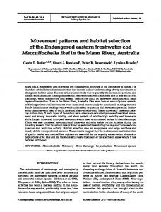
2.3. Methods 2.3.1. Study Area. Research was conducted across three study areas located principally across Kajiado and Narok Counties in southwest Kenya (Fig. 2.1). These areas, referred in the text as the Amboseli Basin (2◦ 30’S, 37◦ 15’E), Athi-Kaputiei Plains (1◦ 30’S, 36◦ 55’E), and Mara (1◦ 15’S, 35◦ 20’E), represent portions of the wildlife dispersal areas in and around Amboseli National Park, Nairobi National Park, and the Maasai Mara National Reserve, respectively. I use these names as a means of convenience to reference the geographic regions where wildebeest were initially collared, even though some animals monitored moved extensively beyond the extent of these areas throughout the course of our study period. Thus, our description of each area includes additional habitats and portions of ecosystems that are not normally considered part of these singular areas, especially as it relates to the Mara. A strong southeast to northwest rainfall gradient occurs across the study areas, which relates to the relative productivity of each system. The Amboseli Basin is the least productive of the three study areas, with rainfall averaging 370 mm yr−1 (range [1998-2013]: 300-525 mm yr−1 , (Xie and Arkin, 1997)). Rainfall across the Athi-Kaputiei Plains averages 475 mm yr−1 annually (range [1998-2013]: 415-570 mm yr−1 , (Xie and Arkin, 1997)), representing 10

moderate levels of productivity. The Mara is the most productive of our three study areas, averaging 665 mm yr−1 (range [1998-2013]: 350-1425 mm yr−1 , (Xie and Arkin, 1997)). April is generally the wettest month of the year, with the majority of rainfall falling during two rainy seasons (short rains: November-December; long rains: April-June). A more detailed description of each study area is provided below. 2.3.1.1. Amboseli Basin. The Amboseli Basin (6,600 km2 ) is a semi-arid tropical environment located in the rain shadow of Mount Kilimanjaro. Our description of this area extends from Longido in Tanzania to the Chyulu Hills in Kenya, the extent of observed wildebeest movements across this ecosystem (Fig. 2.1). Amboseli National Park (400 km2 ) lies at the center of this study area, providing formal protection to a small portion (6%) of the range in which wildlife disperse. The area is covered primarily by open grassland, with woodlands and swamps fed from mountain run-off prevalent in the southern part of the ecosystem (Western, 1973). During the dry season, most species of wildlife and livestock are limited to the immediate basin vicinity where permanent water exists. In wet season periods, species disperse and are more widespread across the ecosystem. Over the past few decades, widespread changes have occurred across the region, with average annual temperature increasing in all months of the year, but particularly in months with higher maximum temperatures (e.g., January - March) (Altmann et al., 2002). Rainfall has remained consistently low throughout the long dry season (June - October), with seasonal timing becoming more variable (Altmann et al., 2002). Woodlands, formerly dominated by Acacia (xanthophloea and tortilis), are increasingly being replaced by shrubs dominated by salt tolerant halophytes (Altmann et al., 2002).

11

Traditional pastoralism is the dominant land-use across the region. Livestock density and grazing pressure is high, a factor leading to habitat degradation and changes to the woodland-grassland mosaic (Altmann et al., 2002). Human population density has remained

Figure 2.1. Wildebeest movements (colored lines) tracked (2010-2013) across three study areas in Kenya (A = Mara, B = Athi-Kaputiei Plains, C = Amboseli Basin). Protected areas (1 = Maasai Mara National Reserve, 2 = Serengeti National Park, 3 = Nairobi National Park, 4 Amboseli National Park) partially obscured. 12

low across the ecosystem, averaging 14 people km−2 (LandScan, 2008). Climate remains the main determinant controlling wildebeest populations, with the recent 2009 drought leading to 97% mortality (6,800 of 7,000 individuals) (Western, 2010). 2.3.1.2. Athi-Kaputiei Plains. The Athi-Kaputiei Plains (3,425 km2 ) were once reported to support some of the highest densities of wildlife in all of East Africa (Simon, 1962). In the last half-century, however, human settlement has expanded rapidly across the region, reducing and fragmenting the remaining habitat and resulting in precipitous wildlife population declines (Ogutu et al., 2013). Reid et al. (2008) estimate a 72% population decline in wildebeest from 1977-2004, with most recent estimates (Ogutu et al., 2013) indicating that population declines could be as high as 93% (a decline from 25,765 to 1,700 individuals). The area is sometimes referred to as the three ‘triangles’ (Fig. 2.1). The first triangle, bordered to the north by Nairobi National Park (112 km2 ) and located just 10 km from Kenya’s capital city, Nairobi, is the northernmost section of this landscape. Human population density is greatest across across this area, averaging 50 people km−2 (LandScan, 2008). Open habitat still exists in the eastern and southern part of the ecosystem (described as the 2nd and 3rd triangle, respectively), although these areas too are threatened with development (e.g., construction of the Konza Technology City, located in the 2nd triangle, has already begun). Livestock raising continues to be the dominant livelihood. Readers are directed to Reid et al. (2008) for images depicting the extent of fencing that have occurred across this region, resulting in a 19% reduction in area accessible to wildlife. A major highway, connecting Kitengela with Kajiado and demarcating the boundary between the 1st and 2nd triangle, also separates the traditional dry and wet season range of the species, bisecting a major migratory route.

13

Soils are rich and comprised predominantly of clay (Ogutu et al., 2013; Reid et al., 2008). Grasses include Pennisetum mezianum, Bothriochloa insculpta, Themeda triandra, and Digitaria macroblephora (Foster and Coe, 1968). Wooded areas consist of Acacia drepanaolobium with A. xanthophloea, Croton macrostachys, and Olea africana located in more densely forested areas (Reid et al., 2008). 2.3.1.3. Mara. The Mara, as referred to here, is the largest of the three study areas (19,200 km2 ). Extending across portions of the Serengeti-Mara ecosystem in Kenya and Tanzania, this area includes the Loita Plains, Mara Plains, Maasai Mara National Reserve (MMNR), Loliondo Game Controlled Area, Ngorongoro Conservation Area, and Serengeti National Park (Fig. 2.1). A series of conservancies also lie adjacent to and north of the MMNR (1,505 km2 ), extending across 960 km2 of the Mara Plains. Maasai pastoralists area restricted from the MMNR, but granted limited access to the conservancies during the dry season. This area is bounded by the Siria Escarpment to the west, the forested Mau Uplands to the north, and the Loita Hills to the east. Large-scale mechanized agriculture has occurred across the northern and western boundary of this ecosystem (Homewood et al., 2001; Serneels and Lambin, 2001), resulting in sharp declines in wildebeest (Serneels et al., 2001). From 1977 to 1997, resident wildebeest declined from 119,000 to 22,000 individuals, an 81% population decline (Ottichilo et al., 2001). Human population density across this study area averages 15 people km−2 , with higher densities (27 people km−2 ) occurring in the Kenyan portion of the area where research was primarily focused (LandScan, 2008).

2.3.2. Wildebeest Movement Data. Thirty-six adult wildebeest were opportunistically captured across the three study areas (National Council for Science and Technology 14

R research permit no. NCST/RR1/12/1/MAS/39/4), fitting animals with Lotek WildCell

GPS collars. Collaring activities occurred in May 2010 across the Mara (n=15) and in October 2010 across the Athi-Kaputiei Plains (n=12) and the Amboseli Basin (n=9). No animals were collared within national park/reserve boundaries. All collared individuals were selected from distinct groups. The mean pairwise distance between initial locations was < 13 km in the Amboseli Basin, < 27 km in the Athi-Kaputiei Plains, and < 22 km in the Mara. Animals were darted intramuscularly with etorphine (M99) and xylazine and processed, on average, in < 20 minutes. The anaesthesia was reversed using diprenorphine (M5050) and atipamezole after fitting the GPS collar. Wildebeest were visually monitored for up to 1 hour, resuming normal activity shortly after drug reversal. All aspects of animal handling were conducted under the direction of a Kenya Wildlife Service field veterinarian and approved by the International Animal Care and Use Committee (IACUC) at Colorado State University, Fort Collins, Colorado, USA (Approval No. 09-214A-02). Devices were programmed to collect sixteen positions per day (every hour during the day (6 AM - 6 PM) and every three hours at night (6 PM - 6 AM)) over a two-year study period. I filtered the dataset, removing suspected erroneous data points using the positional accuracy information output with each data point. Three-dimensional positions with a positional dilution of precision (PDOP) > 10.0 and two-dimensional positions with a PDOP > 5.0 were removed (Appendix A.1). One-dimensional positions were removed. Data were projected to Albers Equal Area projection, WGS84. The gender, approximate age (estimated from tooth wear), and start/end dates of the collaring period are summarized in Table 2.1. Fix success and the fate of each animal are summarized in Appendix A.2.

15

Table 2.1. Summary of GPS collared white-bearded wildebeest (Connochaetes taurinus) monitored across three study areas in Kenya. Mean/Maximum Displacement is the average/maximum net squared displacement from initial collaring locations.

ID

Sex Age

Total Mean Maximum Movement Displacement Displacement (km) (km) (km)

Start Date

End Date

11-Oct-2010 12-Oct-2010 10-Oct-2010 10-Oct-2010 11-Oct-2010 11-Oct-2010 10-Oct-2010 12-Oct-2010 11-Oct-2010

8-Jul-2011 8-Oct-2012 15-Jan-2013 7-Apr-2012 29-Oct-2012 16-Feb-2011 12-Dec-2010 1-Jun-2011 10-Jun-2012

2023.3 6197.8 5604.4 3023.7 5895.9 1146.1 872.1 2502.5 5547.8

11.7 15.5 10.0 18.3 20.8 27.5 17.3 15.0 17.2

44.4 61.8 25.8 41.7 52.1 56.8 34.4 31.4 54.1

Athi-Kaputiei Plains 2840 M 6 15-Oct-2010 2842 M 5 15-Oct-2010 30068 F 9 16-Oct-2010 30070 F 8 20-Oct-2010 30071 F 9 19-Oct-2010 30072 F 9 18-Oct-2010 30074 F 9 16-Oct-2010 30077 F 10 19-Oct-2010 30079 F 9 21-Oct-2010 30082 M 10 17-Oct-2010 30084 M 8 19-Oct-2010 30086 M 10 16-Oct-2010

13-Sep-2011 17-Mar-2012 25-Dec-2010 14-Jun-2011 11-Jan-2013 19-Oct-2012 15-Jan-2013 20-Nov-2012 17-Oct-2012 15-Jan-2013 8-Dec-2011 5-Feb-2012

1628.2 2467.4 324.0 1037.8 2759.1 2386.7 2891.9 3182.4 3187.8 2556.0 1794.1 1634.4

12.2 3.4 1.2 11.1 2.7 1.0 5.1 14.0 6.2 1.2 2.1 1.2

30.0 13.2 5.5 34.6 23.5 7.2 25.4 34.1 38.2 22.9 6.7 11.4

Mara 2829 2830 2831 2832 2833 2834 2835 2836 2838 2839 2841

21-Jun-2012 18-Aug-2010 13-Jun-2012 15-Jan-2013 18-Mar-2011 18-Dec-2011 24-Nov-2010 10-Dec-2012 12-Mar-2011 27-Sep-2011 14-Jun-2010

4117.9 333.2 3042.1 5354.0 1384.3 4257.5 617.4 4676.1 1747.9 2283.2 87.7

21.2 1.9 18.1 7.6 1.8 45.2 2.7 28.6 36.0 4.6 1.1 Continued on

Amboseli Basin 2837 M 9 30069 F 10 30073 F 7 30075 F 6 30076 F 10 30078 F 10 30081 M 8 30083 M 9 30085 M 8

F F M F F F F M F M M

9 10 5 8 7 7 10 9 12 10 8

28-May-2010 28-May-2010 26-May-2010 27-May-2010 28-May-2010 30-May-2010 26-May-2010 30-May-2010 29-May-2010 26-May-2010 29-May-2010

16

40.5 6.6 26.7 25.7 8.2 205.4 9.4 64.1 76.9 29.7 3.4 next page

Table 2.1 – continued from previous page

ID

Sex Age

2843 2844 2845 2846

F F F M

12 7 8 10

Total Mean Maximum Movement Displacement Displacement (km) (km) (km)

Start Date

End Date

27-May-2010 27-May-2010 29-May-2010 25-May-2010

28-Mar-2011 15-Jan-2013 24-May-2012 11-Aug-2011

1562.6 3915.6 4197.0 2177.7

5.3 1.4 45.1 6.8

21.2 16.5 138.1 25.2

Mean: Std Dev:

2735.5 1673.6

12.3 12.1

37.6 38.6

2.3.2.1. Quantifying Individual Movement. I calculated hourly and daily movement rates, net squared displacement, tortuosity, and circular statistics for all animal movement paths throughout the study period. I defined tortuosity as the daily distance moved by each individual divided by the daily maximum net squared displacement, such that animals moving in a straight line would have a tortuosity = 1. The mean resultant length, ρ, was calculated to estimate the concentration of hourly turning angles, with values close to 1 being highly concentrated around the mean. I tested for significant differences between movement statistics by performing Kruskal-Wallis tests and post hoc tests for multiple comparisons in R [R Development Core Team (2013); library pgirmess, function kruskalmc, Siegel and Castellan (1988)]. To compare annual movements across each study area, I subset the dataset to include only those animals that were monitored over the same temporal period, standardizing the start/end dates to 21-October-2010 - 20-October-2011. This reduced the total number of animals being compared to n = 21 (Appendix A.3). Data gaps (< 5% of each dataset) were filled with linear interpolation, the most conservative method for estimating missing locations (Tremblay et al., 2006). I filtered this dataset to longer temporal periods (i.e., 1-day, 17

2-day, 4-day, 8-day, and 16-day) to investigate the interaction between temporal resolution and annual movement across each population (Mueller et al., 2011). Annual movement and temporal resolution were log transformed and fit in a linear mixed model framework [function lme, R library nlme (Pinheiro et al., 2014)], with individual specified as the random effect. 2.3.2.2. Quantifying Population-level Movement. I calculated two measures, the realized mobility index (RMI) and the movement coordination index (MCI), to investigate population-level movement patterns across each study area. Described by Mueller et al. (2011), the RMI is the proportion of habitat occupied by each individual in relation to the total range of the collared population (i.e., the combined annual range of each individual within the population). I calculated the minimum convex polygon range of each individual and computed the RMI as the area of each individual range divided by the combined area of the entire population. The MCI is based on the X and Y shifts among individuals at each movement step and captures variation in both direction and distance. The MCI (from Mueller et al., 2011) can be written:

PN M CItemporalperiod(16−day) =

¯| i=1 |xi − x + P N |x | i i=1

PN

¯| i=1 |yi − y P N i=1 |yi |

!

where xi and yi represent the observed displacements of the ith individual along orthogonal axes in a movement step. N is the number of individuals. Similar to a cross-correlation analysis, the MCI is less sensitive to outliers and does not over-emphasize large deviations from the mean (Mueller et al., 2011). Identical movements among individuals (in direction and distance) yield MCI = 1, with more independent and random movements yielding MCI values closer to 0. 18

Wildebeest across the Athi-Kaputiei Plains were assumed to represent two distinct populations, based on collaring locations (Fig. 2.1) and observations from field efforts over a 2-year study period, and were analyzed separately. I refer to these populations as the Athi-Kaputiei Plains ‘western’ and ‘eastern’ populations (Appendix A.3), signified by their location relative to the Athi-Namanga road that bisects the two groups (Fig. 2.1). Results of the RMI and MCI analyses are representative of the full 1-year dataset, with the MCI analyzed only on animals filtered to the 16-day temporal period. 2.3.2.3. Quantifying Landscape Dynamics. To describe spatial-temporal changes in resources across each study area, I analyzed MODIS Normalized Difference Vegetation Index (NDVI) data (Carroll et al., 2004). NDVI is known to be a direct measure of an areas vegetation productivity/greenness (Goward and Prince, 1995; Tucker, 1979) and has been shown to be an important predictor of ungulate movement and use (Boone et al., 2006; Hopcraft et al., 2014; Pettorelli et al., 2005; Ryan et al., 2012). NDVI from MODIS are provided as 16-day cloud-free data composites (i.e., 23 images per year) with 250-m spatial resolution. I extracted raster subsets from the minimum convex polygon (MCP) of wildebeest locations across each study area, buffered by 10-km, over a 10-year period (2004-2013). Using the semi-monthly NDVI data, I calculated the temporal variability, spatial variability, and unpredictability of each landscape, as described by Mueller et al. (2011). Temporal variability was calculated by summarizing the mean NDVI across space to provide an estimate of resource phenology within years (i.e., the spatial average of the mean NDVI of all images within a semi-monthly period). To estimate the spatial variability across each landscape, I calculated the temporal average of semi-variograms with lags from 5- to 55-km,

19

providing a measure of how resource availability varied across different spatial scales. Unpredictability characterizes the variation across each landscape from year to year (i.e., the repeatability (or lack thereof) of the landscape) (Mueller and Fagan, 2008). To estimate unpredictability, I calculated the spatial average of the standard deviations of NDVI at each grid cell across all images within a semi-monthly period.

2.4. Results 2.4.1. Summary of Movement. GPS collars functioned for 16 - 964 days (mean = 518 days) and collected 279,718 fixes. Average fix success was 94.4% (range = 79.3 - 100.0%) (Appendix A.2). One wildebeest across the Amboseli Basin moved 6,197.8 km over a 728 day study period, the longest distance traversed by any animal monitored. A second wildebeest, animal 2834, moved south from the Loita Plains to the Ngorongoro Conservation Area in Tanzania (Fig. 2.1), a total net displacement of 205.4 km from its initial collaring location. Across the Athi-Kaputiei Plains, no animal was observed to cross the tarmac road (AthiNamanga road, Fig. 2.1) bisecting the seasonal habitat range of the species. Information on collar function is provided in Appendix A.2, with images depicting the movements of each animal in Appendix A.4. Thirty-four percent (33.7%) of GPS locations (21,075 of 62,392) were located within the national park boundary across the Amboseli Basin. Only 3.8% of locations (3,795 of 101,265) across the Athi-Kaputiei Plains and 8.0% of locations (9,228 of 116,061) across the Mara were observed within national park/national reserve boundaries (Fig. 2.1). Wildebeest across the Mara, however, used the conservancies located to the north of the Maasai Mara National Reserve heavily, increasing the percentage of locations within protected area boundaries to 73.4% (85,194 of 116,061) when included. 20

Figure 2.2. Summary of annual movements (A), realized mobility (B), average displacement (C), and movement coordination (D) across three populations of resident wildebeest. Data were subset to the same temporal period (21-Oct-2010 - 20-Oct-2011). Results of the movement coordination index (MCI) are measured in 16-day intervals. Identical movements across individuals have a MCI value of 1. Random movements have a MCI closer to 0 (Mueller et al., 2011). The Athi-Kaputiei Plains population has been split into a western (Athi (west)) and eastern (Athi (east)) population for the RMI and MCI. See Methods for details.

Hourly movements peaked crepuscularly and were greatest across the Amboseli Basin (mean = 407.6 m hr−1 , SD = 204.4). Across the Mara and the Athi-Kaputiei Plains, hourly movements averaged 258.0 m hr−1 (126.7) and 184.8 m hr−1 (93.5), respectively. Table summaries of hourly movements are provided in Appendix A.5 and A.6. Circular statistics highlight that wildebeest movements were most directed (ρ = 0.44) across the Amboseli Basin between 7:00 - 8:00 AM (Appendix A.5). Similarly, although to a lesser degree, wildebeest 21

movements across the Mara and the Athi-Kaputiei Plains were most directed during this same time period (ρ = 0.37 and ρ = 0.27, respectively; Appendix A.5). Wildebeest across the Amboseli Basin moved more per day (8.2 km day−1 , SD = 2.3) than wildebeest across the Athi-Kaputiei Plains (3.6 km day−1 , SD = 0.6, P < 0.001) or the Mara (4.6 km day−1 , SD = 0.9, P < 0.001) (Appendix A.7). No significant difference in mean daily movement was observed between Athi-Kaputiei Plains wildebeest and the Mara population (P > 0.05). These results were consistent with results of the mean daily displacement. Tortuosity was also consistent across study areas, with no statistical difference between populations observed (P > 0.05) (Appendix A.7).

2.4.2. Population-level Movement. Comparing animals with location data subset to the same temporal period, wildebeest across the Amboseli Basin moved the furthest annually (mean = 2,827.2 km yr−1 , SD = 602.8, n = 5), significantly different (P < 0.01) than wildebeest across the Athi-Kaputiei Plains (1,385.2 km yr−1 , SD = 265.6, n = 9) (Fig. 2.2). Mara wildebeest (2,127.9 km yr−1 , SD = 572.0, n = 7) were not significantly different from either population (P > 0.05). Wildebeest across the Mara ranged across the largest area (Fig. 2.1) and were also observed to have the greatest range in displacement among individuals (mean displacement = 22.8 km, range = 0.7 - 66.7 km). Mean displacement was 3.1 km (range = 0.6 - 7.1 km) across the Athi-Kaputiei Plains and 17.3 km (range = 6.7 22.6 km) across the Amboseli Basin (Appendix A.3). Mean displacement, however, was not significantly different between populations (P > 0.05) (Fig. 2.2). The Realized Mobility Index (RMI) indicated a high degree of overlap among the movement ranges of individual wildebeest across the Athi-Kaputiei Plains (western population) (mean = 0.50 range = 0.20 - 0.71) and the Amboseli Basin (mean = 0.44, range = 0.08 22

Figure 2.3. Annual movement in relation to temporal resolution of wildebeest across three study areas in Kenya. Regression lines are species estimates from a linear mixed-effects model.

0.77). Less overlap was observed across the Athi-Kaputiei Plains (eastern population) (mean = 0.26, range = 0.07 - 0.82) and the Mara (mean = 0.24, range = 0.00 - 0.81), with most individuals covering only a small portion of each population range (Fig. 2.2). The movements 23

of individuals within each population were uncoordinated, with no significant difference observed in the movement coordination (MCI) across populations (P > 0.05). The MCI was low across all populations (Amboseli Basin = 0.06, Athi-Kaputiei Plains (western) = 0.06, Athi-Kaputiei Plains (eastern) = -0.06, Mara = -0.06), with a maximum MCI of 0.72 observed across the Amboseli Basin during a single 16-day time period (Fig. 2.2). Analyses of annual movement were nearly identical across the Mara and Amboseli Basin, with no significant difference (P > 0.5) observed in the slope or intercept across different temporal resolutions (1-day, 2-day, 4-day, 8-day, 16-day) (Fig. 2.3). Significant differences (P < 0.01), however, were observed in both the slope and the intercept of regression lines when comparing Athi-Kaputiei Plains wildebeest with animals from the other two study areas. This is an indication that the movements of wildebeest across the Athi-Kaputiei Plains are more tortuous than the movements of wildebeest across the Amboseli Basin or Mara (Fig. 2.3).

2.4.3. Landscape Dynamics. Pronounced spatio-temporal variability in vegetation productivity was observed across the Amboseli Basin and the Athi-Kaputiei Plains (Fig. 2.4). Less variability was observed across the Mara, although increased variability was observed during the long dry season (June - November). Variability generally increased at broader spatial scales, and was highest across the Amboseli Basin from November to April and the Athi-Kaputiei Plains during the long dry season. Similar seasonality patterns were observed across each study area, with the Athi-Kaputiei Plains exhibiting the greatest degree of landscape seasonality and the Amboseli Basin the least (Fig. 2.5A). Across the Mara, landscape unpredictability peaked from December - June (day 321 - 161). Landscape unpredictability across the Athi-Kaputiei Plains was similar 24

Figure 2.4. Semi-variance of productivity based on 10-years (2004-2013) of MODIS normalized difference vegetation index (NDVI) data across the Mara, Athi-Kaputiei Plains, and the Amboseli Basin. Study areas defined by the minimum convex polygon (MCP) from wildebeest relocation data.

25

Figure 2.5. Comparison of landscape phenology across three landscapes in southern Kenya with regard to vegetation biomass (A) and landscape unpredictability (B). Analyses based on 10-years (2004-2013) of MODIS NDVI data. to the Mara, with the short rains (February - April; day 49 - 81) being marginally more predictable across this region. Landscape unpredictability was lowest across the Amboseli Basin, with the long dry season (June November; day 177 - 305) being the most predictable feature across each study area (Fig. 2.5B).

2.5. Discussion Following methods described by Mueller et al. (2011), I provide detailed information on the movements of three populations of wildebeest that have experienced recent and widespread population declines. This analysis compliments previous work completed on these populations, including analyses of space use (Stabach et al. in prep) and the effects of habitat disturbance on fecal glucocorticoid metabolites (i.e., stress hormones) (Stabach et al., 2015). In addition, by analyzing movement across three study areas with differing levels of natural 26

and anthropogenic disturbance, I provide insight into the likely effects of future conditions on individual animal movement. Movement is intimately linked with an animal’s fitness, facilitating an animal’s ability to access better quality resources, encounter potential mates, and move away from an area when conditions deteriorate. Wildebeest across the Amboseli Basin moved more than wildebeest across the Mara and the Athi-Kaputiei Plains in almost every category measured. This was an expected result considering the limits on productivity and the low-levels of anthropogenic disturbance across this arid landscape. Wildebeest across the Athi-Kaputiei Plains, however, moved less than expected based on landscape productivity alone. I expected annual and daily movement to be less across the Athi-Kaputiei Plains than movement across the Amboseli Basin because better quality resources should reduce an animal’s requirement to move. But, Athi-Kaputiei Plains wildebeest also moved less than wildebeest across the Mara, the study area with the greatest availability of resources. While lowered intraspecific competition resulting from observed wildebeest declines could contribute to a decreased need to move and locate resources, stocking rates of domestic livestock are high, with cattle competing with wildebeest across the area for resources. Thus, it is more likely that the observed decrease in movement of wildebeest across this study area is the result of increased levels of anthropogenic disturbance (e.g., roads, fences) and not due to a lack of competition. This is clearly evident related to the decline in annual movement when observed across longer temporal periods, indicating more tortuous (i.e., less directed) movement paths in wildebeest across this region (Fig. 2.3).

27

I also incorporated two additional metrics (the Movement Coordination Index (MCI) and the Realized Mobility Index (RMI) (Mueller et al., 2011)) to describe animal movement. Movement coordination (MCI) was similar across each study area, although highest across the Amboseli Basin, with wildebeest demonstrating near random movements. These results indicate that collared animals were distributed in separate groups and that animals reacted independently to fine-scale resource dynamics. Realized Mobility (RMI) was highest across the Athi-Kaputiei Plains (western population) and the Amboseli Basin, indicating a high degree of range overlap between individuals across these regions. Lowest RMI values were observed across the Mara. The RMI of the eastern population of Athi-Kaputiei Plains wildebeest was also significantly lower than that of the western population, indicative of additional space available to wildebeest across the eastern portion of this study area. Fencing and anthropogenic disturbance are considerably lower across this portion of the Athi-Kaputiei Plains, potentially providing increased habitat suitability for remaining wildebeest. Analyses of landscape dynamics indicate that the Amboseli Basin has the greatest degree of variability across different spatial and temporal scales. This is due to differences between (1) the dense green vegetation located in the swamps within the national park boundary and the dry, low quality vegetation that exists across the remainder of the ecosystem and (2) productivity in dry season and wet season periods. Seasonality was also most predictable across this study area, indicating that although variability exists related to the timing of the start and end points (Altmann et al., 2002), dry seasons in the Amboseli Basin are far less variable when compared to either the Mara or Athi-Kaputiei Plains; a factor known to lead to migratory movement patterns (Mueller and Fagan, 2008; Mueller et al., 2011). Wildebeest across the Amboseli Basin are largely restricted to obtaining water from the swamps within

28

the national park during the dry season, dispersing away from the national park daily and during wet season periods to exploit resources with lower levels of competition (Appendix A.4). The Mara is the most productive of our study areas, with less variability across different temporal and spatial scales than the Amboseli Basin or Athi-Kaputiei Plains. The observed variability is less predictable between years, however. Consequently, I observed a mixture of movement strategies across this study area, which include nomadism, range residency, and migration (Appendix A.4). The lack of exclusivity is a common problem when attempting to characterize population-level movements from analyses of individual animals (Mueller et al., 2011), with an animals sex, reproductive status, and social status all having potentially confounding effects on movement. Across the Athi-Kaputiei Plains, wildebeest are almost exclusively range residents (Appendix A.4). It is unclear, however, the degree to which the movement strategies of animals across this landscape are dictated by the observed levels of anthropogenic disturbance. Collared wildebeest were located primarily outside of protected area boundaries throughout our study period. This is an interesting result considering the low levels of anthropogenic disturbance found within the boundaries of these areas, especially across the Athi-Kaputiei Plains where high levels of anthropogenic disturbance lie directly adjacent to the national park boundary. The observed effect could be reflective of differences in vegetative quality, predation pressure, or alternatively, a result of capture-induced bias, since animals were not fit with collars within national park/reserve boundaries. Additional research is assuredly necessary to confirm these results. Across the Athi-Kaputiei Plains, results are at least partially biased by the Athi-Namanga road, as wildebeest did not move between the 1st and 2nd triangles during the study period. Wildebeest collared in the 2nd triangle were therefore

29

unable to disperse to the national park. These data also provide quantitative support that this historic local migration may have collapsed, with no collared wildebeest crossing the road over the length of the study period. My results also have important conservation implications across the region that can be applied to other systems, especially dryland systems where the ability of species to move between seasonal habitat ranges is essential for survival. Animals collared across the AthiKaputiei Plains were observed with a single movement strategy (i.e., range residency), a stark contrast to the Mara. In years of high levels of productivity, the restrictions on movement likely have minimal effects on animals across this landscape, with the available habitat seemingly providing the necessary requirements for extant animals to meet energy demands. In excessively dry years, animals simply have no place to disperse. Unlike the Amboseli Basin, where wildebeest are in the process of recovering from the multi-year drought that caused extreme mortality in 2009, habitat isolation resulting from anthropogenic disturbance across the Athi-Kaputiei Plains could result in a population that is unable to recover. Pastoralists across the region recognize this threat, voicing concern about how and where they will find suitable habitat for their livestock in times of drought. Road construction is also a consistent threat across this region, and which has been debated for years related to the potential effects of a road constructed to connect rural communities across the Serengeti ecosystem (Dobson et al., 2010). While I did not set out specifically to address this issue, my results clearly illustrate the effect that a developed road (and the increased human land-uses that often develop alongside them) can have on wildebeest movement and dispersal. While the Athi-Namanga road represents a road with

30

greater road traffic volume and road-side development than is envisioned across the Serengeti ecosystem, the threat to migrating animals is too great to risk. By linking the movements of wildebeest across three study areas in Kenya with dynamics of landscape productivity, I provide a greater understanding of how broad-scale landscape changes effect individual movement patterns. The most predictable and dynamically changing landscape, the Amboseli Basin, led primarily to local-scale migratory-type movement. The Athi-Kaputiei Plains was both more predictable and more variable than the Mara, with wildebeest across this study area ranging across the smallest areas and moving the least per day among the study areas monitored. Anthropogenic habitat disturbance likely acts as a key contributor limiting movement across this study area, with wildebeest moving far less than expected based on landscape productivity alone. Mara wildebeest had the greatest range in movements, with some animals dispersing long distances while others remained locally resident throughout the entire study period. Taken together, these results provide an increased understanding into the likely effects of future conditions on wildebeest movements, an important determinant on the long-term sustainability of these threatened populations.

31

CHAPTER 3

Mixed movement strategies in resident white-bearded wildebeest 3.1. Summary 1

In order to optimize access to resources and minimize risk of predation or conflict,

animals structure their spatial behaviour by switching between different movement states, classically defined as encampment, exploration, or nomadism. In some dynamic environments, the combination of these movement states results in migration, a tactic employed to access resources that vary spatially and/or temporally in a predictable manner. While most populations can be characterized discretely as adhering to a specific strategy (i.e. migratory or non-migratory), systems with mixed strategies are increasingly recognized. The distinction between individual strategies in such systems and related drivers remain poorly defined. I investigated the movement strategies of Mara wildebeest, a sub-population of the greater Serengeti wildebeest population, alleged to be non-migratory and restricted to the northern range of the ecosystem. Using analyses of movement metrics (displacement distance, linearity and range size) and conducted in a Bayesian framework, I distinguish two categories of movement among individuals within this local population, with a ‘migratory’ class of individuals that displaced nearly 5 times as far from initial collaring locations and moved 1.8 times the distance per day as ‘residents’. A third movement state was identified when incorporating GPS data from the Serengeti migratory herd, with Serengeti migrants moving further per day than either of the Mara wildebeest categories. Contrary to simple expectations, this 1A

version of this chapter has been submitted for review at Animal Conservation with co-authors George Wittemyer, J. Grant C. Hopcraft, Randall B. Boone. 32

work demonstrates that the resident Mara wildebeest, a sub-population that has experienced widespread decline, employs a mixture of movement strategies that likely relate to its ability to cope with changing resource dynamics and rapid landuse changes occurring across this ecosystem. Further, this study provides a framework for identifying where individuals fall along the migratory-resident movement continuum based on movement metrics.

3.2. Introduction Movement is a fundamental aspect of animal ecology, enhancing an individual’s ability to obtain resources, encounter potential mates, avoid predation, or disperse from an area when conditions deteriorate. Many studies have focused on quantifying different movement states (Fryxell et al., 2004, 2008; Dalziel et al., 2008; Bunnefeld et al., 2011; Singh et al., 2012) classifying movement as encamped/residential, exploratory/migratory, or nomadic. In most systems, however, animals exhibit a mixture of movement strategies across time, making exclusive assignment into one particular category difficult (Mueller and Fagan, 2008; MilnerGulland et al., 2011; Singh et al., 2012). As such, movement strategies can be thought of as a continuum across these common classifications. Identifying where a species, population, or individual falls along this continuum is important both for understanding conservation threats and management needs. There is increased concern about the sustainability of long-distance migrations (Berger and Barbieri, 2004; Bolger et al., 2008; Wilcove and Wikelski, 2008; Harris et al., 2009; Dobson et al., 2010), especially across terrestrial environments where habitats are becoming increasingly fragmented or lost altogether due to competing human demands. For large mammals, the connectivity of landscape patches is essential to allow animals to move from areas of poor habitat quality when conditions deteriorate (Owen-Smith, 2004). Across the 33

Mara Plains, a dryland system in southern Kenya that is the northernmost section of the Mara-Serengeti ecosystem, expansion of mechanized agriculture and increased large-scale ranching have decreased the total area available to grazers and fragmented portions of the remaining habitat (Serneels et al., 2001; Homewood et al., 2001), leading to an approximate 81% decline in this population of white-bearded wildebeest (Connochaetes taurinus) (119,000 to 22,000 animals) over the past 30 years (Ottichilo et al., 2001; Serneels and Lambin, 2001; Homewood et al., 2001; Ogutu et al., 2011). Concern exists, not only for this declining resident wildebeest population, but also for the ∼1.3 million Serengeti migratory wildebeest (Thirgood et al., 2004) which rely on this region for annual dry season grazing (NortonGriffiths, 1995). The movement of the ‘Mara resident’ sub-population is largely unknown, despite the threat it faces from landuse changes and fragmentation. To better characterize its spatial needs, twelve Mara resident wildebeest were tracked from May 2010 to January 2013 (Boone et al., 2009) using GPS collars from which I classified their movement strategies along a resident to migratory continuum using a statistically robust approach. I also compared the Mara residents with GPS movement data on five wildebeest from the larger Serengeti migratory sub-population (Thirgood et al., 2004; Hopcraft et al., 2014). The degree of mixing between these two sub-populations is unknown. I discuss the similarities and differences in movement metrics and highlight a simple method that can be used to differentiate migratory from non-migratory individuals within the same population.

3.3. Methods 3.3.1. Study Area. The Maasai Mara National Reserve (MMNR) is the northernmost section of the Serengeti-Mara ecosystem located in southwest Kenya (bounding coordinates: 34

34.7◦ W, 35.4◦ E, -1.2◦ N, -1.8◦ S) (Fig. 3.1) and characterized by open savanna. The MMNR covers an area of 1,506 km2 , with conservancies adjacent to the MMNR covering an additional 960 km2 of the Mara Plains. The Loita Plains are located to the north of the conservancies and are recognized as the prime calving grounds of the resident sub-population. Widespread wheat farming has expanded across this region over the past few decades (Serneels et al., 2001), resulting in precipitous wildebeest declines (Serneels and Lambin, 2001). Traditional agro-pastoralism is practiced by Maasai across this region. Maasai are restricted from the MMNR but granted limited access to the conservancies during the dry season. Seasonality is markedly bimodal with average precipitation ranging from 775 - 1,350 mm yr−1 (Xie and Arkin, 1997). January and April are generally the wettest months.

3.3.2. Wildebeest Position Data. In May 2010, twelve wildebeest (eight female and R four male) were fit with Lotek WildCell Global Positioning System (GPS) collars (Table

3.1) across the Mara and Loita Plains. During this time period, resident wildebeest and migratory wildebeest are located in different geographic areas (i.e., the populations are separate). Thus, it was assumed that collars were deployed only on resident wildebeest, referred to as Mara wildebeest. Animals were opportunistically selected from distinct herds, separated on average by 21.8 km (mean pairwise distance). Approximate age (estimated from teeth wear) at the time animals were collared ranged from 5 to 12 years old. Herd size ranged from 10 to 64 animals, inclusive of adults, juveniles, and calves (Table 3.1). All aspects of animal handling were conducted under the care of a Kenya Wildlife Service veterinarian using nationally approved methods. Handling was approved by the International Animal Care and Use Committee (IACUC) at Colorado State University, Fort Collins, Colorado, USA (Approval No. 09-214A-02). 35

Figure 3.1. Movements (1-year) of GPS collared wildebeest across the Serengeti-Mara ecosystem. Mara residents (n = 9) (dashed lines) and Mara migrants (n = 3) (solid lines) highlighted. Protected areas, including Mara conservancies, displayed. Note that residents are almost exclusively located to the north of the Maasai Mara National Reserve boundary.

GPS collars were programmed to acquire sixteen GPS positions per day, every hour during the day (6 AM to 6 PM) and every three hours nocturnally (6 PM to 6 AM). Erroneous data points were removed using accuracy estimates output with the positions. Only 2D positions with a Dilution of Precision (DOP) < 5.0 and 3D positions with a DOP < 10.0 were included in analyses. In total, 114 798 GPS positions were collected. Data were projected to Albers Equal Area projection, WGS84 datum. 36

Table 3.1. Summary of GPS collared white-bearded wildebeest (Connochaetes taurinus). Age estimated on the collaring date. Herds include adults, juveniles, and calves. Age and approximate herd size not collected (–) for every animal. Dataset was filtered to a 1-day time interval, noon fixes (± 2 h). Unprotected is the percentage of fixes collected to the north of the boundary of the Maasai Mara National Reserve and across the Mara/Loita Plains. Pct is the total number of fixes received (Fixes)/total fixes expected (Period). Serengeti wildebeest from Thirgood et al. (2004) and Hopcraft et al. (2014). ID

Sex Age Herd Unprotected

Mara wildebeest 2829 F 9 12 2831 M 5 64 2832 F 8 13 2833 F 7 51 2834 F 7 – 2836 M 9 11 2838 F 12 22 2839 M 10 39 2843 F 12 12 2844 F 7 25 2845 F 8 18 2846 M 10 16 Serengeti wildebeest W04 F – – W07 F – – W08 F – – W09 F 6 5000 W10 F 6 5000

Start Date

End Date

Fixes Period

Pct

90.9 100.0 100.0 100.0 71.0 94.4 73.2 94.1 95.1 100.0 39.5 99.7

30-May-2010 30-May-2010 30-May-2010 30-May-2010 30-May-2010 30-May-2010 30-May-2010 30-May-2010 30-May-2010 30-May-2010 30-May-2010 30-May-2010

29-May-2011 29-May-2011 29-May-2011 18-Mar-2011 29-May-2011 29-May-2011 12-Mar-2011 29-May-2011 28-Mar-2011 29-May-2011 29-May-2011 29-May-2011

352 353 356 282 356 357 275 354 289 358 355 355

365 365 365 293 365 365 287 365 303 365 365 365

96.4 96.7 97.5 96.2 97.5 97.8 95.8 97.0 95.4 98.1 97.3 97.3

0.0 0.0 3.5 0.0 0.0

1-May-1999 6-Jun-2000 2-Jun-2000 21-Jun-2003 20-Jun-2003

2-Nov-1999 8-Mar-2001 14-Dec-2000 13-Jan-2004 14-Jan-2004

185 231 195 207 209

186 276 196 207 209

99.5 83.7 99.5 100.0 100.0

I standardized the start/end dates that each animal was tracked to a 1-year study period (30-May-2010 29-May-2011) and filtered to a 1-day time interval. Remaining data gaps (< 5% of each dataset) were filled using linear interpolation, conservatively estimating missing locations as the linear midpoint between two observed locations (Tremblay et al., 2006). The resulting dataset represents a complete daily trajectory for each animal (Table 3.1). Additional versions of the data, filtered by longer temporal periods (i.e., 2-day, 4-day, 8-day, 37

and 16-day), were also created. Results when analyzing these datasets representing coarser sampling, however, did not change reported conclusions (provided in Appendix B.1). 3.3.3. Analysis of Movement Patters. I assessed the movements of Mara wildebeest by calculating linear and home range movement metrics. Linear movement metrics consisted of the maximum linear path distance moved by each animal over the study period, the average and maximum daily movement rate, and the average and maximum net squared displacement (as described in Bunnefeld et al. (2011) and Singh et al. (2012)). Home range metrics included the calculation of 100% Minimum Convex Polygons (MCP) (Mohr, 1947), Localized Convex Hull (LoCoH) home ranges parameterized from a fixed number of √ k nearest neighbors (2 k/3)(Getz and Wilmers, 2004; Getz et al., 2007), and the 50% and 90% Gaussian fixed kernels using the reference parameterization (i.e., ‘href’). Movements of collared wildebeest are displayed in Figure 3.1, with individual trajectories of each animal displayed in Appendix B.2. Three animals (2833, 2838, and 2843) were not tracked for the entire 1-year study period (Table 3.2). To include these animals in statistical analyses, I proportionally adjusted the home range metrics and the linear path distance of these animals based on animals that completed the full length of study. That is, I calculated the difference between home range and movement metrics for a 300-day study period (nearly equal to the period that each of the three animals completed the study, Table 3.2) with results calculated over the entire 365-day study period. This method, as opposed to adjusting each metric based on the total number of days tracked, more similarly and conservatively updated the metrics of the three animals with those that completed the study.

38

39

671.1 891.0 997.6 869.8 751.9

3.7 3.3 5.1 4.2 3.6

3.6 3.0 2.7 17.3 23.6 33.0 18.5 23.3

36.9 26.8 20.6 156.8 90.8 101.0 84.2 92.6

36.6 34.6 65.2

211.1 136.5 154.0 136.7 143.8

89.2 75.7 138.2

11903.7 14124.9 14376.0 4515.6 6466.4

4217.4 3128.91 7136.0

1281.2 153.1 259.6 52.21 1263.6 380.1 446.91 11.7 283.1

3987.3 7915.6 4203.1 2753.3 3469.6

1499.6 1538.31 3521.3

409.9 13.1 47.1 5.01 650.6 21.6 56.61 0.8 13.8

389.1 22.5 40.3 14.21 337.1 65.1 102.61 2.5 60.6

LoCoH Area (km2 )

20019.4 26867.6 18543.3 9239.6 11466.5

1202.8 2084.2 2232.1 1100.4 1218.7

5017.6 1211.1 4356.81 639.51 11272.2 1501.5

1345.2 75.5 262.7 30.01 1884.4 190.6 316.01 4.3 115.1

90% Area (km2 )

proportionally updated due to < 365 fixes received. Pertains only to Total Movement and all home range metrics. See text for details.

1 Value

Serengeti Migrants W04 F 185 W07 F 231 W08 F 195 W09 F 207 W10 F 209

1314.2 984.71 998.1

36.1 20.5 22.2 7.0 63.9 25.3 20.2 6.1 18.9

Migrants F 365 F 287 F 365

15.5 2.8 6.0 1.7 32.4 3.6 5.2 1.7 2.7

Mara 2834 2838 2845

27.1 13.8 16.3 7.6 25.9 10.4 12.7 4.3 12.8

Mara 2829 2831 2832 2833 2836 2839 2843 2844 2846 2.5 1.3 1.8 1.2 3.3 1.6 1.7 0.7 1.6

Residents F 365 M 365 F 365 F 293 M 365 M 365 F 303 F 365 M 365

ID 920.5 488.6 646.4 391.71 1183.5 576.7 568.71 270.2 569.8

Total Mean Maximum Mean Maximum 100% 50% Kernel Movement Velocity Velocity Displacement Displacement MCP Area Area Sex Fixes (km) (km/day) (km/day) (km) (km) (km2 ) (km2 )

Table 3.2. Summary of white-bearded wildebeest (Connochaetes taurinus) movement patterns. Results include linear and home range movement metrics. Residents and Migrants were separated using a k -means cluster analysis based on these statistics.

Localized changes in range use were assessed by calculating the arithmetic mean of the X and Y coordinates (Wall et al., 2013). Movements in the north-south direction were considered independently from movements in the east-west direction. I also calculated the Movement Coordination Index (MCI). Formulated by Mueller et al. (2011), the MCI is based on the X and Y shifts among individuals at each movement step and captures variation in both direction and distance. Similar to a cross-correlation analyses, the MCI is less sensitive to outliers and does not over-emphasize large deviations from the mean (Mueller et al., 2011). Identical movements among individuals yield MCI = 1, with more independent and random movements yielding MCI values closer to 0. I calculated the MCI for Mara wildebeest, separated into residents and migrants (see below) for the entire study period and pairwise between animals. Because the number of animals differed between residents and migrants, I used a jackknife procedure when calculating the MCI on residents. Samples were analyzed from three individuals at a time, drawn randomly and without replacement. The process was repeated for 100 iterations, calculating the mean MCI at each movement step, before aggregating the statistic to a mean measure for each temporal period. All movement analyses were calculated in the statistical program R (Version 2.13.1, R Development Core Team (2013)), inclusive of the adehabitatHR/LT (Calenge, 2006), proj4 (Urbanek, 2012), and sp (Pebesma and Bivand, 2005; Bivand et al., 2013) packages.

3.3.4. Distinguishing Movement Strategies among Collared Wildebeest. To distinguish between different movement strategies, I separated Mara wildebeest into two categories (‘Mara Plains residents’ and ‘Mara migrants’) using a k -means cluster analysis (Forgy, 1965; MacQueen, 1967; Hartigan and Wong, 1979). All home range and linear 40

movement metrics (Table 3.2) were input into the clustering algorithm, resulting in nine Mara residents (five female and four male) and three Mara migrants (all female).

3.3.5. Comparison to Serengeti Migrants. To assess if Mara residents/migrants moved similarly to the Serengeti sub-population, I incorporated data from two separate GPS studies on the movements of Serengeti migratory wildebeest (Thirgood et al., 2004; Hopcraft et al., 2014). I refer to these animals as ’Serengeti migrants’. Five female Serengeti migrants, collared for a period of 186 to 209 days, were subjected to the same data cleaning steps as outlined above. I allowed for greater flexibility in the start dates among animals, which ranged from 01-May-1999 to 21-June-2003 (Table 3.1). I assessed the similarity in local conditions between collaring periods by comparing rainfall estimates (Xie and Arkin, 1997) across the time periods. I extracted 10-day (i.e., dekadal) estimates of rainfall from a 10 km buffer around the MCP of each animal and compared the means of these years with the mean and standard deviation (SD) of rainfall across our study period. Year 2003 was wetter than 2010, while years 1999 and 2000 received a similar cumulative amount of rainfall as year 2010 (Appendix B.3).

3.3.6. Statistical Analyses. I tested for statistical differences between the movements of collared wildebeest using hierarchical Bayesian fixed-effect one-way ANOVAs. This analysis method allowed us to make inference on the population and provide statements of the probability that the movement metrics for each group (i.e., Mara residents, Mara migrants, and Serengeti migrants) were derived from the same distribution. Following (Kery, 41

2010) and (McCarthy, 2007), our model specification was:

yijk = αj(i) + i i ∼ N ormal(0, σ 2 )

where yijk is the observed movement metric k (listed in 3.3.3 above) of wildebeest i in population j, αj(i) is the expected movement of a wildebeest in population j, and residual i is the random movement deviation of wildebeest i from its population mean αj(i) . Observations that did not meet the assumptions of normality, assessed using a Shapiro-Wilk test (Royston, 1982) with a significance of p < 0.05, were log-transformed. Table 3.3. Summary of movement statistics of GPS collared white-bearded wildebeest (Connochaetes taurinus). Results include linear movements and home-range metrics. Difference is the probability that the movement statistic mean of migrants was greater than that of residents. Mara Residents

Mara Migrants

Statistic

Posterior Median

95% CI

Posterior Median

95% CI

Total Movement (km) Mean Velocity (km/day) Max. Velocity (km/day) Mean Displacement (km) Max. Displacement (km) 100% MCP Area (km2 ) 50% Kernel Area (km2 ) 90% Kernel Area (km2 ) LoCoH Area (km2 )

656.0 1.7 14.6 4.8 19.7 260.2 28.0 153.0 49.2

(391.1, 906.0) (1.2, 2.3) (8.8, 20.3) (2.4, 9.3) (12.0, 32.5) (69.9, 966.7) (7.0, 113.6) (43.7, 535.9) (17.2, 141.0)

1102.6 3.1 28.1 43.5 97.5 5497.8 2011.3 6269.2 1029.0

(597.1, 1537.9) (2.2, 4.0) (18.1, 38.0) (13.6, 138.7) (41.2, 231.0) (470.7, 64934.4) (178.2, 22768.4) (718.6, 55083.9) (165.5, 6399.0)

Difference 0.948 0.995 0.988 0.998 0.998 0.983 0.997 0.997 0.996

Marginal posterior distributions of parameters were estimated using Markov chain Monte Carlo (MCMC) methods. Analyses were implemented in program R (R Development Core Team, 2013) using the rjags package (Plummer et al., 2010), JAGS version 3.2.0. Each of three MCMC chains was run for 100 000 iterations; the first 20 000 iterations were discarded 42

to allow for burn-in. Convergence was assessed by visual inspection of trace plots to ensure a reasonable exploration of the parameter space, and by ensuring that the potential scale reduction factor was < 1.02 for each variable (Gelman and Rubin, 1992). Results were backtransformed, if necessary. At each MCMC step, I calculated the Bayesian equivalent to a p-value by assessing whether the mean of one group was greater than the other. Sample R code, comparing the median daily movement between Mara residents and Mara migrants, is provided in Appendix B.4.

3.4. Results 3.4.1. Movement Patterns. Mara migrants moved at least double the amount of Mara residents in nearly every movement category (Table 3.3). Mara residents displaced a maximum distance of 19.7 km (posterior median) from initial collaring locations (95% credible interval: 12.0 - 32.5) and spent > 90% of the year to the north of the Maasai Mara National Reserve (MMNR) and outside of formally recognized protected areas. In contrast, the maximum distance (posterior median) displaced by Mara migrants was 97.5 km (95% credible interval: 41.2 - 231.0), nearly 5 times the distance displaced by Mara residents. Mara migrants spent < 75% to the north of the MMNR boundary, with one migrant (ID 2845) spending < 40% of the year in this region (Table 3.1). Similar trends were observed for home range metrics (Table 3.3). The probability that the mean movement metric of the Mara migrants was greater than that of Mara residents was 0.95 for all movement and home range metrics. Posterior medians, 95% credible intervals, and probabilities that the Mara migrant mean was greater than the Mara resident mean are provided in Table 3.3. Animal trajectories and associated home ranges are displayed in Appendix B.2. 43

The Movement Coordination Index (MCI) showed differences between movement categories, with Mara migrants being more coordinated (MCI: 0.13, 95% credible interval: 0.11 - 0.15) than Mara residents (MCI: 0.02, 95% credible interval: 0.01 - 0.04). Pairwise, no two animals had a MCI > 0.26. I also observed a strong north-south movement component among Mara migrants (Appendix B.5). The timing of this movement (i.e., December-January) is past the time period in which Serengeti migratory wildebeest would be expected to have already moved from the area (i.e., October-November; see (Inglis, 1976; Thirgood et al., 2004; Boone et al., 2006; Hopcraft et al., 2014)). The north-south movement of Mara migrants, however, was small in comparison with the extensive (∼200 km) dispersal of Serengeti migrants from the area (Fig. 3.2). Resident wildebeest were remarkably stationary in the north-south direction. In the east-west direction, Mara migrants exhibited greater movement than Mara residents (Appendix B.5).

3.4.2. Comparison to Serengeti Migrants. Serengeti migrants moved more than double the daily movement rate (mean velocity) of Mara residents at 4.0 km/day (95% credible interval: 3.3 - 4.7), which exceeded the daily movement rate of Mara migrants (Fig. 3.3). The probability that the movement rate of Serengeti migrants was greater than the movement rates of Mara residents and migrants was 1.00 and 0.94, respectively. Mara migrants, however, had a maximum daily movement rate (posterior median: 28.1 km/day; 95% credible interval: 18.1 - 38.0) that was greater than Serengeti migrants (posterior median: 23.1 km/day; 95% credible interval: 16.1 - 30.2). The probability that the maximum movement rate of Serengeti migrants exceeded that of Mara migrants was 0.19. The pairwise MCI of Serengeti migrants (W07 and W08) monitored in the year 2000 was 0.29. The MCI for the 44

Figure 3.2. Mean position in the Northing direction for Mara residents (dashed line), Mara migrants (black solid line), and Serengeti migrants (gray solid line). Data plotted against month. Horizontal black lines represent dry season periods in 2010, delineated by incorporating MODIS NDVI data (MOD13Q1) into the TIMESAT software package with a Savitsky-Golay function (Jonsson and Eklundh, 2002, 2004; Eklundh and Jonsson, 2011). Note that the Serengeti migrant data is representative of GPS data from years 1999, 2000, and 2003. The graph highlights the northerly movement of Serengeti migrants towards the Mara wildebeest from June to August, where animals resided during the dry season (August - October). The graph also highlights the departure of Serengeti migrants from the area, pre-dating the southerly movement of Mara migrants by approximately 2-months. two animals (W09 and W10) monitored in 2003 was 0.27, indicating that Serengeti migrants were more coordinated than Mara migrants/residents, but still at a low level of coordination. 3.5. Discussion The Mara-Serengeti migration represents the second longest terrestrial mammalian migration remaining in Africa today (the migration of Burchells zebra (Equus quagga) across 45

Figure 3.3. Daily movement rate posterior distributions of Mara residents, Mara migrants, and Serengeti migrants.

parts of Namibia and Botswana is the longest (Naidoo et al., 2014)). Surprisingly little is known about the movements of wildebeest across this ecosystem, and even less about the space use of the resident population, despite wide recognition of its rapid decline. Only three studies to date have monitored the movements of individual animals (Inglis, 1976; Thirgood et al., 2004; Hopcraft et al., 2014) and each of these studies focused on the larger Serengeti sub-population that calves in the southern Serengeti of Tanzania. Our study is the first to track the threatened sub-population of ’resident’ wildebeest that calves in the Mara of Kenya, providing detailed information about the movements of individual wildebeest within this population and a direct comparison with results presented by Thirgood et al. (2004) and Hopcraft et al. (2014). 46

The approach developed and implemented to distinguish movement strategies (relying on k -means clustering) across individuals in the ecosystem identified two movement strategies employed in the Mara sub-population. It is notable that this straightforward approach can be used to determine the number of distinct groups (e.g., Charrad et al., 2014), though I focused simply on distinguishing migratory from non-migratory due to its conservation relevance. Our results highlight that Mara migrants moved at least twice the amount as their resident counterparts in nearly every movement category, were more coordinated in their movements, and dispersed greater distances in the north-south and east-west directions. These traits provide descriptive evidence and an improved understanding of the movement structure distinguishing migratory from non-migratory individuals. Interestingly, the movements of Mara migrants were consistently less than Serengeti migrants in all assessed categories except for the maximum daily movement rate. The timing of the initiation of longitudinal movements also differed between the Mara migrants and the Serengeti migrants. It is possible that these findings are an artefact of the compared sampling periods, since grass quality is the main driver governing individual wildebeest movements and can vary considerably from year to year (Hopcraft et al., 2014). While further analyses comparing individuals over the same time period are necessary, cumulative rainfall (Appendix B.3) was similar between years compared, providing support for our findings. Our results demonstrate at least three different movement strategies exist among individuals using this area. The Mara herd is much smaller (∼20 000 individuals (Ottichilo et al., 2001)) than the Serengeti herd (∼1.3 million individuals (Thirgood et al., 2004)), with wildebeest rarely observed in groups > 150 individuals. Serengeti wildebeest are often observed traveling in herds of 20,000 - 100,000 individuals. The Mara migrants, therefore, likely face greater

47

predation risk when moving through densely wooded areas, which may account for the observed increase in the daily maximum movement rate relative to the Serengeti population. Alternatively, the increased movement rate could be entirely due to increased human densities found to the north of the MMNR. Animal 2834, for instance, moved further per day than any animal monitored (36.9 km/day). This increased rate of movement occurred when the animal moved south from its initial collaring location in the Loita Plains through a relatively narrow, heavily populated area along the Bardamat Hills (Fig. 3.1). This area forms a pinch point to dispersal between the Loita Plains and the MMNR. Our data show that Mara wildebeest use this area heavily and increase their movement rate when doing so. Determining why individuals adhere to certain strategies was beyond the capacity of this study. However, other migratory systems have identified a genetic component to the migratory strategy taken by an individual (Northrup et al., 2014). It’s possible that Mara wildebeest switch between movement strategies in successive years, which may be related to an animal’s reproductive status. All three animals categorized as Mara migrants, for example, were female. Female wildebeest have the potential to be both lactating and pregnant for a 5-month period between June and October (Hopcraft et al., 2013), with lactating females requiring 30% more energy than females in early pregnancy (Murray, 1995). I did not assess the reproductive status of collared animals, but the increased movement observed in these animals could be due to the necessity to meet energy demands or locate areas that provide specific resources. Of the remaining animals categorized as Mara residents, the sex ratio was nearly 50:50, with one female (ID 2844) moving the least (Table 3.2 ) of any of the animals that were collared. Collecting ancillary data on the reproductive status of collared

48

animals may help explain the patterns that I observed and provide valuable information to investigate changes in movement strategies across years. In order to make comparisons between animals, I analyzed movements only during a 1-year study period. While logistically necessary, this simplifies our inference on movement strategies. Analyses of net squared displacement, often used to determine resident, nomadic, or migratory behaviour (Bunnefeld et al., 2011; Singh et al., 2012), may provide different inference depending on the length of time that movements are analyzed. Over the 1-year study period, for example, Animal 2845 displaced 138.1 km from its initial collaring location and moved in a nomadic fashion (Appendix B.6). When extending the monitoring period to 2-years, this same individual is observed to return to within 5.9 m of its initial collaring location. This suggests that residents probably move between different patches in a similar way as Serengeti migrants, but at a much finer scale. This study highlights three distinct movement strategies employed by wildebeest across the Mara-Serengeti ecosystem. Mara wildebeest spent > 75% of time outside of formally protected boundaries regardless of strategy, emphasizing the importance of conservancies and areas of lesser degrees of protection that are adjacent to the Maasai Mara National Reserve and Serengeti National Park. While additional research (i.e., genetic analysis) is needed to determine the degree of mixing between resident and migratory wildebeest populations, this work defines the mechanistic differences in movement patterns between the Mara and Serengeti wildebeest herds, as well as offering a simple framework for partitioning movement strategies along the continuum of resident to migratory categorization. Such inference provides detailed specification about individual movement strategies to aid conservation and management planning across the region.

49

CHAPTER 4

Habitat disturbance effects on the physiological stress response in resident Kenyan white-bearded wildebeest (Connochaetes taurinus) 4.1. Summary 1

Regarded as a keystone species, white-bearded wildebeest (Connochaetes taurinus) are

found across the grassland savannahs of eastern Africa. Over the past 40 years, however, many local populations have become threatened with extinction. This is the first study connecting fecal glucocorticoid metabolites (i.e., stress hormones) in wildebeest with landscape variables of natural and anthropogenic disturbance. Using a validated technique, fecal samples (n = 168) were collected from wildebeest over a 3-month study period and across three different study areas in Kenya with varying degrees of disturbance. The stress of sampled populations was similar between study areas, with a seasonal decline in stress hormones found between dry and wet season data collection periods. I used an information-theoretic approach to rank models of fecal glucocorticoid metabolites. My highest ranking model included an interaction between locally collected plant biomass and disturbance, the number of calves in a group, and ∆NDVI (change in Normalized Difference Vegetation Index). A strong positive effect related to biomass and disturbance suggested that tall/standing biomass and high levels of disturbance contribute to elevated levels of stress in wildebeest. A strong negative effect related to ∆NDVI was also observed, suggestive that new growth lowers average 1A

version of this chapter has been published in Biological Conservation 182:177-186: Stabach JA, Boone RB, Worden JS, and Florant G. (2015). Habitat disturbance effects on the physiological stress response in resident Kenyan white-bearded wildebeest (Connochaetes taurinus). 50

stress levels. This research suggests that increased levels of habitat disturbance may have an adverse effect on wildebeest populations across the region when habitat conditions deteriorate. Wildebeest likely avoid areas of high anthropogenic disturbance which may indirectly lead to lowered fitness.

4.2. Introduction White-bearded wildebeest (Connochaetes taurinus) are dominant herbivores found across the grassland savannahs of eastern and southern Africa. Perhaps best known for their longdistance seasonal migrations, wildebeest are often required to travel great distances to locate areas of suitable forage, especially during the driest parts of the year when resources are limited. The International Union for the Conservation of Nature (IUCN) currently lists the population as stable (IUCN, 2013). However, this designation relates mostly to the approximate 1.3 million wildebeest found across the Serengeti ecosystem (Thirgood et al., 2004). In other parts of the species range and most specifically in Kenya where research is focused, widespread and precipitous declines have been recorded (Estes and East, 2009; Ogutu et al., 2011, 2013; Ottichilo et al., 2001; Reid et al., 2008). Directly related to these population declines is the pervasive expansion of mechanized agriculture and large-scale ranching that have occurred across the region (Serneels and Lambin, 2001). These processes fragment the landscape, forming habitat discontinuities and imposing barriers (e.g., roads, fences) to daily and seasonal movement. Over the past 3 years, the movements of GPS collared wildebeest have been monitored across three protected areas in Kenya to understand the effects of habitat fragmentation and disturbance on movement (Boone et al., 2009). These areas, renowned for their rich biologic diversity and known as Amboseli National Park, Nairobi National Park, and the 51

Maasai Mara National Reserve, have experienced varying degrees of anthropogenic disturbance over the past half century. Results highlight that the movements of collared wildebeest are markedly dissimilar between each study area (Boone et al., 2009). For example, in and around Amboseli National Park, a study area where levels of anthropogenic habitat disturbance are low, resident wildebeest move approximately 3.7 km/day (SD ± 3.6). Across Nairobi National Park and the surrounding Athi-Kaputiei Plains, an area where levels of anthropogenic disturbance are high, wildebeest move less than half as much (1.5 km/day, SD ± 1.7). Unknown, however, is the effect that this observed reduction in movement has on the internal state of the animal. That is, do restrictions on movement due to anthropogenic habitat fragmentation and disturbance result in elevated levels of stress? Originally termed general adaptive syndrome (Selye, 1936), stress is the adaptive physiological response of an organism to cope with an external stimulus (a ‘stressor’) and maintain homeostasis (Dantzer et al., 2014). Stress, therefore, is not inherently negative, but instead an evolved response to cope with local environmental changes. If the stressor is acute or short-term (minutes or hours), such as pursuit by a predator, the body reacts by allocating resources to essential functions (i.e., the brain and muscles) to avoid the attack. Non-essential functions from which resources are temporarily curtailed, such as reproduction or growth, have little long-lasting effect on the individual (Moberg, 2000). If the stress is chronic or long-term (days or weeks), however, the individual may reach allostatic overload (McEwen and Wingfield, 2003), a condition of distress where the energy required to meet metabolic needs is greater than the energy available. Here, an individual may have exhausted energy stores and be unable to mount a suitable response to a subsequent new stressor, such as

52

a predatory attack (Moberg, 2000). Characteristic effects of chronic stress include a suppressed immune system, inhibition of reproductive behavior, and decreased growth (Keay et al., 2006; Moberg, 2000; Sapolsky et al., 2000), factors which may lead to an increased susceptibility to disease, lowered reproductive output, and would be expected to be detrimental to the fitness of the individual or population (although debate exists in wild populations (see Boonstra, 2013)). Evaluating stress generally consists of measuring the amount of circulating glucocorticoid hormones (corticosterone or cortisol) in the blood or excrement of a species (Keay et al., 2006; Palme et al., 2005); the proportion and composition varying among species (Millspaugh and Washburn, 2004). Fecal samples are often advantageous in comparison to collecting blood samples for analyses on free-ranging animals, since they can be collected at regular intervals with minimal disturbance to the animal, thus reducing bias of capture induced stress (Harper and Austad, 2000). Assays of fecal glucocorticoid metabolites also reflect the average level of circulating glucocorticoids in the body of an animal, rather than a specific point in time like a blood sample, which may make them a better representation of the overall stress to an animal over a species-specific time period (Millspaugh and Washburn, 2004; Sheriff et al., 2011; Wasser et al., 2000). The analysis of fecal glucocorticoid metabolites has been shown to more consistently show the effects of anthropogenic disturbance when compared to a blood sample (Dantzer et al., 2014) and are becoming increasingly applied across various taxa to investigate this issue (e.g., common vole (Microtus arvalis), Navarro-Castilla et al., 2014; elephant (Loxodonta africana cyclotis), Munshi-South et al., 2008; northern spotted owl (Strix occidentalis caurina), Wasser et al., 1997).

53

Understanding the physiological effects of stress, in concert with an analysis of animal movement, may provide a more integrated assessment of how animals cope with local environmental changes. I collected fecal samples from free-ranging wildebeest across three study areas in Kenya that varied in relation to severity of drought and level of anthropogenic disturbance. I quantified fecal glucocorticoid (hereafter, fGC) metabolites from these samples to (1) compare baseline fGC metabolite levels across these study areas, and (2) investigate the factors that may be contributing to observed fGC levels. First, I predicted (P1 ) that quantified fGC metabolites would be highest across the Athi-Kaputiei Plains, where levels of human disturbance and habitat fragmentation are greatest amongst my study areas. Second, I predicted (P2 ) that fGC stress levels would decline with the onset of the wet season across all three study areas, a concomitant response to better resources being available.

4.3. Methodology 4.3.1. Study Area. Wildebeest fecal samples were collected across three study areas located in the Kajiado and Narok counties in Kenya (Fig. 4.1). These areas, referred to in the text as the Amboseli Basin, Athi-Kaputiei Plains, and Mara, represent the wildlife dispersal areas in and around Amboseli National Park (2◦ 390 S, 37◦ 140 E), Nairobi National Park (1◦ 280 S, 36◦ 520 E), and the Maasai Mara National Reserve (1◦ 280 S, 35◦ 60 E), respectively. Each area is considerably larger than its respective protected area (Amboseli Basin: 3,907 km2 ; Athi-Kaputiei Plains: 2,144 km2 ; Mara: 4,952 km2 ) and include large pastoral areas. Areal boundaries were defined by wildebeest movement data collected from GPS collaring efforts across the region over the past 3 years (Boone et al., 2009). I restricted the study area boundaries to the Kenyan portion of each area even though wildebeest move freely across the international boundary between Kenya and Tanzania in the Amboseli Basin and 54

Figure 4.1. Study area map highlighting sampling locations across three study areas in the Narok and Kajiado counties, Kenya.

Mara. As a comparison, Amboseli National Park (400 km2 ) encompasses only 10% of the subpopulations Kenyan range, Nairobi National Park (112 km2 ) just 5%, and Maasai Mara National Reserve (1,505 km2 ) 30%. Dominant species of vegetation, common across each study area but occurring in different concentrations include drought tolerant bamboo grass (Pennisetum mezianum), Maasai grass (Pennisetum stamineum), Naivasha star grass (Cynodon plechtostachyus), red oat grass (Themeda triandra), and whistling thorn (Acacia drepanolobium). Additional vegetation species exist that are unique to each area. A more thorough description of the vegetation 55

across each study area can be found in Dublin (1995), Gichohi (1990), Talbot and Talbot (1963), and Western (1973). Rainfall and anthropogenic disturbance vary widely across each study area. The Amboseli Basin is the driest of the three study areas, with average precipitation ranging from 450 to 750 mm yr−1 (Xie and Arkin, 1997). This area has the lowest levels of human disturbance, due in part to the low productivity of the system, with an average human population density of 13 people km−2 (LandScan, 2008). The Mara is the most productive of the three systems, with average precipitation ranging from 775 to 1,350 mm yr−1 (Xie and Arkin, 1997). Moderate levels of disturbance characterize this study area. Human population density is 16 people km−2 (LandScan, 2008). Concern exists, however, due to the encroachment that has occurred along the boundaries of this protected area over the past 40 years, resulting in precipitous declines in wildlife, including wildebeest (Ogutu et al., 2009, 2011; Ottichilo et al., 2001; Serneels and Lambin, 2001). Across the Athi-Kaputiei Plains, human activities are pervasive, with human population averaging 44 people km−2 (LandScan, 2008). Extensive fencing and development have occurred across this region, adversely fragmenting the landscape and disrupting migratory pathways (Reid et al., 2008). Readers are directed to Reid et al. (2008) for images depicting the extent of fencing and development that have occurred across this region over the past few decades. Average precipitation across the Athi-Kaputiei Plains ranges from 400 to 900 mm yr−1 (Xie and Arkin, 1997). To assess the validity of the remotely sensed derived estimates of precipitation, I compared the Xie and Arkin (1997) dataset with rainfall data from the Amboseli Elephant Research Project (AERP) and the Amboseli Trust for Elephants (AERP, unpublished data). The AERP data are recorded daily. The correlation between the current rainfall estimates

56

Figure 4.2. Comparison of data sources measuring precipitation (mm) across the Amboseli Basin. Graph compares precipitation measured by the Amboseli Elephant Research Project and the Amboseli Trust for Elephants (AERP) with current estimates of rainfall (RFE) from satellite imagery (Xie and Arkin, 1997). Data are summarized in 10-day increments (Dekads) with the AERP results represented as vertical lines.

across the Amboseli Basin and the AERP data was 92% when summarized in 10-day increments (Dekads) to match the Xie and Arkin (1997) dataset, highlighting a strong relationship (Fig. 4.2).

4.3.2. Field Methods. I generated 200 sampling points across each study area to guide field efforts. Recognizing that wildebeest are not randomly distributed across the landscape, 57

I used the sampling points to search for the visual presence of wildebeest within an approximate 1 km radius at each point. If a wildebeest was sighted, I navigated towards the animal/group and waited for the animal(s) to defecate so that a sample(s) could be collected. If a wildebeest was not sighted, I moved to the next closest sampling point and repeated the process. Samples were collected only from a single animal group if multiple groups shared the same habitat covariates. In general, this provided for an unbiased sample across each study area over a 3-month study period (February-April 2013). In the Amboseli Basin, however, many of the fecal samples were collected in close proximity to the national park boundary (Fig. 4.1). This was due to the lack of available surface water across most of this arid landscape. Wildebeest are water dependent, able to survive without water for no longer than 2-3 days (Talbot and Talbot, 1963). As a result, the majority of the landscape was devoid of wildebeest, except near the park boundary where wildlife could access the perennial swamps for water. The eastern portion of the Mara was also not sampled due to logistic difficulties associated with trying to cover this expansive study area (Fig. 4.1). I revisited each study area twice within the 3-month study period, once prior to the onset of wet season rains and once after the rains had started (Fig. 4.3). The Amboseli Basin was sampled from 05-08 March 2013 and 16-19 March 2013, the Mara from 21-25 February 2013 and 22-25 March 2013, and the Athi-Kaputiei Plains from 11-18 February 2013 and 27-30 March 2013. Only moist fecal samples were collected and no samples were collected with visible signs of urine contamination. Multiple samples were collected from contiguous groups of wildebeest, defined as individuals within < 50 m from each other, to assess group-wise variation. Group size ranged from 3 to 130 individuals. A maximum of 5 samples were collected per group, with a total of 168

58

Figure 4.3. Sampling periods, sampling locations (n), and estimated rainfall across three study areas in southern Kenya, January-April 2013. Means and standard deviations calculated from data for the time period 1996-2011. Dekadal (10-day) rainfall estimates from Xie and Arkin (1997).

samples (indicated by ns ) (Amboseli Basin: ns = 46; Athi-Kaputiei Plain: ns = 60; Mara: ns = 62) collected across 81 sampling locations (nl ) (Amboseli Basin: nl = 26; Athi-Kaputiei Plain: nl = 27; Mara: nl = 28). Samples (∼10 g subsample) were homogenized by hand to more evenly distribute hormones and decrease sample variability (Millspaugh and Washburn, 2003). Collected samples were frozen immediately at -20◦ C in an on-board vehicle freezer and stored for analysis at the International Livestock Research Institute (ILRI) in Nairobi, Kenya. 59

4.3.3. Fecal Sample Preparation. Frozen fecal samples were thawed, chopped with a sterile razor blade (to increase surface area), and placed in a lyophilizer for 3 days. Samples were then ground using a mortar and pestle, large particles removed, and the remainder thoroughly mixed. Freeze-drying is known to preserve fecal glucocorticoids while grinding/mixing the sample is known to control for dietary changes in steroid excretion (Wasser et al., 1993, 1994), thus further homogenizing the sample and reducing sample variation (Millspaugh and Washburn, 2003). Glucocorticoids were extracted from feces following Millspaugh et al. (2001), a modification of Schwarzenberger et al. (1991). Dried feces (∼0.2-g) were placed in a test tube with 2.0-mL of 90% methanol and vortexed at high speed for 30 minutes. Samples were centrifuged at 2,500 rpm for 20 minutes; the supernatant pipetted and stored at -20◦ C until assayed (Wasser et al., 2000). All laboratory analyses, including the quantification of fecal glucocorticoid metabolites, were conducted at ILRI.

4.3.4. Fecal Glucocorticoid Analysis. I used a 125-I corticosterone radioimmunoassay (RIA) kit (MP Biomedicals, Cat. No. 07-120103, Solon, Ohio, USA) to extract fecal glucocorticoids from collected samples. The technique was previously validated using standard biochemical validations (e.g., recovery of exogenous corticosterone, parallelism) on noncaptive wildebeest fecal samples collected across two protected areas in South Africa (Chinnadurai et al., 2009). I analyzed collected fecal samples in 6 assays, with samples randomly allocated to each assay. I followed the manufacturers assay protocol, except that I halved the volume of all reagents (Wasser et al., 2000) and used an incubator shaker (Series 25, New Brunswick Scientific Co., Inc.) instead of a vortex mixer to thoroughly mix samples prior to centrifuging. Samples were shaken at top speed (i.e., 400 rpm) for 2.5 hours to ensure 60

thorough mixing. The manufacturers reported cross-reactivity of the antisera was 100% with corticosterone and < 0.5% for other steroids. Samples analyzed in the 2nd assay (n = 34) were excluded from further statistical analyses due to overall inter-assay variation of 42.0% when included. Box plots confirmed a problem with this assay, which was likely due to a short-term problem with the heating/cooling system that elevated the ambient temperature (> 30◦ C) throughout the room where the shaker was located, potentially denaturing the metabolites and inhibiting antibody/antigen binding (Fig. 4.4). The average intra-assay variation was 10.5% and inter-assay variation was 14.0% for the remaining assays.

4.3.5. Data Layers. Data layers potentially related to observed fecal glucocorticoid metabolite levels were collected in the field and amassed from spatial data within a Geographic Information System (GIS). These included local- and broad-scale biologic and anthropogenic disturbance factors that were thought a priori to influence fGC metabolite levels. I made the assumption that the stresses experienced by the animal over the past 24-48 h (i.e., the approximate gut passage time of wildebeest based on artiodactyla estimates (Warner, 1981)) were the same as those collected at the fecal sample collection point. This was a reasonable assumption since I aimed to assess general baseline stress levels and not specific acute responses, and because the median net daily displacement (i.e., the straight line distance moved between the first and last daily position collected) of GPS collared wildebeest was low (0.7 km/day across all three study areas). 4.3.5.1. Field Data. I collected the group composition (adults vs calves), vegetation height, date/time, and a visual assessment of local disturbance at each sampling location (Table 4.1). Group size is theorized to be one of the main mechanisms for reducing an 61

Figure 4.4. Fecal glucocorticoid (fGC) metabolite assay variation. Fecal samples were randomly allocated to each assay. Figure highlights intra- and inter-assay variation amongst assays and an issue with Assay 2. individuals vulnerability to predation (Caro, 2005), with anti-predator vigilance increasing in groups with calves (Childress and Lung, 2003). Wildebeest are also known carriers of pathogen causing bovine malignant catarrhal fever (MCF), a disease which is passed from mother to offspring and shed mostly through nasal secretions of newborns (Baxter et al., 2014; Mushi and Rurangirwa, 1981). The disease, caused by the Alcelaphine Herpes Virus 1 (AIHV-1), is deadly to cattle. Pastoralists actively manage their cattle by keeping the two sympatric species separate to minimize transmission. Lactation, which peaks between February and May, is also the most energetically demanding time period for females, requiring 62

30% more energy per day than females in early pregnancy (Hopcraft et al., 2013; Murray, 1995). I therefore expected an inverse relationship between fGC levels and wildebeest groups without calves and a direct linear relationship when wildebeest groups contained calves. Wildebeest are also known to avoid grass longer than four inches (∼10 cm) in length (Talbot and Talbot, 1963), preferring new shoots to maximize nutrient content and minimize lignin intake (i.e., low C:N ratio) (Wilmshurst et al., 1999). Tall grass or dense thickets also have the potential to conceal predators (Hopcraft et al., 2014) and are thus expected to contribute to increased fGC levels. Fecal glucocorticoid levels may be exacerbated when vegetative conditions deteriorate, especially if animals are required to take additional predation risk to access them or if animal dispersal is limited by anthropogenic disturbance. Biomass height was measured using a disc pasture meter (DPM) (Hardy and Mentis, 1985), with measurements collected every 25 m up to a distance of 150 m from the fecal sample collection point in each of the 4 cardinal directions (25 measurements total per sampling location). If multiple fecal samples were collected from the same group of wildebeest, I used the approximate center of the collected samples as the plot center point. Collected biomass heights were averaged, providing 1 measure of vegetation height for each sampling location. Mean vegetation height was converted to above-ground biomass (kg ha−1 ) using an equation (kg ha−1 = [31.7176 (0.32181/z ) x 0.2834]2 , where z is the mean DPM height in cm) from Zambatis et al. (2006). I refer to this variable as ‘Biomass’. Local disturbance factors collected across each study area included the number of humans, dogs, vehicles, shoats (i.e., sheep and goats combined), cattle, dwellings, and fences within sight of the sample collection point (∼1-2 km distance). I recognize that many of these factors change daily, but are likely representative of the general stressors experienced by

63

the animal across its daily movement range. To minimize the effect of any one factor and standardize the result across study areas, I combined the factors into an index of disturbance (D) at each sampling location:

Pn Dj =

i=1

xij/max xi

n

where xij is the ith disturbance factor count for the j th sampling location and n is the total number of disturbance factors. Additional details of calculating this Index are provided in Appendix C.1. 4.3.5.2. Remotely sensed data. Plasma glucocorticoid levels have been shown to increase due to lower-than-average food supply (reviewed in Busch and Hayward, 2009). I included broad-scale patterns of vegetation productivity, in the form of the Normalized Difference Vegetation Index (NDVI) (Carroll et al., 2004), to assess forage availability and as a potential predictor of fGC stress. NDVI is a ratio of the near-infrared and red reflectance spectral bands on-board NASAs Moderate Resolution Imaging Spectroradiometer (MODIS) and is known to be a direct measure of an areas vegetation productivity/greenness (Goward and Prince, 1995; Tucker, 1979). Delivered as a 16-day/cloud-free data product, NDVI values approaching 1 indicate green vegetation and those approaching -1 indicate dry or dead vegetation. Wilmshurst et al. (1999) predict that wildebeest maximize energy intake on grass swards 3 cm (∼1.2 inches) in height. I calculated the NDVI difference (∆NDVIt : NDVIt -NDVIt−1 ) between the current and previous NDVI image to capture flushes in new growth. Positive values indicate that an area is greening while negative values indicate drying. Areas that are 64

near zero, indicate that an area is stable or has not changed. I predicted that fecal samples collected from areas that were greening (i.e., positive ∆NDVI) would contribute to lowered fGC levels. To estimate broad-scale patterns of anthropogenic risk, such as illegal hunting or harassment, I calculated the distance to individual structures digitized from available satellite imagery (ESRI, 2011; GoogleEarth, 2013) and weighted by the estimated density of human population (LandScan, 2008). Described by Hopcraft et al. (2014), locations near densely populated areas have the highest values (i.e., high risk) while locations furthest from densely populated areas have the lowest values (i.e., low risk). All layers were projected to Albers Equal Area projection (WGS84). The native resolution (250 m) was retained for NDVI and ∆NDVI. The resolution of the anthropogenic risk layer was 50 m. Raster values were extracted at each sampling point in the statistical program R (Version 2.13.1, R Development Core Team, 2013). All parameters collected to relate to quantified fGC metabolite concentrations are summarized in Table 4.1.

65

Table 4.1. Data layers derived from observations in the field (February-April 2013) and from Geographic Information System (GIS) analyses to relate to quantified fecal glucocortioid (fGC) metabolites in white-bearded wildebeest (Connochaetes taurinus). Parameter Field Data Adults Biomass

Calves Disturbance Index Visit

Description Count of the number of adult wildebeest within fecal sampling group. Biomass height collected using a disc pasture meter and converted to Above-Ground Biomass following Zambatis et al. 2006. Units: kg ha−1 . Parameter representative of local biomass at sample collection point. Parameter scaled and centered for mixed model analysis. Count of the total number of wildebeest calves within fecal sample collection group. Index of disturbance, inclusive of the number of fences, livestock, roads, humans present at the time of sample collection. Date sample collected, converted to a factor of 2 categories for each study area.

Remotely Sensed Data NDVI Normalized Difference Vegetation Index representing vegetation greenness and derived from bands 1 and 2 aboard the Moderate Resolution Imaging Spectroradiometer (MODIS). 16-day repeat period; 250-m spatial resolution (Carroll et al., 2004). ∆NDVI NDVI difference between the current and previous NDVI image (NDVIt -NDVIt−1 ) throughout the study period. Anthropogenic Risk The distance to individual structures (50-m spatial resolution), weighted by estimated human population density (LandScan, 2008). Structures digitized from available satellite imagery (ESRI2011, GoogleEarth2013). Parameter adopted from Hopcraft et al. (2014).

4.3.6. Statistical Analyses. Since multiple fecal samples were collected within the same animal group to assess group-wise variation, I used a linear mixed-effects model with fGC metabolite concentration as the response variable (Pinheiro and Bates, 2000) to appropriately deal with the spatial pseudoreplication that existed (Crawley, 2012). The sample ID, unique to the sample but linked to the sampling location with its cohort, was assigned as the random effect. None of the input variables had collinearity issues, assessed via a 66

variance inflation factor analysis (Hair et al., 1995). The variable Biomass was not collected at 23 sampling locations. This reduced the total number of samples included for statistical analyses to n = 117 (Amboseli Basin: ns = 23; Athi-Kaputiei Plains: ns = 39; Mara: ns = 49) from 61 sampling locations (Amboseli Basin: nl = 16; Athi-Kaputiei Plains: nl = 20; Mara: nl = 25). To assess the contribution of variables to explain the variability in observed fGC metabolite concentrations, I used an information-theoretic approach (Burnham and Anderson, 2002). All possible variable combinations were assessed. Results were model averaged because no single model explained > 0.90 of the variation in quantified fGC metabolite concentration (Burnham and Anderson, 2002). I used Akaike’s Information Criterion corrected for small sample size (AICc) and Akaike weights to rank models. All models within ≤ 2 AICc from the top-ranking model were considered informative (Burnham and Anderson, 2002) (Table 4.2). I log transformed the dependent variable (fGC metabolite concentration) and scaled and centered the fixed effect Biomass (Table 4.1). Visual inspection of residual plots did not reveal any obvious deviations from homoscedasticity or normality. I calculated Conditional R2 to assess goodness-of-fit of the top-ranked model (Table 4.3), incorporating both fixed and random effects (Nakagawa and Schielzeth, 2013). To make comparisons among study areas and between data collection periods (dry season vs wet season), I used one-way analysis of variance (ANOVA) (Zar, 2010).

4.4. Results The highest ranked study area model for ln(fGC) included an interaction between Biomass and Disturbance Index, and the parameters Calves (number of calves) and ∆NDVI (Cond. R2 67

Table 4.2. Candidate model rankings for predicting fecal glucocorticoid (fGC) metabolites in resident whitebearded wildebeest, Kenya, February-April 2013. Parameter descriptions provided in Table 4.1. Models within ∆2 AICc of the best candidate model displayed. k a AICc ∆AICbc

Model Biomass*Disturbance Biomass*Disturbance Biomass*Disturbance Biomass*Disturbance Biomass*Disturbance

Index Index Index Index Index

+ + + + +

Biomass Biomass Biomass Biomass Biomass

+ + + + +

Disturbance Disturbance Disturbance Disturbance Disturbance

Index Index Index Index Index

+ + + + +

a Number

∆NDVI ∆NDVI ∆NDVI ∆NDVI ∆NDVI

+ Calves + Calves + NDVI + Calves + Anth.Riskd + Calves + Visit

8 7 9 9 9

0.69 1.67 2.21 2.35 2.52

0 0.98 1.52 1.66 1.82

of estimable model parameters in value between Akaike’s Information Criterion for small sample sizes (AICc ) of the current and best model c Akaike weight: the probability that the current model is the best model d Anthropogenic Risk

b Difference

68

wic 0.34 0.21 0.16 0.15 0.14

Table 4.3. Top-ranking linear mixed models for predicting fecal glucocorticoid (fGC) metabolites. Parameter descriptions provided in Table 4.1. Parameters whoe 95% Confidence Interval (CI) do not overlap 0 in bold font. Estimate Intercept Biomass*Disturbance Index Disturbance Index Calves Biomass ∆NDVIa

2.95 2.17 0.83 0.01 -0.04 -1.07

SE

95% CI

0.04 (2.88, 3.02) 0.48 (1.24, 3.10) 0.39 (0.07, 1.58) 0.00 (0.00, 0.01) 0.03 (-0.10, 0.01) 0.26 (-1.57, -0.56)

Cond. R2b 0.24

a ∆NDVI:

Change in Normalized Difference Vegetation Index. Conditional R2 , describing the proportion of variance explained by both the fixed and random factors (Nakagawa and Schielzeth, 2013).

b Cond.

R2 :

= 0.24; Table 4.3). Competing models (∆AICc ≤ 2) included the parameters NDVI, Anthropogenic Risk, and Visit (collection date). The interaction term (Biomass*Disturbance Index) and ∆NDVI were consistently included in all of the highest ranking models (Table 4.2). Akaike weights were low, however, indicating that a considerable amount of variation was unaccounted for. I found a strong positive relationship between ln(fGC) and the interaction term (Biomass * Disturbance Index) (Estimate = 2.17, SE = 0.48; Table 4.3, Fig. 4.5). A negative relationship was identified for ∆NDVI (Estimate = -1.07, SE = 0.26; Table 4.3, Fig. 4.6). A positive relationship was also identified for Calves (Estimate = 0.01, SE = 0.00; Table 4.3), although the 95% confidence intervals for this parameter included zero (Table 4.3). Model averaged coefficients and associated confidence intervals (provided in Table 4.4) highlight the effect that each additional parameter had on ln(fGC), with parameters other than Biomass*Disturbance Index and ∆NDVI having only minor effects. No statistical difference was discovered (F2,131 = 0.07, p = 0.94) between average fGC metabolite concentrations between study areas (¯ x = 21.25 ng/g, SE = 0.47), rejecting my 69

Table 4.4. Model averaged parameter estimates for predicting fecal glucocorticoid (fGC) metabolites in resident white-bearded wildebeest, Kenya, February-April 2013. Coefficients derived from parameters with a cumulative weight of ≤ 0.90 of the best model. Parameter descriptions provided in Table 4.1. Parameters whose 95% Confidence Interval (CI) do not overlap 0 in bold font. Parameter

Estimate

SE

95% CI

Intercept Biomass*Disturbance Index Disturbance Index NDVI Calves Anthropogenic Risk Site (Mara) Adults Visit Biomass Site (Athi-Kaputiei Plains) ∆NDVI

2.97 2.13 0.74 0.04 0.00 0.00 0.00 0.00 -0.03 -0.04 -0.02 -0.88

0.08 0.51 0.41 0.14 0.00 0.00 0.06 0.00 0.07 0.03 0.06 0.44

(2.80, 3.14) (1.12, 3.13) (-0.06, 1.55) (-0.33, 0.62) (0.00, 0.01) (-0.01, 0.02) (-0.28, 0.18) (0.00, 0.00) (-0.26, 0.08) (-0.10, 0.02) (-0.28, 0.08) (-1.65, -0.30)

first prediction (P1 ) that fGC metabolite concentrations would be highest in wildebeest inhabiting the Athi-Kaputiei Plains. Quantified fGC metabolite concentrations were similar to those reported by Chinnadurai et al. (2009) and ranged from 11.04 ng/g to 39.49 ng/g. Chinnadurai et al. (2009), however, report a near 10 ng/g difference between quantified fGC metabolite concentrations from the dry to wet season. I identified a smaller change (2.05 ng/g), with mean fGC metabolite concentrations decreasing from 22.28 ng/g (SE=0.56) during my first data collection period (dry season) to 20.23 ng/g (SE = 0.73) after the start of the wet season. This decrease was significant (F1,132 = 7.35, p 5.0 and 3-dimensional points with a DOP > 10.0 to avoid using data that may have large spatial errors (Lewis et al., 86

Figure 5.1. Study areas (labeled) and protected areas (1 Amboseli National Park, 2 Athi-Kaputiei Plains, 3 Maasai Mara National Reserve, 4 Serengeti National Park) across southern Kenya and northern Tanzania. Main roads displayed in light grey. Large rectangles represent general areas where resource selection assessed, based on wildebeest GPS data.

2007). Data were rarified to a 3-hour time interval. Mean fix success was 94.2% and ranged from 73.1% to 100.0%. The duration that wildebeest were collared ranged from 16 to 964 days (median = 538). A total of 139,634 fixes across the thirty-six individuals were collected, ranging from 119 to 7,427 records of use per animal (Table 5.1). Data were separated into dry and wet season periods and combined across years. Seasonal start/end dates were defined using MODIS Normalized Difference Vegetation Index (NDVI) 87

(MOD13Q1) data (Carroll et al., 2004) and the TIMESAT software package with a SavitskyGolay function (Jonsson and Eklundh, 2002, 2004). Transitional periods (i.e., ± 10 days of seasonal start/end dates) were removed from analyses. The total number of locations used for each time period were 41,330 among 35 individuals for the dry season (Amboseli Basin: 15,018 locations, n = 9; Athi-Kaputiei Plains: 12,215 locations, n = 12; Mara: 14,097 locations, n = 14) and 66,461 among 36 individuals for the wet season (Amboseli Basin: 8,813 locations, n = 9; Athi-Kaputiei Plains: 27,150 locations, n = 12; Mara: 30,498 locations, n = 15). Data were further separated within each season into day (06:00-17:59) and nighttime (18:00-05:59) temporal periods. Data were projected to Albers Equal Area projection, WGS84 datum. Table 5.1. Summary of GPS collared white-bearded wildebeest (Connochaetes taurinus). Data were filtered to a 3-Hour time interval. ID

Sex

Start Date

End Date

Duration Fixes Pct (Days) Received Complete

Amboseli Basin 2837 M 11-Oct-2010 30069 F 12-Oct-2010 30073 F 10-Oct-2010 30075 F 10-Oct-2010 30076 F 11-Oct-2010 30078 F 11-Oct-2010 30081 M 10-Oct-2010 30083 M 12-Oct-2010 30085 M 11-Oct-2010

8-Jul-2011 8-Oct-2012 15-Jan-2013 19-Apr-2012 29-Oct-2012 16-Feb-2011 12-Dec-2010 1-Jun-2011 10-Jun-2012

270 727 828 557 749 128 63 232 608

Athi-Kaputiei Plains 2840 M 15-Oct-2010 2842 M 15-Oct-2010 30068 F 16-Oct-2010 30070 F 20-Oct-2010 30071 F 19-Oct-2010 30072 F 18-Oct-2010

13-Sep-2011 17-Mar-2012 25-Dec-2010 14-Jun-2011 11-Jan-2013 19-Oct-2012

333 519 70 237 815 732

88

2,060 5,546 6,324 3,992 5,758 976 501 1,765 4,231

95.4 95.3 95.5 89.6 96.2 95.7 99.8 95.1 87.0

2,367 89.0 3,901 94.0 554 99.8 1,782 94.2 6,182 94.9 5,534 94.5 Continued on next page

Table 5.1 – continued from previous page Duration Fixes Pct ID Sex Start Date End Date (Days) Received Complete 30074 30077 30079 30082 30084 30086

F F F M M M

16-Oct-2010 19-Oct-2010 21-Oct-2010 17-Oct-2010 19-Oct-2010 16-Oct-2010

15-Jan-2013 20-Nov-2012 17-Oct-2012 15-Jan-2013 8-Dec-2011 5-Feb-2012

822 763 727 821 415 477

5,834 5,887 5,496 6,279 3,028 3,673

88.7 96.4 94.4 95.6 91.2 96.2

Mara 2829 2830 2831 2832 2833 2834 2835 2836 2838 2839 2841 2843 2844 2845 2846

F F M F F F F M F M M F F F M

28-May-2010 28-May-2010 26-May-2010 27-May-2010 28-May-2010 30-May-2010 26-May-2010 30-May-2010 29-May-2010 26-May-2010 29-May-2010 27-May-2010 27-May-2010 29-May-2010 25-May-2010

21-Jun-2012 18-Aug-2010 13-Jun-2012 15-Jan-2013 18-Mar-2011 18-Dec-2011 24-Nov-2010 10-Dec-2012 12-Mar-2011 26-Sep-2011 14-Jun-2010 28-Mar-2011 15-Jan-2013 24-May-2012 16-Aug-2011

755 82 749 964 294 567 182 925 287 488 16 305 964 726 448

5,722 655 5,709 7,386 2,205 4,356 1,434 5,858 2,167 3,591 119 2,312 7,427 5,545 3,428

95.5 100.0 95.2 95.8 93.6 96.0 98.4 79.1 94.2 91.8 90.2 94.6 96.3 95.4 95.7

Mean: Std Dev:

518 287

3,879 2,142

94.2 3.94

5.3.3. Habitat Covariates. Wildebeest are variable grazers (Gagnon and Chew, 2000), preferring grass shoots < 3 cm in height to maximize energy intake (Wilmshurst et al., 1999), and are restricted to areas with available surface water (Talbot and Talbot, 1963). The distribution of wildebeest is also limited to open areas, based more on an aversion to woody habitats that may conceal predators than by geographic relief (Georgiadis, 1995). To assess resource selection across study areas, I amassed 8 data layers in a GIS based on the known or suspected space use of the species. I included only those variables that could be constructed 89

across all three study areas to facilitate population-level comparisons. An additional analysis was conducted on the Athi-Kaputiei Plains study area, due to additional fine-scale data being available (described below). To assess vegetation quality, I extracted (1) the 16-day mean NDVI value at the time and location of each wildebeest observation (i.e., each ‘use’ location) and (2) the difference between the current mean NDVI value and the previous NDVI value (∆NDVIt = NDVIt NDVIt−1 ). NDVI is known to be strongly correlated with a location’s vegetation vegetation productivity/greenness (Goward and Prince, 1995; Tucker, 1979) and has been shown to be an important parameter in models predicting animal movement (Boone et al., 2006; Hopcraft et al., 2014; Pettorelli et al., 2005). Vegetation quantity (Biomass) is also thought to strongly influence wildebeest space use, with wildebeest preferring the short grass plains while avoiding wooded areas (high biomass) due to the inherent predation risk. I used the topographic wetness index (TWI) (Sø rensen et al., 2006) as a proxy for biomass, as this metric captures the landscape’s capacity to hold water (Hopcraft et al., 2014). To capture the response of wildebeest to measures of anthropogenic disturbance, I digitized roads and visible structures from available satellite imagery (ESRI, 2011; GoogleEarth, 2013). To maintain consistency across each study area I created a vector grid and digitized all features at a scale of 1:7000. I separated roads into two distinct categories (primary, secondary) based on attributes associated with the satellite imagery (ESRI, 2011) and reflective of the road type. Distances to primary (tarmac/main roads) and secondary (dirt/all other roads) roads were calculated across each study area at a resolution of 50 m. Wildebeest are also known to be particularly sensitive to anthropogenic fragmentation (e.g., Kahurananga and Silkiluwasha 1997). Adopted from Hopcraft et al. (2014) and termed

90

Anthropogenic Risk, I calculated the distance to 86,565 digitized structures across the three study areas weighted by the estimated human population density (LandScan, 2008). Densely populated areas have the highest values while areas furthest from small or sparsely populated villages have the lowest values. This method allowed us to incorporate small-scale disturbances that would have otherwise been missed due to the coarse resolution of the population dataset (1 km2 ). Additional details of this data layer are provided in Appendix D.1. Landscape features such as dense woodland, embankments, or river confluences are known to form natural traps for wildebeest (Balme et al., 2007; Hopcraft et al., 2005). To capture these features, I edited rivers digitized by the World Research Institute (WRI, 2007) using the same grid scale and procedure described above. I ignored small or ephemeral rivers, visible in the satellite imagery, but not included in the WRI dataset. Across the Amboseli Basin, perennial swamps within the national park were also digitized and incorporated as features within this layer. I assumed that water was abundantly available during the wet season and that the distance to permanent rivers and swamps captured water sources that wildebeest relied on during the dry season. Woody vegetation, defined as shrubs, woodland, or trees with > 40% cover, were selected from the Africover Global Land Cover dataset (FAO, 2014). Distances to each feature were calculated at a resolution of 50 m. Two additional layers, the distance to water use points and fence boundaries, were available only for the Athi-Kaputiei Plains and incorporated into an additional/separate model for this study area. These layers, digitized by staff at the International Livestock Research Institute (ILRI) from 2004-2010 (Reid et al., 2008), describe fine-scale factors that were expected (positively and negatively, respectively) to effect the distribution of wildebeest across the region. I restricted the study area boundary to the extent of these data layers for models

91

Table 5.2. Candidate models considered to assess habitat selection by wildebeest across three study areas in southern Kenya. NDVI is Normalized Difference Vegetation Index. TWI is the Topographic Wetness Index. Parameters defined in the text. K is the number of fixed and random parameters included in the model. Model

Structure

K

1. Null 2. Vegetation 3. Predation

2 5 8

NDVI + ∆NDVI + TWI Distance to Woody Vegetation + (Distance to Woody Vegetation)2 + Distance to Rivers + (Distance to Rivers)2 4. Human Disturbance Anthropogenic Risk + Distance to Primary Road + (Distance to Primary Road)2 + 7 2 Distance to Secondary Road + (Distance to Secondary Road) 5. Vegetation and NDVI + ∆NDVI + TWI + Anthropogenic Risk 6 Human Risk 6. Full NDVI + ∆NDVI + TWI + Distance to Woody Vegetation + 14 2 2 (Distance to Woody Vegetation) + Distance to Rivers + (Distance to Rivers) + Anthropogenic Risk + Distance to Primary Road + (Distance to Primary Road)2 + Distance to Secondary Road + (Distance to Secondary Road)2

92

specific to this region. All predictor variables for every used and available location (described below) were extracted using tools from the raster package (Hijmans and van Etten, 2012) in the R statistical program (R Development Core Team, 2013). All geospatial analyses were completed using the Spatial Analyst extension in ArcGIS 10.1 (ESRI, 2012).

5.3.4. Availability Data. The most common method for characterizing third/fourthorder selection (Johnson, 1980) entails generating a random sample of points within a buffer around each ‘use’ location (Northrup et al., 2013). I employed this method, using the maximum distance displaced over a 3-hour period (the resolution of our dataset) for each individual and season as the radius of the buffer. Following Northrup et al. (2013), I performed sensitivity analyses on one randomly selected animal across each study area to determine the appropriate number of available points to sample within each buffer. One hundred randomly sampled data points were generated within each buffer. From these points, I randomly drew a number of points ranging from 1 to 100 (1, 3, 5, 10, 20, 30, 50, 100) per buffer and fit resource selection functions using logistic regression to each of these sample sizes. I repeated this process 100 times and calculated the expectation of the coefficient estimates and the 95% simulation envelopes. In doing so, I determined a sample of 50 availability points within each buffer provided stable coefficient estimates. Resulting sensitivity plots are provided in Appendix D.2, with R-code to conduct the analysis in Appendix D.3.

5.3.5. Resource Selection Models. I modeled resource selection for each study population and season using generalized linear mixed-effects logistic regression. Wildebeest ‘use’ locations (1) were compared to ‘availability’ locations (0) for each individual i, taking the 93

form:

w(xi ) = exp(β + β1 x1i + . . . + βn xni + γi )

where w(xi ) is the resource selection function, βn is the coefficient for the n-th predictor variable xn , and γ is the random intercept for animal i (Gillies et al., 2006; Manly et al., 2002). Incorporating random effects into the model structure has been shown to better account for inherent differences between individuals and allows for the inclusion of unbalanced sampling designs (Gillies et al., 2006). I standardized ([x − x¯]/σx ) all predictor variables for every used and available location to facilitate cross-seasonal and cross-study area comparisons. Quadratic terms were included on all distance parameters. Six a priori candidate models (Table 5.2) were created and ranked using Akaike’s Information Criterion (AIC) (Burnham and Anderson, 2002). No variables were observed to be highly correlated (Pearson’s r > 0.6). Model fit of each top-ranked model (study area/season), exclusive of the parameters NDVI and ∆NDVI, was evaluated using Spearman rank correlations between area-adjusted frequencies using presence-only validation predictions and RSF bins (Boyce et al., 2002). I randomly withheld twenty percent of the presence-only data for prediction. NDVI and ∆NDVI were excluded because each parameter changed temporally and were more difficult to include than other static parameter values. The fit of each model is therefore at least as good, but likely better, than the reported value. Additional models, separated into day and nighttime temporal periods and (for the AthiKaputiei Plains) inclusive of the parameters ‘Distance to water use points’ and the ‘Distance to fences’, were fit using the same methodology described above. All statistical analyses

94

were conducted in R (R Development Core Team, 2013) using the lme4 package (Bates et al., 2014).

5.4. Results 5.4.1. Dry Season Models. The full model was the top ranked model across all study areas (model 6, Table 5.3). The inclusion of all parameters in study area models indicates that each parameter was important in predicting wildebeest resource selection. Cross validation results highlight a good fit to the data across the Mara. Poorer fit was observed across the Amboseli Basin and the Athi-Kaputiei Plains (Table 5.3). Strongest effect sizes (-2.78 and -2.35) were observed across the Athi-Kaputiei Plains for the parameters ‘Distance to Rivers’ and the ‘Distance to Primary Roads’, respectively. A list of model selection results, ranked by AIC, is provided in Appendix D.4. Wildebeest consistently selected areas further from anthropogenic features and of an intermediate distance (i.e., depicted by a hump-shaped response curve) to dense woody

Table 5.3. Top ranking models across three study areas in Kenya using Akaike information criteria (AIC). Results provided for models across dry and wet season periods. Model weight (w ) and Spearman rank correlation coefficient (rs ) provided. Model structure provided in Table 5.2. Top model Dry Season Amboseli Basin Athi-Kaputiei Plains Mara Wet Season Amboseli Basin Athi-Kaputiei Plains Mara p < 0.05, **p < 0.01 95

w

rs

6. Full 6. Full 6. Full

1.0 0.39 1.0 0.48 1.0 0.96**

6. Full 6. Full 6. Full

1.0 1.0 1.0

0.43 0.94* 0.94*

Figure 5.2. Relative probability of selection for the parameters anthropogenic risk and distance to woody cover. Parameters defined in the text. Dry and wet season response curves only displayed across the range of values observed within each study area. 95% confidence intervals for each parameter are provided in Appendix D.5, D.6, and D.7. vegetation across study areas (Table 5.4, Fig. 5.2). The effect of distance from anthropogenic features was strongest across the Athi-Kaputiei Plains where levels of anthropogenic disturbance are highest. Responses to other parameters, namely distance to rivers and the distance to roads (primary and secondary), were less consistent across study area. For example, across the Amboseli Basin, wildebeest showed no preference of selection to rivers across all distances. Across the Athi-Kaputiei Plains and Mara, however, strong selection was observed at intermediate distances (Table 5.4, Fig. 5.3). The relative probability of selection 96

to primary roads also increased sharply at intermediate distances across the Athi-Kaputiei Plains, with a decline in selection at short distances (Fig. 5.3). Across the Mara, selection was highest at intermediate distances and declined as the distance to primary roads increased. An opposite effect was observed across the Amboseli Basin, with the relative probability of selection increasing with an increase in distance to primary roads. For each of the biomass parameters included in our models (NDVI, ∆NDVI, and TWI), wildebeest selection did not differ across the range of these parameters in the Athi-Kaputiei Plains (Fig. 5.4). Across the Amboseli Basin, wildebeest selection increased as NDVI increased. The opposite effect was observed in the Mara (Table 5.4, Fig. 5.4). Effect sizes, however, were generally small for these parameters (Table 5.4). Response curves for each parameter, inclusive of bootstrapped 95% confidence intervals, are provided in Appendix D.5, D.6, and D.7.

5.4.2. Wet Season Models. In wet season periods, the top-ranked models remained the same as those observed in the dry season (Table 5.3). Cross validation results highlight a good fit to the data across the Athi-Kaputiei Plains and the Mara. Poorer fit was observed across the Amboseli Basin (Table 5.3). The spatial avoidance of anthropogenic features woody vegetation remained consistent across dry season and wet season models, although effect sizes increased appreciably across the Amboseli Basin for both variables and decreased across the Athi-Kaputiei Plains in relation to woody vegetation. Effect sizes for these two variables remained relatively consistent across the Mara (Table 5.4, Fig. 5.2). A shift in space use was observed in relation to the distance to rivers and primary roads between dry and wet season periods across the Amboseli Basin and Mara. Across the Amboseli Basin, wildebeest selected areas that were at intermediate distances to rivers 97

and were found with a high probability of presence across all distances from primary roads. Across the Mara, the distance to rivers remained relatively unchanged between seasonal

Table 5.4. Parameter estimates of the top-ranked AIC model for each study area across dry and wet season periods. Standard errors provided in parentheses. See text for parameter descriptions. All model parameters were standardized to facilitate study area comparisons. Distances measured in Kilometers.

Dry Season Amboseli Basin Athi-Kaputiei Plains Anthropogenic Risk NDVI ∆NDVI TWI Distance to Woody Vegetation (Distance to Woody Vegetation)2 Distance to Rivers (Distance to Rivers)2 Distance to Primary Road (Distance to Primary Road)2 Distance to Secondary Road (Distance to Secondary Road)2

-0.15 (0.02) 0.26 (0.02) -0.05 (0.02) -0.14 (0.01) 0.63 (0.04) -0.50 (0.04) -0.20 (0.02) -0.08 (0.01) -0.13 (0.03) 0.18 (0.03) -0.73 (0.03) 0.41 (0.02)

-0.42 (0.02) -0.04 (0.02) -0.03 (0.01) -0.13 (0.01) 0.85 (0.05) -0.71 (0.05) 0.40 (0.07) -2.78 (0.22) 1.49 (0.06) -2.35 (0.09) -1.33 (0.11) -0.29 (0.40)

Mara -0.80 (0.03) -0.32 (0.02) -0.12 (0.01) 0.03 (0.01) 0.68 (0.05) -0.98 (0.05) 0.50 (0.06) -1.57 (0.17) 0.17 (0.04) -0.17 (0.04) -0.74 (0.03) 0.59 (0.03)

Wet Season Amboseli Basin Athi-Kaputiei Plains Anthropogenic Risk NDVI ∆NDVI TWI Distance to Woody Vegetation (Distance to Woody Vegetation)2 Distance to Rivers (Distance to Rivers)2 Distance to Primary Road (Distance to Primary Road)2 Distance to Secondary Road (Distance to Secondary Road)2

-0.43 (0.03) -0.28 (0.02) -0.25 (0.02) -0.03 (0.02) 0.99 (0.05) -0.92 (0.03) 0.47 (0.03) -0.47 (0.03) -0.52 (0.04) 0.50 (0.03) 0.32 (0.03) 0.28 (0.02)

*Confidence interval crosses zero 98

-0.47 (0.01) -0.19 (0.01) -0.08 (0.01) -0.18 (0.01) 0.23 (0.04) -0.42 (0.03) 2.48 (0.06) -9.59 (0.21) 1.60 (0.04) -2.05 (0.06) -1.13 (0.07) -1.74 (0.26)

Mara -0.47 (0.02) -0.11 (0.01) -0.11 (0.01) 0.02 (0.01) 0.61 (0.03) -0.65 (0.03) 0.19 (0.02) -0.28 (0.05) 0.02 (0.01)* -0.00 (0.01)* -0.52 (0.02) 0.41 (0.02)

periods, with no selection observed across all distances to primary roads. Selection across the Athi-Kaputiei Plains was similar to dry season results (Table 5.4, Fig. 5.3). Similar trends to dry season periods were observed across the Athi-Kaputiei Plains and the Mara regarding the parameters NDVI, ∆NDVI, and TWI. Across the Amboseli Basin, I observed a shift in the response of wildebeest to NDVI, with the relative probability of selection being highest at low NDVI values and decreasing as NDVI increased during the wet season. The relative probability of selection also decreased as ∆NDVI increased (Table 5.4, Fig. 5.4). Confidence intervals for each parameter are displayed in Appendix D.5, D.6, and D.7. 5.4.3. Day/Night Models. Wildebeest space use remained generally consistent between day and nighttime periods, shifting in relation to anthropogenic features across each study area and in relation to NDVI across the Amboseli Basin (Table 5.5, Fig. 5.5). During daytime periods, wildebeest continued to select areas further from anthropogenic features. During nighttime periods, however, I observed a shift in space use, with wildebeest selecting areas in closer proximity to anthropogenic features. These results were strongest across the Amboseli Basin and the Athi-Kaputiei Plains and consistent across seasonal periods. Response curves for each parameter, separated between dry and wet season periods, are provided in Appendix D.8, D.9, and D.10. 5.4.4. Athi-Kaputiei Plains Sub-model. Models inclusive of the parameters ‘Distance to Fences’ and ‘Distance to Water Use Points’ were more highly ranked (based on AIC) than models that did not contain these parameters (Appendix D.11). In addition to parameters already discussed, selection for water use points in the dry season, with avoidance of areas directly adjacent to water use points in the wet season. Wildebeest were observed to 99

rarely select areas greater than 6 km from identified water use points in either season (Table 5.6, Fig. 5.6). Observed selection was greatest for areas within 1 km of fences during the wet season, although this relationship was non-linear with reduced selection at the shortest distances. The range in which wildebeest demonstrated selection for water points and fences was reduced in dry season compared to wet season periods, suggesting tighter aggregation to these resources/parameters during these periods (Table 5.6, Fig. 5.6).

Figure 5.3. Relative probability of selection for the parameters distance to rivers and distances to primary/secondary roads. Dry and wet season response curves displayed only across the range of values observed within each study area (Amboseli Basin (grey line), Athi-Kaputiei Plains (dashed black line), Mara (crossed black line)). 95% confidence intervals for each parameter are provided in Appendix D.5, D.6, and D.7. 100

5.5. Discussion Stabach et al. (2015) theorized that increased human disturbance may alter the distribution of wildebeest, even if hormonal stress levels were not elevated in comparison to less disturbed areas. Our results provide empirical support for this prediction (P3 ), with wildebeest selecting areas further away from anthropogenic features and declining sharply (especially across the Athi-Kaputiei Plains) as anthropogenic risks increased. This is of

Figure 5.4. Relative probability of selection for the parameters NDVI, ∆NDVI, and TWI. Parameters defined in the text. Dry and wet season response curves displayed only across the range of values observed within each study area (Amboseli Basin (grey line), Athi-Kaputiei Plains (dashed black line), Mara (crossed black line)). 95% confidence intervals for each parameter are provided in Appendix D.5, D.6, and D.7. 101

particular importance for wildebeest and for conservation efforts across the region, as it highlights that these features can alter the distribution of wildebeest and potentially force animals into lower quality habitat. Surprisingly, however, wildebeest did not respond to NDVI and ∆NDVI as expected (lack of support for P1 ). Boone et al. (2006) and Hopcraft et al. (2014) identified and empirically showed NDVI to be a major driver related to the movements of Serengeti wildebeest. Boone et al. (2006), however, used NDVI data derived from the SPOT Earth Observation System, which has an improved temporal resolution (10-day) to the data I incorporated (16-day). I rarified the wildebeest ‘use’ data to a 3-hour time interval, linking all data points within a 16-day time period to the same NDVI values. Matching the temporal scale of these two datasets and performing a moderate-scale resource selection analysis may help to elucidate patterns that were likely missed. The fit of models across the Amboseli Basin and for dry season periods across the Athi-Kaputiei Plains was also low. This could be due to the spatial resolution of the NDVI data or indicate that other variables not considered in our models may have an influence on resource selection across these study areas. I had expected space use to change in relation to woody vegetation between seasons (P2 ), with wildebeest taking additional risks and being located in closer proximity to woodlands during dry season periods [i.e., predator-sensitive foraging hypothesis (Sinclair and Arcese, 1995)]. Instead, however, wildebeest space use was relatively consistent across seasonal periods, with space use declining at short distances, except across the Athi-Kaputiei Plains where space use remained high at short distances. This anomaly disappeared in models inclusive of water use points and fences across this region, with the relative probability of use declining at short distances, indicating an interactive effect between one (or both) of

102

these parameters. These results match those of Georgiadis (1995) related to restrictions on the distribution of wildebeest across the region and indicate that wildebeest avoid woody vegetation either due to a lack of quality forage or because of increased predation risk. Hopcraft et al. (2014) did not find a shift in movement between seasonal periods related to woody cover or other predator traps (e.g., river drainages). These data, however, were based on Serengeti migratory wildebeest, which are most often observed in groups of 10-3000 individuals (Hopcraft et al., 2014). Resident wildebeest congregate in much smaller groups, never observed to exceed 200 individuals, and likely take less risks than groups of larger size. Table 5.5. Parameter estimates of day/nighttime models for each study area across dry and wet season periods. Standard errors provided in parentheses. Coefficient estimates with confidence intervals that do not cross zero are indicated by (*). See text for parameter descriptions. All model parameters were standardized to facilitate study area comparisons. Distances measured in Kilometers. Dry Season Day

Night

Wet Season Day

Night

-1.05 (0.05) -0.19 (0.03) -0.23 (0.03) 0.03 (0.02)* 0.95 (0.07) -0.88 (0.06) 0.39 (0.04) -0.39 (0.04) -0.57 (0.05) 0.54 (0.05) 0.42 (0.04) -0.34 (0.03)

-0.11 (0.03) -0.36 (0.03) -0.27 (0.03) -0.10 (0.02) 1.03 (0.07) -0.97 (0.07) 0.55 (0.04) -0.54 (0.05) -0.49 (0.05) 0.49 (0.04) 0.24 (0.04) -0.22 (0.03)

Amboseli Basin Anthropogenic Risk -0.45 (0.04) 0.03 (0.02)* NDVI 0.48 (0.02) -0.13 (0.03) ∆NDVI 0.01 (0.02)* -0.12 (0.03) TWI -0.10 (0.02) -0.19 (0.02) Distance to Woody Vegetation 0.67 (0.05) 0.50 (0.05) (Distance to Woody Vegetation)2 -0.53 (0.06) -0.38 (0.06) Distance to Rivers -0.28 (0.02) -0.11 (0.02) (Distance to Rivers)2 0.11 (0.02) 0.04 (0.01) Distance to Primary Roads -0.02 (0.04)* -0.24 (0.04) (Distance to Primary Roads)2 0.13 (0.04) 0.22 (0.04) Distance to Secondary Roads -0.60 (0.04) -0.85 (0.04) (Distance to Secondary Roads)2 0.30 (0.03) 0.52 (0.03) Athi-Kaputiei Plains Anthropogenic Risk

-0.78 (0.03)

103

-0.16 (0.02)

-0.88 (0.02) -0.18 (0.01) Continued on next page

Table 5.5 – continued from previous page Dry Season

NDVI ∆NDVI TWI Distance to Woody Vegetation (Distance to Woody Vegetation)2 Distance to Rivers (Distance to Rivers)2 Distance to Primary Roads (Distance to Primary Roads)2 Distance to Secondary Roads (Distance to Secondary Roads)2

Wet Season

Day

Night

Day

Night

-0.07 (0.03) -0.04 (0.01) -0.11 (0.02) 0.71 (0.07) -0.53 (0.06) 0.60 (0.09) -2.94 (0.29) 1.30 (0.08) -2.22 (0.12) -0.54 (0.15) -2.75 (0.61)

-0.00 (0.02)* -0.01 (0.01)* -0.18 (0.02) 0.85 (0.07) -0.73 (0.06) 0.58 (0.10) -2.82 (0.30) 1.60 (0.08) -2.59 (0.13) -0.92 (0.14) -1.32 (0.56)

-0.21 (0.01) -0.09 (0.01) -0.13 (0.01) 0.30 (0.05) -0.41 (0.04) 2.60 (0.08) -9.67 (0.29) 1.48 (0.06) -2.00 (0.09) -0.56 (0.11) -3.65 (0.43)

-0.18 (0.01) -0.08 (0.01) -0.22 (0.01) 0.28 (0.05) -0.47 (0.04) 2.27 (0.08) -8.49 (0.29) 1.77 (0.06) -2.28 (0.09) 1.34 (0.10) -0.95 (0.35)

-1.29 (0.05) -0.28 (0.03) -0.11 (0.02) 0.03 (0.01) 0.70 (0.07) -1.02 (0.08) 0.18 (0.08) -0.73 (0.24) 0.22 (0.05) -0.25 (0.06) -0.72 (0.04) 0.57 (0.04)

-0.46 (0.04) -0.81 (0.03) -0.35 (0.03) -0.10 (0.01) -0.12 (0.02) -0.11 (0.01) 0.03 (0.01) 0.01 (0.01)* 0.66 (0.07) 0.56 (0.04) -0.93 (0.08) -0.63 (0.04) 0.81 (0.08) 0.10 (0.03) -2.44 (0.26) -0.17 (0.06) 0.10 (0.05) 0.01 (0.02)* -0.07 (0.06)* -0.01 (0.02)* -0.76 (0.04) -0.52 (0.03) 0.61 (0.04) 0.42 (0.03)

-0.22 (0.02) -0.12 (0.02) -0.11 (0.01) 0.02 (0.01) 0.65 (0.04) -0.66 (0.04) 0.27 (0.03) -0.40 (0.07) 0.02 (0.02)* 0.01 (0.02)* -0.51 (0.03) 0.39 (0.03)

Mara Anthropogenic Risk NDVI ∆NDVI TWI Distance to Woody Vegetation (Distance to Woody Vegetation)2 Distance to Rivers (Distance to Rivers)2 Distance to Primary Roads (Distance to Primary Roads)2 Distance to Secondary Roads (Distance to Secondary Roads)2

Resident wildebeest space use was also relatively consistent to water sources (rivers and swamps) during seasonal periods, except across the Amboseli Basin where wildebeest were observed to avoid areas in close proximity to water sources during the dry season. Across the Amboseli Basin, rivers are devoid of water during dry seasons, accounting for why I observed reduced selection at short distances during this time period. Wildebeest across this region are restricted to the swamps within the park boundary to access available water, and likely 104

face increased predation risk in doing so. Thus, our results related to our second prediction (P2 ) are inconclusive, with wildebeest taking greater risks in the dry season related to the distance to rivers but no change in selection related to dense woody cover. The effect of primary roads provides empirical results related to the response of wildebeest to current and/or future road building, an issue that has received considerable attention

Figure 5.5. Relative probability of selection for the parameter ’Anthropogenic Risk’. Day (black lines) and nighttime (gray lines) model response displayed across (A) the Amboseli Basin, (B) the Athi-Kaputiei Plains, and (C) the Mara. Dry and wet season response curves displayed only across the range of values observed within each study area. 95% confidence intervals (dotted and dashed lines, respectively) provided for reference. 105

across the region (Dobson et al., 2010; Holdo et al., 2011b). It is important to note, however, that I separated roads into two distinct categories (primary and secondary) based on attributes associated with the satellite imagery (ESRI, 2011), but not necessarily reflective of traffic volumes. That is, the primary road extending from Kenyas capital city, Nairobi, has considerably more traffic across the adjacent Athi-Kaputiei Plains than it does across the more distant Amboseli Basin (i.e., a distance decay function). As such, our results related to primary roads (i.e., a repulsive effect at short distances) are likely more reliable across the Athi-Kaputiei Plains than the Amboseli Basin or Mara where traffic volumes are lower, but represent a scenario to be avoided if wildebeest are to move freely across the landscape. Line transects transects conducted at 500-m intervals and perpendicular to the primary road Table 5.6. Parameter estimates of the top-ranked AIC model for the AthiKaputiei Plains across dry and wet season periods. Two parameters (Distance to Fences and Distance to Water Points) included that were not available for other study areas. See text for parameter descriptions. Standard errors provided in parentheses. Distances measured in Kilometers. Dry Season Anthropogenic Risk Distance to Water Points (Distance to Water Points)2 Distance to Fences (Distance to Fences)2 NDVI ∆NDVI TWI Distance to Woody Vegetation (Distance to Woody Vegetation)2 Distance to Rivers (Distance to Rivers)2 Distance to Primary Road (Distance to Primary Road)2 Distance to Secondary Road (Distance to Secondary Road)2 *Confidence interval crosses zero 106

Wet Season

-0.42 (0.02) -0.41 (0.01) -0.38 (0.04) 0.17 (0.04) -0.25 (0.06) -1.13 (0.06) 0.85 (0.04) 1.23 (0.03) -0.68 (0.04) -2.19 (0.07) -0.01 (0.02)* -0.13 (0.01) -0.03 (0.01) -0.05 (0.01) -0.18 (0.01) -0.23 (0.01) 1.05 (0.07) 0.23 (0.04) -1.29 (0.06) -0.71 (0.04) 1.78 (0.09) 2.95 (0.06) -7.22 (0.32) -10.71 (0.22) 2.10 (0.07) 0.99 (0.05) -3.17 (0.11) -1.40 (0.07) -2.43 (0.15) -2.43 (0.09) 3.69 (0.72) 5.84 (0.41)

connecting Kitengela with Kajiado across the Athi-Kaputiei Plains (Fig. 5.1) support this result, as wildebeest were never observed (direct sighting, print, or scat) within 500 meters of this feature (unpublished data). Additional research, providing empirical results on traffic volumes, could help to provide further support for these findings. I created additional models for the Athi-Kaputiei Plains, inclusive of fine-scale data that were unavailable across the Amboseli Basin or the Mara. These data, the distance to fences and water use points, proved to be important in predicting wildebeest space use and improved the fit of modeled results. Results of the distance to water use points provided support for expected outcomes, with wildebeest selecting areas that were in close proximity to this important resource, most especially during dry season periods. These water use points provide a valuable resource for livestock across the region and are likely avoided by wildebeest if other sources of water are available. Less dependence on these water use points

Figure 5.6. Relative probability of selection for the parameters distance to water use points and distance to fences across the Athi-Kaputiei Plains study area. 95% confidence intervals (dotted lines) provided for reference. Dry and wet season response curves displayed. 107

during wet season periods is supported by the decline in use at short distances. In addition, our results show that wildebeest across this region rarely move to areas > 6 km from water use points, a distance easily dispersed by a wildebeest over a 24-hour period (Stabach et al., in prep). While I did not include these parameters in day and nighttime models, there is likely a shift in space use between temporal periods, with wildebeest space use increasing nocturnally when livestock are absent. Results observed related to the distance to fence boundaries, however, were contrary to expected outcomes. Wildebeest space use peaked at intermediate distance during both seasonal periods and remained high at short distance during the dry season. It is possible that settlements and resulting fences are built in areas that maximize livestock survival and production (i.e., areas that have the best resources, especially in dry season periods). Wildebeest could be keying in on the same factors that make these areas attractive as settlement locations, taking additional risk by moving to areas in close proximity to fences in dry season periods to meet resource demands. Results of day and nighttime models provide support for these assertions, with space use increasing in close proximity to anthropogenic features during nighttime periods (P4 ). Reid (2012) has observed these shifts in the Mara and hypothesized that settlements likely provide protection from nighttime predators and increased vegetation quality as a result of nutrient inputs from livestock. During daytime periods, wildebeest are pushed away from settlements by pastoralists to keep their livestock separated from wildlife, especially wildebeest, and minimize disease transmission (i.e., bovine malignant catarrhal fever). I commonly observed this phenomenon across the Athi-Kaputiei Plains (by pastoralists and their dogs). In wet season periods, the relative probability of selection peaks (0.83 relative probability of selection) at 580-m from fence boundaries, meaning

108

that wildebeest do not take the additional risk of being located in the immediate vicinity of fences in order to meet energy requirements (as observed during the dry season), most likely because of greater resource availability during this season. Fences also unlikely act, by themselves, as a repulsive force to wildebeest (although they do inhibit movement). Instead and more likely (importantly), is that it is the combination of fencing and the density of human settlements (i.e., anthropogenic risk) that leads to decreased space use.

5.6. Conclusion Our results highlight a strong negative effect related to anthropogenic risk (P3 ), indicating a shift in space use of wildebeest towards areas with low levels of disturbance, regardless of season. In addition, wildebeest showed avoidance of primary roads across the Athi-Kaputiei Plains, providing empirical support to the expected effect of roads on the space use of extant populations. Results related to predictions P1 and P2, however, were inconclusive. Wildebeest space use increased in close proximity to rivers and water use points in dry season periods, representative of a functional response between seasonal periods to this valuable resource, while no change was observed in the distance to areas of dense woody cover during seasonal periods. I did not observe a strong link to vegetation dynamics, which may be a result of a mismatch between the spatial and temporal resolution of the satellite imagery and the time-scale of our ‘use’ data points. I did, however, observe a shift in space use between different temporal periods (P4 ), with wildebeest space use increasing in relation to anthropogenic features during nighttime periods. Taken together, these results related to factors of predation risk and potential limiting factors provide detailed information on the space use of resident wildebeest, a species that has experienced widespread declines over the past 109

few decades, and offers insight into the likely response of wildebeest to future environmental changes.

110

CHAPTER 6

Assessment of habitat corridor use across a human dominated landscape: An agent-based modeling perspective 6.1. Summary 1

The Athi-Kaputiei Plains was once regarded for supporting some of the most spectacu-

lar concentrations of wildlife in all of East Africa. Rapid land-use development has occurred across this region over the past few decades, leading to widespread wildlife population declines, particularly in wildebeest. Using data from GPS collared wildebeest and results of a resource selection function analysis, I parameterized the movements and associated space use of simulated wildebeest in an agent-based modeling framework, evaluating the use of a hypothetical habitat corridor designed to connect the seasonal habitat ranges of the species. My analyses examines four mitigation scenarios, which differ in the amount of fencing that is removed to facilitate corridor use. I observed no statistical difference in use across mitigation scenarios, with simulated wildebeest using the hypothetical corridor a maximum of 57 times over a 10-year simulation period. My methodology provides a flexible modeling environment that could be adapted to other systems, allowing for an evaluation of the potential use of a habitat corridor prior to construction and a realistic depiction of the movements of animals in relation to structures or passages designed to facilitate connectivity in increasingly anthropogenically disturbed landscapes.

1This

chapter is in preparation for submission to Ecological Applications with co-authors Randall B. Boone, Robin S. Reid, and Jeffrey S. Worden. 111

6.2. Introduction Landscapes dominated by human land-uses often pose significant barriers to animal movement (Clevenger et al., 2001). These barriers, which include roads, railways, and fences, are known to result in an increase in vehicle collision-related mortalities (Kleist et al., 2007), declines in genetic diversity from population isolation (Epps et al., 2005; Jackson and Fahrig, 2011), and reductions in population abundance (Bolger et al., 2008). Migratory species are often the most severely impacted as a result of the need to move between equally important seasonal habitat ranges. Across the Okavango Delta in Botswana, for example, veterinary fences constructed over the past half-century to control disease transmission have separated wildlife from dry season water sources, leading to a disruption in traditional migratory pathways (Bartlam-Brooks et al., 2011, 2013) and extensive population declines, especially in wildebeest (Connochaetes taurinus), hartebeest (Alcelaphus buselaphus), and zebra (Equus quagga) (Mbaiwa and Mbaiwa, 2006). Several forms of wildlife passages (e.g., overpass/underpass) have been constructed to facilitate animal movement between isolated patches and increase habitat connectivity (Clevenger and Waltho, 2005). The effectiveness of these passages is often species-dependent, and affected by the passage-type, dimensions, and habitat suitability of the area surrounding the structure (Clevenger and Waltho, 2005; Kleist et al., 2007; Ng et al., 2004). Identification of corridor placement is a non-trivial process and generally consists of collecting detailed information about the movements, home range, and space use of a species, and culminating with a prediction of areas that are most likely to facilitate movement between separated patches (such as a least cost path analysis, as in Beier et al. (2009)). Post facto, corridor usage is assessed by quantifying the type and count of species using the structure over time 112

from track surveys, camera traps, or VHF/GPS telemetry. Surprisingly, given the significant monetary costs of constructing a corridor, ecologists have rarely used existing data in modeling frameworks (although see Driezen et al. (2007); LaPoint et al. (2013); Poor et al. (2012)) to assess the use of proposed corridors prior to construction, the aim of this research. The Athi-Kaputiei Plains in southwest Kenya (Fig. 6.1) was once regarded for supporting some of the most spectacular concentrations of wildlife in all of East Africa (Simon, 1962). Progressively over the past century, however, settlement and farmland have expanded across this ecosystem, reducing and fragmenting the remaining habitat, and resulting in precipitous wildlife population declines (Ogutu et al., 2013; Reid et al., 2008). Wildebeest were once the dominant herbivore across this ecosystem (livestock now outnumber wildlife by approximately 4:1 (Reid et al., 2008)) and are often regarded as keystone species across grassland savannas in East Africa (Sinclair, 2003). Since the 1970s, however, wildebeest have declined by 93% (Ogutu et al., 2013), with fewer than 2000 individuals remaining across this ecosystem. Wildebeest formerly moved seasonally across this ecosystem between perennial water sources located in the northern part of the system (dry season range) to areas in the south when conditions were more favorable (wet season range)(Hillman and Hillman, 1977) (Fig. 6.1). This southern range, known as the Kaputiei Plains, provided a larger extent in which to graze and calve (Hillman and Hillman, 1977). A two-lane highway, fenced extensively along both sides of the road and with varying degrees of quality, now bisects the seasonal habitat ranges of the species (Fig. 6.1). Wildebeest are known to be extremely sensitive to habitat fragmentation (Kahurananga and Silkiluwasha, 1997) and have rarely been observed to jump fences (pers. obs., Reid). It seems likely that a combination of factors (i.e., fencing and

113

road traffic volume) have led to a collapse of this historic migration, with no road crossings recorded from a (albeit limited) sample of GPS collared wildebeest over a 3-year study period (2010-2013) (Boone et al., 2009; Stabach et al., 2015). Currently, no management plan exists to connect the seasonal habitat ranges of this species, although mitigation is necessary if this population is to remain viable over time. With the advent of satellite remote sensing sources to track landscape dynamics, it is now possible to create complex models simulating the movements of animals with high degrees of biologic realism (Boone et al., 2006; Holdo et al., 2009b; Hopcraft et al., 2014). In addition, flexible agent-based programming environments, such as NetLogo (Wilensky, 1999), allow for the incorporation of spatial data to evaluate research hypotheses that would be difficult or otherwise impossible to do so. Here, I aim to assess the use of a proposed habitat corridor to re-connect the historic seasonal habitat range of wildebeest across the Athi-Kaputiei Plains. I validate the movements of simulated animals with data from GPS collared wildebeest (Boone et al. 2009, Stabach et al., in prep) and incorporate information about the space use of wildebeest from a resource selection analysis (Stabach et al. in prep). I examine four (4) scenarios of habitat mitigation, ranging from limited mitigation (i.e., a road crossing with fence removal only along corridor entrance points) to large-scale fence removal (i.e., removal of fences within 4 km of the road crossing). This research extends previous work on corridor use by providing a flexible framework in which to simulate the movements of animals, evaluating corridor use prior to construction.

6.3. Methods 6.3.1. Study Area. The Athi-Kaputiei Plains (1◦ 18’S, 36◦ 36’E to 1◦ 55’S, 37◦ 9’E) is located primarily in Kajiado county, directly south of Kenya’s capital city, Nairobi. The city 114

forms the boundary of the ecosystem in the north, which includes Nairobi National Park. The eastern portion of the ecosystem is bounded by the Lukenya Hills, with the rift escarpment forming the boundary to the west. The area is sometimes referred to as the three ‘triangles’, due to how main roads bisect the system (Fig. 6.1). Vegetation consists principally of wooded Acacia drepanolobium, Themeda triandra, and Pennisetum mezianum/stamineum grassland, with gallery forests along rivers supporting A. xanthophloea. In addition to the Athi-Namanga highway which bisects the seasonal habitat ranges of wildebeest, fencing presents further barriers to daily and seasonal movement (Fig. 6.1). R 6.3.2. Wildebeest Movement Data. Lotek Wildcell GPS collars (Lotek Wireless

Incorporated, Canada) were placed on twelve (n = 12) adult wildebeest (7 female, 5 male) in October 2010. Devices, programmed to collect the location of animals 16 times per day (every hour from 6 AM - 6 PM and every three hours from 6 PM - 6 AM), were rarified to a 1-day temporal interval. From these data, I calculated the average, standard deviation, and variance in daily movement rate to parameterize and compare with the movements of simulated wildebeest (i.e., agents). I did not explicitly model turning angles. Instead, I allowed this parameter to emerge in response to landscape features. 6.3.3. Analysis of Space Use. To define the movement decisions of simulated wildebeest, I incorporated results from a resource selection analysis conducted on the abovementioned GPS collaring data (Stabach et al. in prep). These data consisted of a series of landscape variables thought a priori to effect the space use of wildebeest and inclusive of the distance to anthropogenic disturbance, water points, fence boundaries, primary/secondary roads, rivers, and woody vegetation. Anthropogenic disturbance, described by Hopcraft et al. (2014), consisted of digitized structures identified in available satellite imagery (ESRI, 115

Figure 6.1. Study area displaying seasonal habitat ranges of resident wildebeest (arrows). Arrows are meant to describe the general pattern of movement only. Data overlayed on a hillshade generated from Shuttle Radar Topography Mission data (SRTM, 2004). Note the Athi-Namanga road that bisects the seasonal ranges. Fencing boundaries (2010)* from the International Livestock Research Institute (ILRI) (Reid et al., 2008), used with kind permission from Springer Science and Business Media.

2011) and weighted by the estimated human population density (LandScan, 2008). Water points and fence boundaries were digitized by staff from the International Livestock Research Institute in Nairobi and are current, as of 2010 (Reid et al., 2008). Roads and rivers were based on base layer data from the World Research Institute (WRI, 2007) and edited with available satellite imagery (ESRI, 2011). Roads were separated into two categories (primary, 116

secondary) based on attributes associated with the satellite imagery. Woody vegetation was defined as shrubs, woodland, or trees with > 40% cover, selected from the Africover Global Land Cover dataset (FAO, 2014). The topographic wetness index (TWI) was also calculated to estimate the ability of the landscape to hold water, a proxy for biomass quantity (Hopcraft et al., 2014). Data layers were generated at a resolution of 50-m and imported into NetLogo (Wilensky, 1999) after downscaling to 125-m to reduce file size and increase model performance. Additional details on each layer can be found in Stabach et al. (in prep). To incorporate vegetation dynamics, I included Normalized Difference Vegetation Index (NDVI) and ∆NDVI (the change in NDVI between time t and time t-1 ) data to simulate changes in vegetation productivity over time. NDVI is a measure of vegetation greenness and has been shown to be an important predictor of animal movement (Boone et al., 2006; Hopcraft et al., 2014; Pettorelli et al., 2005). Positive values in ∆NDVI indicate greening, whereas negative values indicate drying. I downloaded 10-years of NDVI data (2004-2013) and randomly selected a year of data to use at the start of each cycle (year) in a simulation. This allowed me to simulate the analysis for any number of years, while incorporating variation in vegetation based on this 10-year envelope. All data were incorporated into NetLogo and summed at each time step (1-day), functioning as a decision-making surface for simulated wildebeest in the model.

6.3.4. Simulated Movements. The steplengths of simulated wildebeest (i.e., agents) were generated from a gamma distribution, incorporating the mean daily movement and variance from observed wildebeest movements. At each time step in the model (i.e., 1-day), agents reacted to the underlying decision-making surface, moving towards the patch within an 8-pixel neighborhood with the best score (inclusive of random variation). I included a 117

correlated walk component so that agents tended to move in the direction they were facing. I assessed the value of the random and correlated movement component via model simulation/sensitivity analysis (Appendix E.1). Because pixel sizes (patch size) were less than the observed daily movements of animals, I allowed agents to move multiple times at each time step until they reached the daily movement rate defined by the gamma distribution. An example simulated animal, including metrics of daily movement velocity, net displacement, and circular statistics, is provided in Appendix E.2. I assessed the fit of the model by comparing the movements of simulated wildebeest with those of observed animals. In each of the two triangles where wildebeest were collared, I generated 1 random agent and initiated the model for ten (10), 1-year simulations (matching the October start date of collaring activities), resulting in 20 simulated animals to compare with observed wildebeest movements. The ‘null’ model consisted of the same local conditions observed during the actual collaring period (i.e., wildebeest were restricted from crossing the Athi-Namanga highway). Results were imported into R (R Development Core Team, 2013) for statistical analysis, with simulated movements assessed via Kruskal-Wallis oneway analysis of variance. Simulated movement pathways were also visually compared with observed pathways of individual wildebeest (Fig. 6.2).

6.3.5. Corridor Placement. To identify the location for a potential corridor in model simulations, I coded all pixels containing fences to a value of ‘1’ and calculated the zonal summary of fences within a 2.5-km radius across the landscape using ArcGIS (ESRI, 2012) (Fig. 6.3). While less rigorous than a least cost path analysis, this method provided a simple means for identifying an area along the main highway with the least amount of fencing and therefore, the greatest probability of establishment (i.e., resulting in the least monetary cost 118

associated with mitigation per unit of fence). I placed a 350-m passage (equivalent to the diagonal of two 125-m2 pixels) across the Athi-Namanga highway at this location, allowing for simulated wildebeest to cross the road barrier and disperse between seasonal habitat ranges.

Figure 6.2. Comparison of (A) two observed movement trajectories from GPS-collared wildebeest (blue) and (B) two simulated movement trajectories (red). Lines connect observations that are 1-day apart. 119

6.3.6. Scenario Assessment. To assess the effectiveness of different mitigation strategies on corridor use, I created four (4) scenarios (Fig. 6.3) to evaluate the number of times simulated wildebeest used the corridor over a 10-year study period. These scenarios included: (1) Limited mitigation: Only fences blocking the entrance and within 1-km of the corridor would be removed, amounting to 1 km2 of fencing to be compensated for removal

Figure 6.3. Fencing density and corridor location (A), including four mitigation scenarios of fence removal (B - Scenario 1, C - Scenario 2, D - Scenario 3, E - Scenario 4). See text for description of fencing density and mitigation scenarios. ‘A’ overlayed on a hillshade derived from Shuttle Radar Topography Mission Data (SRTM, 2004). Fencing data (2010) from the International Livestock Research Institute (ILRI) (Reid et al., 2008). 120

annually. Existing fences along the main road would act to channel wildebeest to the entrance, but no mitigation of additional fences would be conducted. (2) Small-scale mitigation: Fences within 2-km of the corridor would be mitigated, amounting to 2.2 km2 of fencing to be compensated for removal annually. (3) Medium-scale mitigation: Fences within 4-km of the corridor would be mitigated, amounting to 7.5 km2 of fencing to be compensated for removal annually. (4) Large-scale mitigation: Fences within 8-km of the corridor would be mitigated, amounting to 15.5 km2 of fencing to be compensated for removal annually. Results were compared to a ’null’ model representing current conditions (i.e., no corridor with limited permeability of the Athi-Namanga highway). I calculated the cost associated to pay landowners to remove their fences in each scenario (Table 6.1), based on a 2006 estimate of $4.25 per acre per year (Galvin et al., 2008). The cost per acre per year was not pro-rated. In each simulation, I generated 100 wildebeest, equally distributed across the two triangles where wildebeest were initially collared and ran 50, 10-year simulations for each scenario. The results of each scenario were compared with a one-way ANOVA. All code, programmed in NetLogo (version 5.1.0), is provided in Appendix E.3. Raster data layers were prepared in ArcGIS 10.1 (ESRI, 2012).

6.4. Results Observed wildebeest moved 0.80 km day−1 and displaced 3.25 km (on average) from their initial starting locations. Annually, observed wildebeest moved 289.7 ± 118.5 km. The maximum distance displaced by a wildebeest was 32.8 km, with an average maximum displacement of 13.5 km (Appendix E.1). Simulated wildebeest moved 0.35 km day−1 and 126.8 ± 16.8 km annually, significantly less than observed wildebeest (χ2 (1) = 13.62, p < 121

0.001 and χ2 (1) = 11.76, p < 0.001, respectively). Average net displacement was 5.46 km from initial randomly generated positions, with a maximum distance displaced of 19.2 km (Appendix E.1). The average distance displaced was significantly different than observed wildebeest (χ2 (1) = 5.05, p < 0.05). The maximum distance displaced was not significantly different than observed wildebeest (χ2 (1) = 0, p = 1). Observed wildebeest displayed resident movement behavior (Bunnefeld et al., 2011; Mueller et al., 2011; Singh et al., 2012), remaining in a mostly defined home range around a specific point over the year study period and making daily forays from this location (Fig. 6.2). Simulated wildebeest were observed to move nomadically across the landscape (Bunnefeld et al., 2011; Mueller et al., 2011; Singh et al., 2012), staying within the approximate displacement distance of observed wildebeest, but wandering randomly throughout their associated home range (Fig. 6.2, Appendix E.2). Simulated wildebeest made use of the habitat corridor in all scenarios, peaking in scenario 4 with a median of 33 crossings over a 10-year simulation period (Fig. 6.4, Table 6.1). Results were not significantly different between scenarios (F3,196 = 0.72 , p = 0.54). All scenarios were significantly different than the null (p < 0.001). The minimum number of crossings was 10 (Scenario 1) within a 10-year period. The maximum number of crossings was 57 (Scenario 2). Scenarios 1-4 ranged in size from 1.7 km2 in scenario 1 to > 65 km2 in scenario 4. The cost of mitigating each area, based on a cost per acre per year of $4.25 (Galvin et al., 2008), ranged from $1,015 per year in scenario 1 to $16,256 per year in scenario 4. The cost of mitigation in scenario 2 was $2,308 per year.

6.5. Discussion This research demonstrates the utility of incorporating animal movement data with an analysis of space use into an agent-based modeling framework to assess the use of a potential 122

Table 6.1. Summary of corridor mitigation scenarios. Median number of road crossings (No. of Crossings) based on 100 individuals, simulated for a 10-year period. Range of corridor crossings, based on 50 simulations, provided within parentheses . Scenarios defined in the text. Area Mitigated Fenced Area No. of 2 2 Scenario (km ) (km ) Crossings Cost (yr−1 )* Null 1 2 3 4

– 1.7 5.5 17.6 65.3

– 1.0 2.2 7.5 15.5

1 (0,4) 28 (10,49) 30 (16,57) 29 (15,53) 33 (19,52)

– $1,015 $2,308 $7,850 $16,256

*Based on $4.25/acre/year (Galvin et al., 2008) in 2006.

habitat corridor to connect the seasonal habitat ranges of wildebeest across the Athi-Kaputiei Plains. My results illustrate that simulated wildebeest used the corridor, irrespective of the amount of area mitigated, improving connectivity across this landscape. The fourth scenario (fence mitigation within 8 km of the corridor) resulted in the greatest level of use across simulations, although no significant difference was distinguished between any of the mitigation scenarios. Generally, these scenarios would entail a minimal yearly financial investment and would provide an economic benefit to local people for removing their fences within the mitigation area. This would likely help to improve local livelihoods across the region and provide a greater value to wildlife. Each scenario, however, would require a significant initial investment, dependent on the corridor type (i.e., simple crossing, underpass, overpass), and would need to be policed to assure compliance; activities that could be costly. Surprisingly, the most aggressive mitigation scenario (scenario 4) did not lead to significantly greater corridor use. Of all scenarios, this scenario would require a substantial investment to mitigate approximately 15.5 km2 of fence within 8 km of the corridor entrance. Our model scenario incorporates changing resource dynamics, but does not integrate 123

Figure 6.4. Summary of road crossings across 4 different mitigation scenarios. Results are based on simulating 100 wildebeest for a 10-year study period. Simulation was run 50 times for each scenario. See text for scenario descriptions. Red (dashed) horizontal line is the null, representative of simulations without a habitat corridor to connect seasonal habitat ranges. competition between sympatrics, perhaps explaining why corridor use did not increase in this scenario. Thus, this larger mitigation area may function as sink habitat and not necessarily require simulated animals to use the corridor in search of better quality habitat. Incorporating competition into the model may therefore require simulated animals to move from this area when the density of animals reached a certain level, which would be similar to the increase in movement rates observed in Serengeti migratory wildebeest when habitat quality improved (Hopcraft et al., 2014). 124

The movements of simulated wildebeest were shown to displace across the approximate displacement distance of observed animals, but moved less daily/annually and in more of a nomadic fashion than expected. Nomadic/random movement is known to evolve across landscape that vary unpredictably both spatially and temporarily (Mueller et al., 2011), such that animals wander across the landscape in search of resources. This generally results in net squared displacement that increases linearly over time (e.g., Bunnefeld et al. 2011; Singh et al. 2012), with animals having no affinity to defined home ranges. Throughout test simulations, animals did not roam across the entire landscape (due in part to limiting the correlated movement component), but were also not constrained to a defined home range (Appendix E.2). In GPS collared animals, I observed residential movement patterns, where animals are constrained to a specific and often small home range, but make periodic (daily or seasonal) forays away from this location. Adding a homing tendency could considerably improve the model and provide a better match between observed and simulated movements e.g., Ornstein and Uhlenbeck 1930). Interestingly, simulated wildebeest moved and were distributed across the landscape in areas where they would be expected to be located, based on GPS collared animals. For instance, few wildebeest per simulation (10-years) moved from the 1st triangle, where they were randomly placed, to the 3rd triangle to the south. This perhaps indicates that significant barriers to movement (anthropogenic or otherwise) exist. Additionally, simulated wildebeest seldom remained within the boundary of the national park for an entire simulation, nor did the national park act as an attractant to simulated animals, even though anthropogenic disturbance is most certainly lower within the park. These results are consistent with observations made across this region, which indicate that other factors (i.e., biomass

125

quantity/quality) likely limit the distribution of wildebeest and reduce use of habitat within the national park. Performing a kappa analysis (Cohen, 1960) to compare the observed and simulated distributions, a common approach in remote sensing analyses, would help in further assessing if simulated animals moved into areas in which they would be expected to be. My analysis does not evaluate every scenario related to corridor use, with many different factors acknowledged as having an effect on use (Clevenger and Waltho, 2005). Many of these factors, however, could be evaluated using a similar methodology within this modeling framework. For instance, I placed the wildlife corridor across a location that minimized the amount of mitigation required, while also being located where animals would have likely moved between seasonal ranges. I could have easily created additional corridors and assessed the difference in use across these locations, an analysis that would surely be attractive to managers tasked with identifying the best location for corridor construction. I also only tested a singular corridor width, based on the pixel resolution of GIS data layers of resource use. Varying this width could have profound effects on the number of animals using the corridor. Research into the size and type of corridor (e.g., overpass/underpass) would surely need to be conducted, although use of an underpass would seem unlikely due to the recognized sensitivity of wildebeest to habitat fragmentation (Kahurananga and Silkiluwasha, 1997). The threat of road construction is an increasing concern across the Athi-Kaputiei Plains, with a recent proposal to build a bypass road around Nairobi and along the southern boundary of the national park, further limiting connectivity between the park and the larger dispersal area. These threats are consistent across neighboring ecosystems, including Serengeti National Park in Tanzania (Dobson et al., 2010). My results suggest that wildebeest would

126

likely use a habitat corridor constructed to connect the dry and wet season range of the species, providing improved connectivity across this threatened landscape. It is important to note, however, that corridors are designed as mitigation strategies in which to facilitate connectivity across disturbed landscapes and could never provide the level of connectivity that may have once existed. In doing so, I provide a method which can be tailored and expanded to other species and ecosystems, providing a simulation environment for testing mitigation scenarios and a means in which to improve biologic diversity across increasingly human dominated landscapes.

127

CHAPTER 7

Conclusions In 1902, just 11 years after rinderpest (‘cattle plague’) appeared across the Athi-Kaputiei Plains and killed 90-95% of all grazing animals (domestic cattle included), wildlife were estimated to still be in higher abundance than they are observed today (Reid et al., 2008). This is an interesting and sobering anecdote, as it is hard to truly appreciate the rich biologic diversity that this ecosystem once supported. More sobering is the recognition that similar wildlife declines unite most ecosystems across the globe, with terrestrial vertebrate populations experiencing 25% average declines in abundance since the 1500s (Dirzo et al., 2014). This dissertation does not seek to answer every question related to species declines (none could), but does aim to investigate the effects of disturbance factors (both climatic and anthropogenic) on the movements, space use, and physiological stress response of resident wildebeest, the dominant herbivore found across East African grassland savannas. Past research recognized the importance of wildebeest to ecosystem function (Sinclair, 2003; Hopcraft et al., 2013), while also providing detailed information related to the causes of recent and widespread population declines (Serneels and Lambin, 2001). Surprisingly little, however, was known about the movements of resident wildebeest or how the movements of individual wildebeest respond to these changes. By collecting data across three study areas, this research provides a means in which to make comparisons of the effects of varying degrees of disturbance on movement and hormonal stress levels in resident wildebeest. In chapter 2, wildebeest across the Amboseli Basin were observed to move further daily/annually than wildebeest across the Athi-Kaputiei Plains 128

or the Mara. This was an expected response due to the low levels of productivity across this arid landscape. These results also highlight the need for protection of wildlife dispersal areas in order to facilitate movement between daily and seasonal habitat ranges. Across the Athi-Kaputiei Plains, movements decreased more steeply than wildebeest across the Amboseli Basin or the Mara when measured across longer temporal periods. These results indicate that the movements of Athi-Kaputiei Plains were more tortuous (less directed) than wildebeest across the Amboseli Basin or the Mara, which is most likely due to the increased levels of anthropogenic habitat fragmentation observed across this landscape. In chapter 3, the movement strategies of Mara wildebeest were compared with those of Serengeti migrants, using an external GPS dataset of wildebeest movements from 19992003 (Thirgood et al., 2004; Hopcraft et al., 2014). Results highlight alternative movement strategies between individuals within the same population, with some animals remaining locally resident over the entire study period while others displaced extensively across the ecosystem. It is possible that these differing movement strategies relate to increased energy requirements of reproductive females, although additional research is necessary. Serengeti migrants moved further afield than either Mara movement category. Long-range movements characterize this population, a factor that is attributed to being one of the mains reasons why wildebeest are the most abundant large mammal across this ecosystem (Hopcraft et al., 2013). Analyses of fecal glucocorticoid (fGC) metabolites (chapter 4) highlight strong interactive effects between biomass and local measures of disturbance, with fGC metabolites increasing across areas of poor biomass quality when levels of anthropogenic disturbance increased. Across study areas, however, I did not observe elevated fGC metabolite levels across the

129

Athi-Kaputiei Plains, a result contrary to research expectations. Wildebeest likely become accustomed to common stressors, similar to results found by Smith et al. (2012) in yellowbellied marmots (Marmota flaviventris), and shift their space use away from areas that are highly disturbed, a result supported by analyses in chapter 5. Thus, although I did not observe marked increases in fGC metabolite levels across the Athi-Kaputiei Plains, there is cause for concern due to the strong interactive effect of anthropogenic disturbance on fGC metabolite levels and the reduction in habitat available to the species, especially as it relates to the resilience of the population in dry season periods. Analyses in chapter 5 provided detailed information related to space use between dry and wet season periods. Space use remained relatively constant in relation to woody vegetation across seasonal periods, supporting results of Georgiadis (1995). Wildebeest were located in closer proximity to river boundaries during dry season periods. Thus, wildebeest likely take additional risks during dry season periods to access limited water sources, with dense woody areas providing barriers to movement and connectivity. Results related to the distance to primary roads provide the first empirical evidence of the repulsive effect of increased traffic volumes on wildebeest space use, confirming observations of line transects conducted across the Athi-Kaputiei Plains in 2012 and potentially providing policymakers with important information to the likely effects of proposed road building across the region (Dobson et al., 2010). Results from chapters 2 and 5 proved to be integral inputs to an agent-based movement model (chapter 6) to evaluate the potential use of a man-made habitat corridor connecting seasonal habitat ranges across the Athi-Kaputiei Plains, allowing for a realistic depiction of how animals move across the landscape in relation to landscape factors of disturbance. These

130

results are particularly interesting because they provide a means by which to evaluate the use of a potential corridor proactively, analyses that are seldom performed, while also providing information to policymakers about the potential costs associated with fence removal. In addition and although this dissertation is focused exclusively on wildebeest, there are important implications for pastoralist people across the region who have voiced concern about the decreased connectivity and lack of community areas in which to graze livestock. Across the Athi-Kaputiei Plains, for example, the establishment and protection of a wildlife corridor would most certainly be used by pastoralists to move livestock between seasonal grazing areas, with monies to remove fences directly benefiting local people and improving local attitudes towards wildlife (Galvin et al., 2008). If wildlife are to persist across increasingly human-dominated landscapes, it will be because of smart growth scenarios that balance the needs of a developing nation with those that recognize the importance of open areas for grazing. Tourism in Kenya accounts for approximately 12% of the gross domestic product (GDP), with foreign visitors from across the globe traveling to the Maasai Mara National Reserve and Amboseli National Park to view the rich diversity of wildlife. Nairobi National Park is Kenya’s first national park (established in 1946), providing easy access to foreign and domestic visitors alike to view wildlife. Wildlife populations are in sharp decline across Kenya (Ogutu et al., 2011, 2013; Ottichilo et al., 2001; Reid et al., 2008), irrelevant of the protective status of areas monitored (Western et al., 2009). Wildebeest are known to be important species to ecosystem function, with grassland savannas across the region experiencing cascading negative effects in their absence (Sinclair, 2003). We, therefore, need

131

innovative approaches to understand how current conditions are affecting wildlife populations, especially related to animal movement, if we expect these ecosystems to support rich abundances of wildlife and corresponding local economies. This dissertation provides a step in that regard, presenting detailed information about the movements of individual wildebeest across three study areas, an analysis of the effects of local habitat variables on wildebeest space use and physiological stress, and an applied animal movement simulation to test the efficacy of a habitat corridor to connect bisected habitat ranges of the species.

132

Bibliography Altmann, J., Alberts, S. C., Altmann, S. a., and Roy, S. B. (2002). Dramatic change in local climate patterns in the Amboseli basin, Kenya. African Journal of Ecology, 40:248–251. Balme, G., Hunter, L., and Slotow, R. (2007). Feeding habitat selection by hunting leopards Panthera pardus in a woodland savanna: prey catchability versus abundance. Animal Behaviour, 74(3):589–598. Bartlam-Brooks, H., Bonyongo, M., and Harris, S. (2011). Will reconnecting ecosystems allow long-distance mammal migrations to resume? A case study of a zebra Equus burchelli migration in Botswana. Oryx, 45(2):210–216. Bartlam-Brooks, H. L. A., Beck, P. S. A., Bohrer, G., and Harris, S. (2013). In search of greener pastures: Using satellite images to predict the effects of environmental change on zebra migration. Journal of Geophysical Research: Biogeosciences, 118(February):1–11. Bates, D., M, M., Bolker, B., and Walker, S. (2014). lme4: Linear mixed-effects models using Eigen and S4, R package verion 1.1-7, http://cran.r-project.org/package=lme4. Baxter, S. I. F., Wiyono, A., Pow, I., and Reid, H. W. (2014). Identification of ovine herpesvirus-2 infection in sheep. Archives of Virology, 142(4):823–831. Beier, P., Majka, D. R., and Newell, S. L. (2009). Uncertainty analysis of least-cost modeling for designing wildlife linkages. Ecological Applications, 19(8):2067–2077. Ben-Shahar, R. (1993). Does fencing reduce the carrying capacity for populations of large herbivores? Journal of Tropical Ecology, 9:249. Berger, J. O. and Barbieri, M. M. (2004). Optimal predictive model selection. The Annals of Statistics, 32(3):870–897. 133

Bivand, R. S., Pebesma, E. J., and G´omez-Rubio, V. (2013). Applied Spatial Data Analysis with R, volume 1. Springer, NY, second edi edition. Bolger, D. T., Newmark, W. D., Morrison, T. a., and Doak, D. F. (2008). The need for integrative approaches to understand and conserve migratory ungulates. Ecology letters, 11(1):63–77. Boone, R. B. (2007). Effects of fragmentation on cattle in African savannas under variable precipitation. Landscape Ecology, 22(9):1355–1369. Boone, R. B., BurnSilver, S. B., Thornton, P. K., Worden, J. S., and Galvin, K. a. (2005). Quantifying Declines in Livestock Due to Land Subdivision. Rangeland Ecology & Management, 58(5):523–532. Boone, R. B. and Hobbs, N. T. (2004). Lines around fragments: effects of fencing on large herbivores. African Journal of Range & Forage Science, 21(3):147–158. Boone, R. B., Reid, R. S., Lilieholm, R. J., Worden, J. S., and Ogutu, J. O. (2009). Wildebeest forage acquisition in fragmented landscapes under variable climates, National Science Foundation (NSF) DEB Grant #0919383. Technical report, National Science Foundation (NSF) DEB Grant #0919383. Boone, R. B., Thirgood, S. J., and Hopcraft, J. G. C. (2006). Serengeti wildebeest migratory patterns modeled from rainfall and new vegetation growth. Ecology, 87(8):1987–94. Boonstra, R. (2013). Reality as the leading cause of stress: Rethinking the impact of chronic stress in nature. Functional Ecology, 27(1):11–23. Boyce, M. S., Vernier, P. R., Nielsen, S. E., and Schmiegelow, F. K. (2002). Evaluating resource selection functions. Ecological Modelling, 157(2-3):281–300. 134

Bunnefeld, N., B¨orger, L., van Moorter, B., Rolandsen, C. M., Dettki, H., Solberg, E. J., and Ericsson, G. (2011). A model-driven approach to quantify migration patterns: individual, regional and yearly differences. The Journal of animal ecology, 80(2):466–76. Burnham, K. and Anderson, D. (2002). Model Selection and Multimodel Inference: A Practical Information-Theoretic Approach (2nd ed), volume 172. Springer-Verlag. Busch, D. S. and Hayward, L. S. (2009). Stress in a conservation context: A discussion of glucocorticoid actions and how levels change with conservation-relevant variables. Biological Conservation, 142(12):2844–2853. Calenge, C. (2006). The package adehabitat for the R software: A tool for the analysis of space and habitat use by animals. Ecological Modelling, 197(3-4):516–519. Caro, T. M. (2005). Antipredator defenses in birds and mammals. University of Chicago Press, Chicago. Carroll, M., DiMiceli, C., Sohlberg, R., and Townshend, J. (2004). 250m MODIS Normalized Difference Vegetation Index. Charrad, M., Ghazzali, N., Boiteau, V., and Niknafs, A. (2014). NbClust: An R package for determining the relevant number of clusters in a data set. Journal of Statistical Software, 61(6):1–36. Childress, M. J. and Lung, M. A. (2003). Predation risk, gender and the group size effect: Does elk vigilance depend upon the behaviour of conspecifics? Animal Behaviour, 66(2):389–398. Chinnadurai, S. K., Millspaugh, J. J., Matthews, W. S., Canter, K., Slotow, R., Washburn, B. E., and Woods, R. J. (2009). Validation of fecal glucocorticoid metabolite assays for South African herbivores. Journal of Wildlife Management, 73(6):1014–1020. 135

Clevenger, A. P., Chruszcz, B., and Gunson, K. (2001). Drainage culverts as habitat linkages and factors affecting passage by mammals. Journal of Applied Ecology, 38(6):1340–1349. Clevenger, A. P. and Waltho, N. (2005). Performance indices to identify attributes of highway crossing structures facilitating movement of large mammals. Biological Conservation, 121:453–464. Cohen, J. (1960). A coefficient of agreement of nominal scales. Educational and Psychological Measurement, 20(1):37–46. Crawley, M. J. (2012). The R Book, 2nd Edition. Creel, S., Dantzer, B., Goymann, W., and Rubenstein, D. (2013). The ecology of stress: Effects of the social environment. Functional Ecology, 27(1):66–80. Creel, S., Winnie, J. A., and Christianson, D. (2009). Glucocorticoid stress hormones and the effect of predation risk on elk reproduction. Proceedings of the National Academy of Sciences of the United States of America, 106(30):12388–93. Dalziel, B. D., Morales, J. M., and Fryxell, J. M. (2008). Fitting probability distributions to animal movement trajectories: using artificial neural networks to link distance, resources, and memory. The American naturalist, 172(2):248–58. Dantzer, B., Fletcher, Q., Boonstra, R., and Sheriff, M. (2014). Measures of physiological stress: A transparent or opaque window into the status, management and conservation of species? Conservation Physiology, 2:1–18. Dantzer, B., McAdam, A. G., Palme, R., Boutin, S., and Boonstra, R. (2011). How does diet affect fecal steroid hormone metabolite concentrations? An experimental examination in red squirrels. General and comparative endocrinology, 174(2):124–31. 136

Dirzo, R., Young, H. S., Galetti, M., Ceballos, G., Isaac, N. J. B., and Collen, B. (2014). Defaunation in the Anthropocene. Science, 345:401–406. Dobson, A. (1995). The Ecology and Epidemiology of Rinderpest Virus in Serengeti and Ngorongoro Conservation Area. In Sinclair, A. R. E. and Arcese, P., editors, Serengeti II: Dynamics, Management, and Conservation of an Ecosystem, pages 485–505. University of Chicago Press, Chicago, Illinois. Dobson, A. P. (1997). Hopes for the Future: Restoration Ecology and Conservation Biology. Science, 277(5325):515–522. Dobson, A. P., Borner, M., Sinclair, A. R. E., Hudson, P. J., Anderson, T. M., Bigurube, G., Davenport, T. B. B., Deutsch, J., Durant, S. M., Estes, R. D., Estes, A. B., Fryxell, J., Foley, C., Gadd, M. E., Haydon, D., Holdo, R., Holt, R. D., Hopcraft, J. G. C., Hilborn, R., Jambiya, G. L. K., Laurenson, M. K., Melamari, L., Morindat, A. O., Ogutu, J. O., Schaller, G., and Wolanski, E. (2010). Road will ruin Serengeti. Nature, 467(7313):272–3. Driezen, K., Adriaensen, F., Rondinini, C., Doncaster, C. P., and Matthysen, E. (2007). Evaluating least-cost model predictions with empirical dispersal data: A case-study using radiotracking data of hedgehogs (Erinaceus europaeus). Ecological Modelling, 209(24):314–322. Dublin, H. T. (1995). Vegetation Dynamics in the Serengeti-Mara Ecosystem: The Role of Elephants, Fire, and Other Factors. In Sinclair, A. R. E. and Arcese, P., editors, Serengeti II: Dynamics, Management, and Conservation of an Ecosystem, pages 71–90. University of Chicago Press. Eklundh, L. and Jonsson, P. (2011). TIMESAT 3.1 Software Manual, Lund University, Sweden. 137

Epps, C. W., Palsbø ll, P. J., Wehausen, J. D., Roderick, G. K., Ramey, R. R., and McCullough, D. R. (2005). Highways block gene flow and cause a rapid decline in genetic diversity of desert bighorn sheep. Ecology Letters, 8:1029–1038. ESRI (2011). Environmental Systems Research Institute, Satellite Image Basemaps. ESRI (2012). Environmental Systems Research Institute, ArcGIS Version 10.1 SP1 for Desktop (Build 3143). Estes, R. and East, R. (2009). Status of the wildebeest (Connochaetes taurinus) in the wild 1969-2005, Wildlife Conservation Society Working Paper No. 37. Estes, R. D. (1976). The significance of breeding synchrony in the wildebeest. African Journal of Ecology, 14(2):135–152. FAO (2014). FAO GEONETWORK. Forgy, E. (1965). Cluster analysis of multivariate data: efficiency vs interpretability of classifications. Biometrics, 21:768–769. Foster, J. and Coe, M. (1968). The biomass of game animals in Nairobi National Park. Journal of Zoology, 155:413–425. Fryxell, J., Greever, J., and Sinclair, A. (1988). Why are migratory ungulates so abundant? American Naturalist, 131(6):781–798. Fryxell, J., Wilmshurst, J., and Sinclair, A. (2004). Predictive models of movement by Serengeti grazers. Ecology, 85(9):2429–2435. Fryxell, J. M., Hazell, M., B¨orger, L., Dalziel, B. D., Haydon, D. T., Morales, J. M., McIntosh, T., and Rosatte, R. C. (2008). Multiple movement modes by large herbivores at multiple spatiotemporal scales. Proceedings of the National Academy of Sciences of the United States of America, 105(49):19114–9. 138

Fryxell, J. M., Wilmshurst, J. F., Sinclair, A. R. E., Haydon, D. T., Holt, R. D., and Abrams, P. a. (2005). Landscape scale, heterogeneity, and the viability of Serengeti grazers. Ecology Letters, 8(3):328–335. Gagnon, M. and Chew, A. E. (2000). Dietary Preferences in Extant African Bovidae. Journal of Mammalogy, 81(2):490–511. Galvin, K., Behnke, R., and Hobbs, N. (2008). Fragmentation in Semi-Arid and Arid Landscapes. Springer. Gelman, A. and Rubin, D. (1992). Inference from iterative simulation using multiple sequences. Statistical science, 7:457–511. Georgiadis, N. J. (1995). Population Structure of Wildebeest: Implications for Conservation. In Sinclair, A. R. E. and Arcese, P., editors, Serengeti II: Dynamics, Management, and Conservation of an Ecosystem, chapter 22, pages 473–484. The University of Chicago Press, Chicago and London. Geremia, C., White, P. J., Hoeting, J. A., Wallen, R. L., Watson, F. G. R., Blanton, D., and Hobbs, N. T. (2014). Integrating population- and individual-level information in a movement model of Yellowstone bison. Ecological Applications, 24(2):346–362. Getz, W. M., Fortmann-Roe, S., Cross, P. C., Lyons, A. J., Ryan, S. J., and Wilmers, C. C. (2007). LoCoH: nonparameteric kernel methods for constructing home ranges and utilization distributions. PloS one, 2(2):e207. Getz, W. M. and Wilmers, C. C. (2004). A local nearest-neighbor convex-hull construction of home ranges and utilization distributions. Ecography, 27:489–505. Gichohi, H. (1990). The Effects Of Fire And Grazing On Grasslands Of Nairobi National Park. PhD thesis, University of Nairobi. 139

Gillies, C. S., Hebblewhite, M., Nielsen, S. E., Krawchuk, M. a., Aldridge, C. L., Frair, J. L., Saher, D. J., Stevens, C. E., and Jerde, C. L. (2006). Application of random effects to the study of resource selection by animals. Journal of Animal Ecology, 75(4):887–898. GoogleEarth (2013). Satellite imagery of Kenya. Goward, S. and Prince, S. (1995). Transient effects of climate on vegetation dynamics: Satellite observations. Journal of Biogeography, 22:549–564. Hair, J., Anderson, R., Tatham, R., and Black, W. (1995). Multivariate Data Analysis. Macmillan Publishing Company, New York, 3rd edition. Hardy, M. and Mentis, M. (1985). The relative efficiency of three methods of estimating herbage mass in veld. Journal of the Grassland Society of Southern Africa, 2(1):35–38. Harper, J. M. and Austad, S. N. (2000). Fecal glucocorticoids: a noninvasive method of measuring adrenal activity in wild and captive rodents. Physiological and biochemical zoology : PBZ, 73(1):12–22. Harris, G., Thirgood, S., Hopcraft, J., Cromsight, J., and Berger, J. (2009). Global decline in aggregated migrations of large terrestrial mammals. Endangered Species Research, 7:55–76. Hartigan, J. and Wong, M. (1979). A K-means clustering algorithm. Applied Statistics1, 28:100–108. Hebblewhite, M. and Merrill, E. (2008). Modelling wildlife-human relationships for social species with mixed-effects resource selection models. Journal of Applied Ecology, 45(3):834–844. Hijmans, R. and van Etten, J. (2012). Raster: Geographic analysis and modeling with raster data. R package version 1.9-70. http://cran.r-project.org/package=raster. 140

Hillman, J. C. and Hillman, A. K. K. (1977). Mortality of wildlife in Nairobi National Park, during the drought of 19731974. African Journal of Ecology, 15(1):1–18. Hobbs, N. T., Galvin, K. a., Stokes, C. J., Lackett, J. M., Ash, A. J., Boone, R. B., Reid, R. S., and Thornton, P. K. (2008). Fragmentation of rangelands: Implications for humans, animals, and landscapes. Global Environmental Change, 18(4):776–785. Holdo, R., Holt, R., and Fryxell, J. (2009a). Grazers, browsers, and fire influence the extent and spatial pattern of tree cover in the Serengeti. Ecological Applications, 19:95–109. Holdo, R., Holt, R., and Sinclair, A. (2011a). Migration impacts on communities and ecosystems: empirical evidence and theoretical insights. In Animal Migration: A Synthesis, chapter 9, pages 131–143. Holdo, R. M., Fryxell, J. M., Sinclair, A. R. E., Dobson, A., and Holt, R. D. (2011b). Predicted impact of barriers to migration on the Serengeti wildebeest population. PloS one, 6(1):e16370. Holdo, R. M., Holt, R. D., and Fryxell, J. M. (2009b). Opposing rainfall and plant nutritional gradients best explain the wildebeest migration in the Serengeti. The American naturalist, 173(4):431–45. Homewood, K., Lambin, E. F., Coast, E., Kariuki, a., Kikula, I., Kivelia, J., Said, M., Serneels, S., and Thompson, M. (2001). Long-term changes in Serengeti-Mara wildebeest and land cover: pastoralism, population, or policies? Proceedings of the National Academy of Sciences of the United States of America, 98(22):12544–9. Hopcraft, J., Morales, J., Beyer, H., Borner, M., Mwangomo, E., Sinclair, A., Olff, H., and Haydon, D. (2014). Competition, predation, and migration: Individual choice patterns 141

of Serengeti migrants captured by hierarchical models. Ecological Monographs, 84(3):355– 372. Hopcraft, J. G. C., Sinclair, A. R. E., Holdo, R. M., Mwangomo, E., Mduma, S., Thirgood, S., Borner, M., Fryxell, J. M., and Olff, H. (2013). Why are wildebeest the most abundant herbivore in the Serengeti ecosystem? In Sinclair, A., Metzger, K., Mduma, S., and Fryxell, J., editors, Serengeti IV: Sustaining biodiversity in a coupled human-matural system, chapter 6, page 832. University of Chicago Press, Chicago. Hopcraft, J. G. C., Sinclair, A. R. E., and Packer, C. (2005). Planning for success: Serengeti lions seek prey accessibility rather than abundance. Journal of Animal Ecology, 74(3):559– 566. Inglis, J. M. (1976). Wet season movements of individual wildebeest of the Serengeti migratory herd. East African Wildlife Journal, 14:17–34. IUCN (2013). International Union for the Conservation of Nature. Jackson, N. D. and Fahrig, L. (2011). Relative effects of road mortality and decreased connectivity on population genetic diversity. Biological Conservation, 144:3143–3148. Jenni-Eiermann, S., Glaus, E., Gr¨ uebler, M., Schwabl, H., and Jenni, L. (2008). Glucocorticoid response to food availability in breeding barn swallows (Hirundo rustica). General and comparative endocrinology, 155(3):558–65. Johnson, D. D. H. (1980). The Comparison of Usage and Availability Measurements for Evaluating Resource Preference. Ecology, 61(1):65. Jonsson, P. and Eklundh, L. (2002). Seasonality extraction by function fitting to timeseries of satellite sensor data. IEEE Transactions on Geoscience and Remote Sensing, 40(8):1824–1832. 142

Jonsson, P. and Eklundh, L. (2004). TIMESAT - A program for analyzing time-series of satellite sensor data. Computers and Geosciences, 30:833–845. Kahurananga, J. and Silkiluwasha, F. (1997). The migration of zebra and wildebeest between Tarangire National Park and Simanjiro Plains, northern Tanzania, in 1972 and recent trends. African Journal of Ecology, 35(3):179–185. Keay, J. M., Singh, J., Gaunt, M. C., and Kaur, T. (2006). Fecal glucocorticoids and their metabolites as indicators of stress in various mammalian species: A literature review. Journal of Zoo and Wildlife Medicine, 37(3):234–244. Kery, M. (2010). Introduction to WinBUGS for Ecologists: A Bayesian approach to regression, ANOVA, mixed models and related analyses. Academic Press, first edit edition. Kitaysky, A. S., Wingfield, J. C., and Piatt, J. F. (1999). Dynamics of food availability, body condition and physiological stress response in breeding Black-legged Kittiwakes. Functional Ecology, 13(5):577–584. Kleist, A. M., Lancia, R. A., and Doerr, P. D. (2007). Using video surveillance to estimate wildlife use of a highway underpass. Journal of Wildlife Management, 71(8):2792–2800. LandScan (2008). High Resolution Global Population Data Set. LaPoint, S., Gallery, P., Wikelski, M., and Kays, R. (2013). Animal behavior, cost-based corridor models, and real corridors. Landscape Ecology, 28(8):1615–1630. Lewis, J. S., Rachlow, J. L., Garton, E. O., and Vierling, L. a. (2007). Effects of habitat on GPS collar performance: using data screening to reduce location error. Journal of Applied Ecology, 44(3):663–671. 143

MacQueen, J. (1967). Some methods for classification and analysis of multivariate observations. In Le Cam, L. and Neyman, J., editors, Proceedings of the Fifth Berkeley Symposium on Mathematical Statistics and Probability, pages 281–297. University of California Press, Berkeley. Manly, B. F. J., McDonald, L. L., Thomas, D., McDonald, T. L., and Erickson, W. P. (2002). Resource Selection by Animals: Statistical Analysis and Design for Field Studies. Kluwer, Boston, 2nd edition. Matthiopoulos, J., Hebblewhite, M., Aarts, G., and Fieberg, J. (2011). Generalized functional responses for species distributions. Ecology, 92(3):583–589. Mbaiwa, B. Y. J. E. and Mbaiwa, O. I. (2006). The Effects of Veterinary Fences on Wildlife Populations in Okavango Delta, Botswana. International Journal of Wilderness, 12(3):17– 24. McCarthy, M. A. (2007). Bayesian Methods for Ecology. Cambridge University Press, Cambridge, New York, Melbourne, Madrid, Cape Town, Singapore, Sau Paulo. McEwen, B. S. and Wingfield, J. C. (2003). The concept of allostasis in biology and biomedicine. Hormones and behavior, 43(1):2–15. Mduma, S., Sinclair, A., and Hilborn, R. (1999). Food regulates the Serengeti wildebeest: A 40-year record. Journal of Animal . . . , 68(6):1101–1122. Millspaugh, J. and Washburn, B. (2003). Effects of heat and chemical treatments on fecal glucocorticoid measurements: implications for sample transport. Wildlife Society Bulletin, 31(2):399–406. 144

Millspaugh, J. and Washburn, B. (2004). Use of fecal glucocorticoid metabolite measures in conservation biology research: considerations for application and interpretation. General and Comparative Endocrinology, 138:159–199. Millspaugh, J. J., Woods, R. J., Hunt, K. E., Raedeke, K. J., Brundige, C., Washburn, B. E., Wasser, S. K., Kenneth, J., and Brundige, G. C. (2001). Fecal glucocorticoid assays and the physiological stress response in elk. Wildlife Society Bulletin, 29(3):899–907. Milner-Gulland, E., Fryxell, J. M., and Sinclair, A. R. (2011). Conclusions. In MilnerGulland, E., Fryxell, J. M., and Sinclair, A. R. E., editors, Animal Migration: a synthesis, chapter 12, pages 207–215. Oxford University Press, Oxford. Moberg, G. (2000). Biological response to stress: Implications for animal welfare. In Moberg, G. P. and Mench, J. A., editors, The Biology of animal stress: Basic principles and implications for animal welfare, chapter 1. CABI, Wallingford. Mohr, C. (1947). Table of equivalent populations of North American small mammals. American Midland Naturalist, 37:223–249. Morales, J. M., Moorcroft, P. R., Matthiopoulos, J., Frair, J. L., Kie, J. G., Powell, R. a., Merrill, E. H., and Haydon, D. T. (2010). Building the bridge between animal movement and population dynamics. Philosophical transactions of the Royal Society of London. Series B, Biological sciences, 365(1550):2289–301. Mueller, T. and Fagan, W. (2008). Search and navigation in dynamic environmentsfrom individual behaviors to population distributions. Oikos, 117(December 2007):64–664. Mueller, T., Olson, K. a., Dressler, G., Leimgruber, P., Fuller, T. K., Nicolson, C., Novaro, A. J., Bolgeri, M. J., Wattles, D., DeStefano, S., Calabrese, J. M., and Fagan, W. F. (2011). How landscape dynamics link individual- to population-level movement patterns: 145

a multispecies comparison of ungulate relocation data. Global Ecology and Biogeography, 20(5):683–694. Munshi-South, J., Tchignoumba, L., Brown, J., Abbondanza, N., Maldonado, J. E., Henderson, A., and Alonso, A. (2008). Physiological indicators of stress in African forest elephants (Loxodonta africana cyclotis) in relation to petroleum operations in Gabon, Central Africa. Diversity and Distributions, 14(6):995–1003. Murray, M. G. (1995). Specific nutrient requirements and migration of wildebeest. In Sinclair, A. and Arcese, P., editors, Serengeti II: Dynamics, Management, and Conservation of an Ecosystem. University of Chicago Press, Chicago. Mushi, E. and Rurangirwa, F. (1981). Malignant catarrhal fever virus shedding by infected cattle. Bulletin of Animal Health and Production in Africa, 29(1):111–112. Naidoo, R., Chase, M., Beytell, P., Du Preez, P., Landen, K., Stuart-Hill, G., and Taylor, R. (2014). A newly discovered wildlife migration in Namibia and Botswana is the longest in Africa. Oryx, pages 1–9. Nakagawa, S. and Schielzeth, H. (2013). A general and simple method for obtaining R 2 from generalized linear mixed-effects models. Methods in Ecology and Evolution, 4(2):133–142. Navarro-Castilla, A., Barja, I., Olea, P. P., Pi˜ neiro, A., Mateo-Tom´as, P., Silv´an, G., and Illera, J. C. (2014). Are degraded habitats from agricultural crops associated with elevated faecal glucocorticoids in a wild population of common vole (Microtus arvalis)? Mammalian Biology, 79(1):36–43. Newmark, W. (2008). Isolation of African protected areas. Frontiers in Ecology and the Environment, 6(6):321–328. 146

Ng, S. J., Dole, J. W., Sauvajot, R. M., Riley, S. P. D., and Valone, T. J. (2004). Use of highway undercrossings by wildlife in southern California. Biological Conservation, 115:499–507. Northrup, J. M., Hooten, M. B., Anderson, C. R., and Wittemyer, G. (2013). Practical guidance on characterizing availability in resource selection functions under a useavailability design. Ecology, 94(7):1456–1463. Northrup, J. M., Shafer, A. B. a., Anderson, C. R., Coltman, D. W., and Wittemyer, G. (2014). Fine-scale genetic correlates to condition and migration in a wild cervid. Evolutionary Applications, 7(8):937–948. Norton-Griffiths, M. (1995). Economic Incentives to Develop the Rangelands of the Serengeti: Implications for Wildlife Conservation. In Sinclair, A. R. E. and Arcese, P., editors, Serengeti II: dynamics, management , and conservation of an ecosystem, number 27, pages 588–604. The University of Chicago Press. Ogutu, J., Piepho, H.-P., and Dublin, H. (2009). Dynamics of MaraSerengeti ungulates in relation to land use changes. Journal of Zoology, 278(1):1–14. Ogutu, J. O., Owen-Smith, N., Piepho, H.-P., and Said, M. Y. (2011). Continuing wildlife population declines and range contraction in the Mara region of Kenya during 1977-2009. Journal of Zoology, 285(2):99–109. Ogutu, J. O., Owen-Smith, N., Piepho, H.-P., Said, M. Y., Kifugo, S. C., Reid, R. S., Gichohi, H., Kahumbu, P., and Andanje, S. (2013). Changing Wildlife Populations in Nairobi National Park and Adjoining Athi-Kaputiei Plains: Collapse of the Migratory Wildebeest. Open Conservation Biology Journal, 7:11–26. 147

Ogutu, J. O., Piepho, H. P., Dublin, H. T., Bhola, N., and Reid, R. S. (2008). Rainfall influences on ungulate population abundance in the Mara-Serengeti ecosystem. Journal of Animal Ecology, 77:814–829. Ornstein, L. and Uhlenbeck, G. (1930). On the Theory of the Brownian Motion. Physical Review, 36(5):823. Ottichilo, W. K., de Leeuw, J., and Prins, H. H. (2001). Population trends of resident wildebeest [Connochaetes taurinus hecki (Neumann)] and factors influencing them in the Masai Mara ecosystem, Kenya. Biological Conservation, 97:271–282. Owen-Smith, N. (2004). Functional heterogeneity in resources within landscapes and herbivore population dynamics. Landscape Ecology, 19(7):761–771. Palme, R., Rettenbacher, S., Touma, C., El-Bahr, S., and Mostl, E. (2005). Stress hormones in mammals and birds: Comparative aspects regarding metabolism, excretion, and noninvasive measurement in fecal samples. Annals New York Academy of Sciences, 1040:162–171. Pebesma, E. and Bivand, R. (2005). Classes and methods for spatial data in R. R News, 5(2). Pettorelli, N., Vik, J. O., Mysterud, A., Gaillard, J.-M., Tucker, C. J., and Stenseth, N. C. (2005). Using the satellite-derived NDVI to assess ecological responses to environmental change. Trends in ecology & evolution, 20(9):503–10. Pinheiro, J. and Bates, D. (2000). Mixed-Effects Models in S and S-Plus. Springer. Pinheiro, J., Bates, D., DebRoy, S., Sarkar, D., and Team, R. D. C. (2014). nlme: Linear and Nonlinear Mixed Effects Models, R package version 3.1-115, http://CRAN.Rproject.org/package=nlme. 148

Plummer, M., Best, N., Cowles, K., and Vines, K. (2010). Coda: Output analysis and diagnostics for MCMC. Poor, E. E., Loucks, C., Jakes, A., and Urban, D. L. (2012). Comparing Habitat Suitability and Connectivity Modeling Methods for Conserving Pronghorn Migrations. PLoS ONE, 7(11). R Development Core Team (2013). R: A language and environment for statistical computing. R Foundation for Statistical Computing, Vienna, Austria. ISBN 3-900051-07-0. www://www.r-project.org/. Reid, R. (2012). Savannas of Our Birth: People, Wildlife, and Change in East Africa. University of California Press. Reid, R., Gichohi, H., and Said, M. (2008). Fragmentation of a peri-urban savanna, AthiKaputiei Plains, Kenya. In Fragmentation in Semi-Arid Arid Landscapes: Consequences for Human and Natural Systems, pages 195–224. Springer. Roever, C. L., van Aarde, R. J., and Leggett, K. (2012). Functional responses in the habitat selection of a generalist mega-herbivore, the African savannah elephant. Ecography, 35(11):972–982. Royston, P. (1982). The W test for normality. Applied Statistics, 31:176–180. Ryan, S. J., Cross, P. C., Winnie, J., Hay, C., Bowers, J., and Getz, W. M. (2012). The utility of normalized difference vegetation index for predicting African buffalo forage quality. The Journal of Wildlife Management, 76(7):1499–1508. Sapolsky, R. M. (1992). Cortisol concentrations and the social significance of rank instability among wild baboons. Psychoneuroendocrinology, 17(6):701–709. 149

Sapolsky, R. M., Michael, R. L., and Munch, A. U. (2000). How do glucocorticoids influence stress responses? Integrating permissive, suppressive, stimulatory, and preparatice actions. Endocrine Reviews, 21(1):55–89. Schwarzenberger, F., Mostl, E., Bamberg, E., Pammer, J., and Schmehlik, O. (1991). Concentrations of progestagens and oestrogens in the faeces of pregnant Lipizzan, Trotter and Thoroughbred mares. Journal of Reproduction and Fertility Supplement, 44:489–499. Selye, H. (1936). A syndrome produced by diverse nocuous agents. Nature, 138:32. Serneels, S. and Lambin, E. (2001). Impact of land-use changes on the wildebeest migration in the northern part of the SerengetiMara ecosystem. Journal of Biogeography, 28(3):391– 407. Serneels, S., Said, M. Y., and Lambin, E. F. (2001). Land cover changes around a major east African wildlife reserve: The Mara Ecosystem (Kenya). International Journal of Remote Sensing, 22(17):3397–3420. Sheriff, M. J., Dantzer, B., Delehanty, B., Palme, R., and Boonstra, R. (2011). Measuring stress in wildlife: Techniques for quantifying glucocorticoids. Oecologia, 166(4):869–87. Siegel, S. and Castellan, N. J. (1988). Nonparametric statistics for the behavioral sciences. Simon, N. (1962). Between the sunlight and the thunders. Collins, London, UK. Sinclair, A. and Byrom, A. (2006). Understanding ecosystem dynamics for conservation of biota. Journal of Animal Ecology, 75(1):64–79. Sinclair, A. R. E. (2003). Mammal population regulation, keystone processes and ecosystem dynamics. Philosophical transactions of the Royal Society of London. Series B, Biological sciences, 358(1438):1729–40. 150

Sinclair, A. R. E. and Arcese, P. (1995). Population Consequences of Predation-Sensitive Foraging: The Serengeti Wildebeest. Ecology, 76(3):882. Singh, N. J., B¨orger, L., Dettki, H., Bunnefeld, N., and Ericsson, G. (2012). From migration to nomadism: movement variability in a northern ungulate across its latitudinal range. Ecological Applications, 22(7):2007–20. Smith, J. E., Moncl´ us, R., Wantuck, D., Florant, G. L., and Blumstein, D. T. (2012). Fecal glucocorticoid metabolites in wild yellow-bellied marmots: experimental validation, individual differences and ecological correlates. General and comparative endocrinology, 178(2):417–26. Sø rensen, R., Zinko, U., and Seibert, J. (2006). On the calculation of the topographic wetness index : evaluation of different methods based on field observations. Hydrology and Earth System Sciences, 10:101–112. Stabach, J., Boone, R., Worden, J., and Florant, G. (2015). Habitat disturbance effects on the physiological stress response in resident Kenyan white-bearded wildebeest (Connochaetes taurinus). Biological Conservation, 182:177–186. Talbot, L. and Talbot, M. (1963). The wildebeest in western Masailand, East Africa. Wildlife Monographs, (12):3–88. Thirgood, S., Mosser, A., Tham, S., Hopcraft, G., Mwangomo, E., Mlengeya, T., Kilewo, M., Fryxell, J., Sinclair, A. R. E., and Borner, M. (2004). Can parks protect migratory ungulates? The case of the Serengeti wildebeest. Animal Conservation, 7(2):113–120. Tremblay, Y., Shaffer, S. a., Fowler, S. L., Kuhn, C. E., McDonald, B. I., Weise, M. J., Bost, C.-A., Weimerskirch, H., Crocker, D. E., Goebel, M. E., and Costa, D. P. (2006). 151

Interpolation of animal tracking data in a fluid environment. The Journal of experimental biology, 209:128–140. Tucker, C. (1979). Red and photographic infrared linear combinations for monitoring vegetation. Remote Sensing of Environment, 8:127–150. United Nations (2013). World Population Prospects: The 2012 Revision. Urbanek, S. (2012). proj4: A simple interface to the PROJ.r cartographic projections library. R package version 1.0-8. http://www.rforge.net/package=proj4. Wall, J., Wittemyer, G., Klinkenberg, B., LeMay, V., and Douglas-Hamilton, I. (2013). Characterizing properties and drivers of long distance movements by elephants (Loxodonta africana) in the Gourma, Mali. Biological Conservation, 157:60–68. Warner, A. (1981). Rate of passage of digesta through the gut of mammals and birds. Nutr. Abstr. Rev, 51(12):789–820. Wasser, S. K., Bevis, K., King, G., and Hanson, E. (1997). Noninvasive Physiological Measures of Disturbance in the Northern Spotted Owl. Conservation Biology, 11(4):1019– 1022. Wasser, S. K., Hunt, K. E., Brown, J. L., Cooper, K., Crockett, C. M., Bechert, U., Millspaugh, J. J., Larson, S., and Monfort, S. L. (2000). A generalized fecal glucocorticoid assay for use in a diverse array of nondomestic mammalian and avian species. General and comparative endocrinology, 120(3):260–75. Wasser, S. K., Monfort, S. L., Southers, J., and Wildt, D. E. (1994). Excretion rates and metabolites of oestradiol and progesterone in baboon (Papio cynocepbalus) feces. Journal of Reproduction and Fertility, 101:213–220. 152

Wasser, S. K., Thomas, R., Nair, P. P., Guidry, C., Southers, J., Lucas, J., Wildt, D. E., and Monfort, S. L. (1993). Effects of dietary fibre on faecal steroid measurements in baboons (Papio cynocephalus cynocephalus). Reproduction, 97(2):569–574. Western, D. (1973). The structure, dynamics, and changes of the Amboseli ecosystem. Phd thesis, University of Nairobi. Western, D. (2010). The Worst Drought: Tipping or Turning Point. Swara, 2:16–20. Western, D., Russell, S., and Cuthill, I. (2009). The status of wildlife in protected areas compared to non-protected areas of Kenya. PloS one, 4(7):6. Wiens, J. A. (2001). The landscape context of dispersal. In Colbert, J., Danchin, E., Dhondt, A., and Nichols, J., editors, Dispersal, pages 96–109. Oxford University Press, Oxford, UK. Wiens, T., Dale, B., Boyce, M., and Kershaw, G. (2008). Three way k-fold cross-validation of resource selection functions. Ecological Modelling, 212(3-4):244–255. Wilcove, D. S. and Wikelski, M. (2008). Going, Going, Gone: Is Animal Migration Disappearing? PLoS biology, 6(7):1361–1364. Wilensky, U. (1999).

NetLogo, Version 5.1.0, Center for Connected Learning and

Computer-Based Modeling (http://ccl.northwestern.edu/netlogo/), Northwestern University. Evanston, IL. Wilmshurst, J. F., Fryxell, J. M., Farm, B. P., Sinclair, A., and Henschel, C. P. (1999). Spatial distribution of Serengeti wildebeest in relation to resources. Canadian Journal of Zoology, 77(8):1223–1232. WRI (2007). Permanent and non-permanent rivers in Kenya. Technical report, Washington, D.C. 153

Xie, P. and Arkin, P. (1997). Global precipitation: A 17-year monthly analysis based on gauge observations, satellite estimates, and numerical model outputs. Bulletin of the American Meteorological Society, pages 2539–2558. Zambatis, N., Zacharias, P., Morris, C., and Derry, J. (2006). Re-evaluation of the disc pasture meter calibration for the Kruger National Park, South Africa. African Journal of Range & Forage Science, 23(2):85–97. Zar, J. H. (2010). Biostatistical Analysis, volume 4th. Prentice Hall.

154

APPENDIX A

Analysis of movement of resident wildebeest across three landscapes in southern Kenya A.1. Data Filtering of GPS Dataset R Two-dimensional (2D) and 3-dimensional (3D) data points recorded by Lotek WildCell

GPS collars prior to data filtering. 3D data points with a Dilution of Precision (DOP) > 10.0 and 2D data points with a DOP > 5.0 removed/excluded from statistical analyses.

155

A.2. Summary of GPS Monitored Wildebeest Summary of GPS collared white-bearded wildebeest (Connochaetes taurinus) monitored across three study areas in southern Kenyan. Results are representative of the entire study period. Fate assessed based on collar condition and from interviews of those who discovered the collar. ‘Drop’ indicates that the collar functioned properly, released from the animal, and was recovered.

ID

Days Sex Age Tracked

Amboseli Basin 2837 M 9 30069 F 10 30073 F 7 30075 F 6 30076 F 10 30078 F 10 30081 M 8 30083 M 9 30085 M 8

Fix Activity Success Device Data (%) Recovered Collected

Fixes Received

Fate

270 728 828 545 748 127 63 232 608

4,119 11,102 12,665 7,992 11,525 1,937 1,001 3,536 8,515

95.4 95.3 95.6 91.7 96.2 95.1 99.9 95.3 87.5

No No Yes No Yes No No Yes Yes

No No Yes No Yes No No Yes Yes

UNK UNK Predated UNK Drop UNK UNK Poached Dead

Athi-Kaputiei Plains 2840 M 6 333 2842 M 5 519 30068 F 9 69 30070 F 8 236 30071 F 9 815 30072 F 9 732 30074 F 9 822 30077 F 10 763 30079 F 9 727 30082 M 10 821 30084 M 8 415 30086 M 10 477

4,802 7,804 1,107 3,568 12,373 11,081 11,763 11,790 10,982 12,583 6,070 7,342

90.3 94.0 99.9 94.4 94.9 94.6 89.4 96.5 94.4 95.8 91.3 96.1

Yes No Yes Yes No Yes No Yes Yes No No Yes

Yes No Yes Yes No Yes No No No No No Yes

Drop UNK Predated Poached UNK Drop UNK Drop Drop UNK UNK Drop

Mara 2829 F 9 2830 F 10 2831 M 5

11,543 1,311 11,437

95.5 100.0 95.3

No No UNK Yes Yes Predated No No UNK Continued on next page

755 82 750

156

Table A.2 – continued from previous page

ID

Days Sex Age Tracked

2832 2833 2834 2835 2836 2838 2839 2841 2843 2844 2845 2846

F F F F M F M M F F F M

8 7 7 10 9 12 10 8 12 7 8 10

Mean: Std Dev:

Fix Activity Success Device Data (%) Recovered Collected

Fixes Received

964 294 567 182 925 288 490 16 305 964 727 443

14,792 4,422 8,718 2,863 11,744 4,337 7,203 243 4,625 14,872 11,096 6,855

95.9 93.8 96.0 98.3 79.3 94.2 91.9 91.7 94.6 96.4 95.4 96.8

518 287

7,770 4,290

94.4 3.7

157

No No No Yes No No No No No No No No

No No No Yes No No No No No No No No

Fate UNK UNK UNK Predated UNK UNK UNK UNK UNK UNK UNK UNK

A.3. Results of Collared Wildebeest that Completed 1-year Study Period (21-Oct-2010 - 20-Oct-2011) Results of GPS collared wildebeest that completed a 1-year study period (21-Oct-2010 20-Oct-2011) and monitored across three study areas in Kenya. Mean/Maximum Displacement is the average/maximum net squared displacement from the start date of the monitoring period (21-Oct-2010). The Athi-Kaputiei Plains population was split into two separate populations (western/eastern). Rayleigh statistic (ρ) is a measure of how concentrated the data are around the circular mean, with values closer to 1 being highly concentrated.

158

ID

Sex Age

30069 30073 30075 30076 30085 2842 30071 30072 30074 30077 30079 30082 30084 30086 2829 2831 2832 2834 2836 2844 2845

F F F F M M F F F F F M M M F M F F M F F

10 7 6 10 8 5 9 9 9 10 9 10 8 10 9 5 8 7 9 7 8

Study Area Amboseli Basin Amboseli Basin Amboseli Basin Amboseli Basin Amboseli Basin Athi-Kaputiei Plains Athi-Kaputiei Plains Athi-Kaputiei Plains Athi-Kaputiei Plains Athi-Kaputiei Plains Athi-Kaputiei Plains Athi-Kaputiei Plains Athi-Kaputiei Plains Athi-Kaputiei Plains Mara Mara Mara Mara Mara Mara Mara

Total Mean Maximum Movement Displacement Displacement Circular Population (km) (km) (km) mean

ρ

(16.4 ± 0.22) (6.7 ± 0.03) (19.8 ± 0.20) (20.8 ± 0.18) (22.6 ± 0.23) (3.2 ± 0.02) (1.9 ± 0.02) (1.4 ± 0.01) (4.4 ± 0.03) (7.1 ± 0.14) (4.4 ± 0.02) (1.5 ± 0.05) (3.9 ± 0.02) (0.6 ± 0.01) (26.4 ± 0.20) (1.4 ± 0.01) (9.5 ± 0.13) (34.1 ± 0.16) (20.7 ± 0.14) (0.74 ± 0.01) (66.7 ± 0.53)

0.28 0.25 0.20 0.24 0.24 0.11 0.16 0.09 0.30 0.11 0.09 0.07 0.08 0.03 0.33 0.07 0.15 0.28 0.29 0.06 0.30

NA NA NA NA NA western eastern eastern western eastern eastern eastern eastern western NA NA NA NA NA NA NA

3,305.2 2,416.3 2,107.2 2,750.8 3,556.4 1,822.7 1,152.7 1,182.9 1,401.4 1,511.9 1,413.0 1,011.0 1,709.9 1,261.4 2,168.7 1,295.3 2,184.8 2,787.3 2,660.1 1,429.1 2,370.0

159

61.7 15.0 39.3 51.5 53.4 13.1 7.0 8.2 13.3 34.3 21.8 22.1 7.4 8.4 63.9 7.3 24.8 61.4 38.0 4.6 133.0

1.18 -3.99 -5.35 0.63 -5.75 -6.28 -10.27 21.46 1.25 -4.46 4.78 154.42 -17.05 27.05 2.82 0.79 -2.62 -0.48 0.34 2.05 0.08

A.4. Individual Movement Trajectories Individual movement trajectories of GPS collared wildebeest across the Amboseli Basin, Athi-Kaputiei Plains, and the Mara. Movement velocity and net squared displacement also displayed. Protected areas (green polygons) and Mara conservancies (grey polygons) displayed for reference, if applicable. Orange triangle marks the animal’s collaring location; red square marks the animal’s last known position.

160

161

162

163

164

165

166

167

168

169

170

171

172

173

174

175

176

177

178

179

180

181

182

183

184

185

186

187

188

189

190

191

192

193

194

195

A.5. Study Area Summary of Hourly Movements Summary of hourly movements of GPS collared white-bearded wildebeest (2010-2013) across three study areas in Kenya. Hourly mean (± SE) and median movement (m), quantiles (0.025, 0.075), circular mean (degrees), and Rayleigh statistic (ρ) provided. ρ is a measure of how concentrated the data are around the mean, with values closer to 1 being highly concentrated. Hour

Mean

Median

Quantiles

Circular Mean

ρ

Amboseli Basin 0 160.2 (4.1) 3 147.1 (3.8) 6 818.8 (11.9) 7 655.2 (12.0) 8 585.4 (13.3) 9 565.6 (13.4) 10 508.8 (12.4) 11 408.6 (10.7) 12 324.3 (9.5) 13 248.1 (7.8) 14 213.2 (6.6) 15 238.5 (6.9) 16 382.5 (9.2) 17 595.5 (11.9) 18 500.9 (8.5) 21 168.4 (4.1)

71.8 68.3 556.8 377.7 235.0 188.7 180.6 139.5 109.6 84.3 68.1 95..0 187.2 309.8 309.0 77.1

(29.3, 173.2) (26.4, 159.7) (292.3, 1096.3) (178.6, 794.8) (86.3, 638.9) (53.0, 628.4) (52.0, 533.6) (39.2, 401.4) (27.8, 289.8) (15.8, 243.8) (11.4, 218.2) (16.0, 263.3) (67.6, 405.9) (143.7, 662.4) (131.5, 650.3) (30.5, 186.4)

76.8 -87.3 -7.3 -0.8 -2.0 -0.5 -5.6 5.7 0.1 -0.3 -10.9 -9.4 0.1 0.4 -0.5 -11.1

0.00 0.03 0.27 0.44 0.38 0.31 0.24 0.17 0.13 0.11 0.10 0.15 0.21 0.35 0.41 0.20

Athi-Kaputiei Plains 0 130.7 (2.6) 3 105.9 (2.7) 6 469.6 (6.6) 7 313.2 (5.2) 8 239.1 (4.4) 9 186.4 (4.0) 10 168.6 (3.8) 11 160.2 (3.8) 12 147.5 (3.6) 13 121.7 (3.2) 14 110.8 (3.2) 15 110.4 (3.2)

68.8 48.8 300.8 183.5 134.1 90.3 74.6 72.2 66.0 52.9 38.9 31.9

(35.6, 143.2) -179.3 (19.7, 109.3) 173.2 (163.0, 553.7) 6.5 (103.2, 342.3) 1.0 (66.9, 263.7) 3.4 (29.8, 198.3) -12.4 (17.2, 182.6) -12.6 (16.2, 173.0) -35.2 (13.9, 154.9) 156.3 (9.0, 135.6) 177.4 (6.8, 112.9) 176.8 (5.6, 114.5) 177.9 Continued on next 196

0.18 0.06 0.20 0.27 0.16 0.13 0.07 0.03 0.03 0.04 0.06 0.04 page

Table A.5 – continued from previous page Hour Mean Median Quantiles Circular Mean

ρ

16 17 18 21

136.6 (3.2) 205.0 (3.6) 200.9 (3.0 150.6 (2.6)

57.7 126.5 121.8 89.9

(8.7, 157.6) (56.2, 234.1) (63.2, 247.4) (45.8, 173.0)

-150.8 -12.7 4.1 -5.8

0.02 0.06 0.06 0.19

Mara 0 3 6 7 8 9 10 11 12 13 14 15 16 17 18 21

136.4 (2.4) 103.2 (2.2) 595.8 (7.1) 481.3 (6.7) 314.4 (5.5) 226.3 (4.9) 225.1 (4.4) 239.3 (4.3) 224.6 (4.1) 191.1 (3.7 173.5 (3.5) 188.4 (3.5) 246.0 (3.8) 323.4 (5.0) 296.9 (3.7) 163.1 (2.6)

64.7 39.3 383.4 278.0 150.4 80.3 88.8 112.0 108.2 86.2 74.7 90.1 145.7 201.4 194.0 83.8

(159.6, 209.9) (117.7, 192.1) (815.0, 622.4) (594.3, 590.4) (344.5, 483.8) (231.2, 435.3) (252.8, 384.8 (276.5, 378.5) (256.4, 358.7) (221.9, 321.4) (193.5, 305.9) (224.9, 305.9) (294.1, 331.9) (380.2, 435.4) (398.4, 327.7) (195.0, 230.1)

178.7 13.4 0.2 -3.5 -4.0 1.8 -1.3 1.3 -3.5 2.0 11.8 -3.4 -2.8 -2.8 0.8 -4.78

0.04 0.01 0.13 0.37 0.23 0.19 0.14 0.13 0.13 0.08 0.07 0.09 0.12 0.22 0.25 0.12

197

Study area summary of hourly movements of GPS collared white-beared wildebeest (2010-2013). Hourly medians ± SE.

198

A.6. Summary of Hourly Movements Summary of hourly movements of GPS collared white-bearded wildebeest (2010-2013). Hourly mean ± SE and median movement (m), quantiles (0.25, 0.75), circular mean (degrees), and Rayleigh statistic (ρ) provided. ρ is a measure of how concentrated the data are around the mean, with values closer to 1 being highly concentrated. Hour 0 3 6 7 8 9 10 11 12 13 14 15 16 17 18 21

Mean 139.7 114.0 600.3 459.9 348.0 288.0 268.0 248.3 218.8 178.6 159.6 171.2 236.6 340.8 307.6 159.8

± ± ± ± ± ± ± ± ± ± ± ± ± ± ± ±

1.6 1.6 4.7 4.4 4.2 4.1 3.7 3.4 3.1 2.6 2.4 2.4 2.9 3.7 2.8 1.7

Median

Quantiles

Circular Mean

ρ

67.7 48.1 379.8 249.9 154.0 99.1 95.8 99.5 89.6 71.9 59.6 68.7 116.4 183.2 177.1 84.8

(30.2, 155.1) (17.6, 121.5) (183.4, 777.9 ) (121.0, 536.7) (69.3, 355.6) (30.1, 267.8) (23.7, 266.0) (28.4, 250.6) (24.9, 222.6) (15.6, 187.4) (10.8, 166.2) (10.6, 187.3) (35.4, 267.9) (86.8, 368.5) (77.9, 389.1) (38.3, 185.5)

179.9 -170.6 0.2 -1.5 -1.5 -2.4 -5.1 -0.5 0.4 2.3 6.0 -7.3 -4.3 -2.6 0.6 -7.0

0.08 0.02 0.19 0.35 0.24 0.19 0.14 0.10 0.07 0.04 0.03 0.06 0.09 0.19 0.22 0.16

199

Summary of hourly movements of GPS collared white-beared wildebeest (2010-2013). Hourly medians ± SE.

200

A.7. Daily Movement Statistics Daily Movement statistics (± SE) of GPS collared white-bearded wildebeest (Connochaetes taurinus). Results are representative of the entire study period. Tortuosity is defined as the daily distance moved / daily net squared displacement. See text for details.

ID

Mean Daily Movement Sex Age (km)

Max. Daily Movement (km)

Mean Daily Max. Daily Displacement Displacement (km (km) Tortuosity

Amboseli Basin 2837 M 9 7.0 ± 0.3 30069 F 10 8.1 ± 0.2 30073 F 7 6.4 ± 0.2 30075 F 6 5.1 ± 0.2 30076 F 10 7.3 ± 0.2 30078 F 10 8.4 ± 0.5 30081 M 8 12.9 ± 1.0 30083 M 9 10.1 ± 0.4 30085 M 8 8.7 ± 0.3

39.1 38.6 23.8 32.1 40.4 32.1 30.4 34.4 37.1

3.7 4.0 3.1 2.6 3.6 4.9 7.6 5.2 4.9

± ± ± ± ± ± ± ± ±

0.3 0.1 0.1 0.1 0.1 0.5 0.6 0.3 0.2

33.9 27.9 19.5 26.7 25.2 27.1 27.0 23.9 28.6

0.44 0.45 0.44 0.41 0.44 0.48 0.55 0.48 0.45

± ± ± ± ± ± ± ± ±

0.01 0.01 0.01 0.01 0.01 0.02 0.02 0.01 0.01

Athi-Kaputiei Plains 2840 M 6 4.4 ± 0.2 2842 M 5 4.3 ± 0.1 30068 F 9 4.2 ± 0.2 30070 F 8 3.9 ± 0.3 30071 F 9 3.0 ± 0.1 30072 F 9 2.9 ± 0.1 30074 F 9 3.1 ± 0.1 30077 F 10 3.7 ± 0.1 30079 F 9 4.0 ± 0.1 30082 M 10 2.7 ± 0.1 30084 M 8 3.8 ± 0.1 30086 M 10 3.1 ± 0.1

23.8 23.5 12.0 28.2 21.8 11.4 16.9 33.9 21.4 36.1 13.4 10.5

2.3 2.0 1.7 2.0 1.4 1.2 1.8 1.9 1.6 0.9 1.7 1.1

± ± ± ± ± ± ± ± ± ± ± ±

0.1 0.1 0.1 0.2 0.1 0.0 0.1 0.1 0.1 0.1 0.1 0.0

18.6 10.1 4.4 22.8 16.1 6.2 14.2 24.0 10.8 21.5 7.9 7.9

0.45 0.43 0.40 0.41 0.41 0.40 0.47 0.44 0.37 0.30 0.39 0.31

± ± ± ± ± ± ± ± ± ± ± ±

0.01 0.01 0.02 0.01 0.01 0.01 0.01 0.01 0.01 0.01 0.01 0.01

Mara 2829 2830 2831 2832 2833 2834 2835

34.1 9.2 19.3 27.4 15.5 47.6 7.1

2.9 1.5 1.6 2.3 1.9 4.4 1.3

± ± ± ± ± ± ±

0.1 0.1 0.1 0.1 0.1 0.2 0.1

23.2 4.9 15.6 15.9 7.7 39.9 4.8 Continued

F 9 F 10 M 5 F 8 F 7 F 7 F 10

5.0 3.7 3.7 5.1 4.3 6.8 3.0

± ± ± ± ± ± ±

0.1 0.2 0.1 0.1 0.2 0.2 0.1

201

0.50 ± 0.01 0.40 ± 0.02 0.38 ± 0.01 0.40 ± 0.01 0.39 ± 0.01 0.56 ± 0.01 0.43 ± 0.01 on next page

Table A.7 – continued from previous page Mean Daily Max. Daily Mean Daily Max. Daily Movement Movement Displacement Displacement ID Sex Age (km) (km) (km (km) Tortuosity 2836 2838 2839 2841 2843 2844 2845 2846

M F M M F F F M

9 12 10 8 12 7 8 10

Mean: Std Dev:

4.6 5.4 4.3 4.7 4.7 3.7 5.3 4.5

± ± ± ± ± ± ± ± 5.2 2.2

0.2 0.3 0.2 0.6 0.2 0.1 0.2 0.1

38.4 34.3 21.2 10.9 22.3 14.4 40.1 16.6

3.4 3.4 2.2 1.6 2.4 1.5 3.0 2.2

25.5 10.9

± ± ± ± ± ± ± ± 2.6 1.4

202

0.2 0.2 0.1 0.2 0.1 0.1 0.1 0.1

30.8 28.6 14.4 3.6 13.3 11.5 24.7 13.7 18.3 9.4

0.46 0.55 0.38 0.29 0.46 0.37 0.49 0.39

± ± ± ± ± ± ± ±

0.01 0.01 0.01 0.02 0.01 0.01 0.01 0.01

0.43 0.06

APPENDIX B

Mixed movement strategies in resident white-bearded wildebeest B.1. Animal Movements Results of linear and home range movement metrics for each version of the data, filtered by different (1, 2, 4, 8, 16-day) temporal periods. Grey triangles represent Mara migrants; grey squares represent Mara residents. Data points have been jittered.

203

B.2. Movement Trajectories Movement trajectories of individual wildebeest. Blue dots are individual GPS collar locations. Orange triangle denotes the initial collaring location and the red square the last known location. The Maasai Mara National Reserve and Serengeti National Park (Green polygon) provided for reference, if applicable. Movement trajectory, Local Convex Hull (LoCoH) homerange, fixed kernel (50% and 90% kernel), and the Minimum Convex Polygon (MCP) displayed. 50% (dashed black line) and 90% (solid black line) fixed kernel illustrated in the same graph with the MCP, displayed as the grey polygon. Daily movement velocity (km/day) and total net displacement (km) also provided.

204

205

206

207

208

209

210

211

212

213

214

215

B.3. Dekadal Rainfall Estimates Comparison of the dekadal (10-day) rainfall estimated in 2010 with estimates from 1999, 2000, 2003 (Xie and Arkin, 1997).

216

B.4. Sample R-code - Bayesian ANOVA # # # #

****************************************** ****************************************** Project: Gnu Landscapes Description: Script to calculate posterior means and Bayesian credible intervals, comparing the difference between groups. Here, groups are defined as Residents (1) and migrants (2). Analysis based on: Kery, M. 2010. Introduction to WinBUGS for Ecologists: A Bayesian approach to regression, ANOVA, mixed models and related analyses. First Edition. Academic Press and McCarthy, M.A. 2007. Bayesian Methods for Ecology. Cambridge, New York, Melbourne, Madrid, Cape Town, Singapore, Sau Paulo: Cambridge University Press # Author: Jared Stabach # Date: 01-March-2015 # ****************************************** # ****************************************** # Load libraries library(rjags) library(coda) # Set working directory where source code is located setwd("C:/whatever/") # ****************************************** # Calculate average daily movement between groups and compare distributions # Load Data: # Alternatively, this could (should) be set by loading the vector or dataframe # This loads the mean velocity from Table 2, along with categorizing animals as # Resident or Migrant (Group) Move.Stat