γ(C, D). Definition 1. Let E = (En)nâIN be a GCM. The dissolution point of a .... and wi = 0 for all other points (the degrees of freedom of the Ï2-distribution.
Dissolution and isolation robustness of fixed point clusters C. Hennig1 Dept. of Statistical Science, University College London, Gower St, London WC1E 6BT, United Kingdom
Abstract. The concepts of a dissolution point (which is an adaptation of the breakdown point concept to cluster analysis) and isolation robustness are introduced for general clustering methods, generating possibly overlapping clusterings. Robustness theorems for fixed point clusters (Hennig (2002, 2003, 2005)) are shown.
1
Introduction
Stability and robustness are important issues in cluster analysis. The addition of single outliers to the dataset can change the outcome of several cluster analysis methods completely. In Hennig (2007), a general theory for robustness and stability in cluster analysis has been introduced and discussed in depth. Several examples for lacking robustness in cluster analysis have been given, and the robustness of a wealth of cluster analysis methods including single and complete linkage, k-means, trimmed k-means and normal mixtures with fixed and estimated number of clusters has been investigated. The present paper applies the theory given there to fixed point clusters (FPC; Hennig (2002, 2003, 2005), Hennig and Christlieb (2002)). In Section 2, the two robustness concepts dissolution point and isolation robustness are introduced. In Section 3, after fixed point clustering has been introduced, results about the dissolution point and isolation robustness of fixed point clusters are given, which are proven in Section 4.
2 2.1
Robustness concepts The dissolution point and a dissimilarity measure between clusters
In Hennig (2007), a definition of a breakdown point for a general clustering method has been proposed, of which the definition is based on the assignments of the points to clusters and not on parameters to be estimated. The breakdown point is a classical robustness concept, which measures the minimal amount of contamination of the dataset that suffices to drive an estimator arbitrarily far away from its initial value. There are various breakdown
2
Hennig
point definitions in the literature. The present paper makes use of the principle of the sample addition breakdown point (Donoho and Huber (1983)), in which contamination is defined by adding points to the dataset. The concept introduced here deviates somewhat from the traditional meaning of the term “breakdown point”, since it attributes “breakdown” to situations, which are not always the worst possible ones. Therefore, the proposed robustness measure is called “dissolution point” in the present paper, even though it is thought to measure a “breakdown” in the sense that the addition of points changes the cluster solution so strongly that the pattern of the original data can be considered as “dissolved”. A sequence of mappings E = (En )n∈IN is called a general clustering method (GCM), if En maps a set of entities xn = {x1 , . . . , xn } (this is how xn is always defined throughout the paper) to a collection of subsets {C1 , . . . , Ck } of xn . Note that it is assumed that entities with different indexes can be distinguished. This means that the elements of xn are interpreted as data points and that |xn | = n even if, for example, for i 6= j, xi = xj . k is not assumed to be fixed, and, as opposed to Hennig (2007), clusters are allowed to overlap. If E is a GCM and xn+g is generated by adding g points to xn , En+g (xn+g ) induces a clustering on xn , which is denoted by En∗ (xn+g ). Its clusters are denoted by C1∗ , . . . , Ck∗∗ (these clusters have the form Ci ∩xn , Ci ∈ En+g (xn+g ), but the notation doesn’t necessarily imply Ci ∩ xn = Ci∗ ∀i). If E is a partitioning method, En∗ (xn+g ) is a partition as well. k ∗ may be smaller than k even if E produces k clusters for all n. It is essential to observe that different clusters of the same clustering on the same data may have a different stability. Thus, it makes sense to define stability with respect to the individual clusters. This requires a measure for the similarity between a cluster of En∗ (xn+g ) and a cluster of En (xn ), i.e., between two subsets C and D of some finite set. For the definition of the dissolution point, the Jaccard similarity between sets is proposed: γ(C, D) =
|C ∩ D| . |C ∪ D|
ˆn (xn ) is defined by A similarity between C and a clustering E γ ∗ (C, Eˆn (xn )) =
min
ˆn (xn ) D∈E
γ(C, D).
Definition 1. Let E = (En )n∈IN be a GCM. The dissolution point of a cluster C ∈ En (xn ) is defined as ∆(E, xn , C) = min g
�
1 g : ∃xn+g = (x1 , . . . , xn+g ) : γ ∗ (C, En∗ (xn+g )) ≤ |C| + g 2
The choice of the cutoff value
1 2
is motivated in Hennig (2006).
�
.
Robustness of fixed point clusters
2.2
3
Isolation robustness
Results on dissolution points are informative about the methods, but they do not necessarily allow a direct comparison of different methods, because they usually need method-specific assumptions. The concept of isolation robustness is thought to enable such a comparison. The rough idea is that it can be seen as a minimum robustness requirement of cluster analysis that an extremely well isolated cluster remains stable under the addition of points. The isolation i(C) of a cluster C is defined as the minimum distance of a point of the cluster to a point not belonging to the cluster, which means that a distance structure on the data is needed. The definition of isolation robustness in Hennig (2007) applies to partitioning methods only. Fixed point clustering is not a partitioning method, and therefore a new definition, which I call “of type II”, is presented here. Let Mm be the space of distance matrices between m objects permissible by the distance structure underlying the GCM. Call a cluster C ∈ En (x) “fulfilling the isolation condition for a function vm ” (vm is assumed to map Mm ×IN 7→ IR) if |C| = m, MC is its within-cluster distance matrix, i(C) > vm (MC , g), and an additional homogeneity condition is fulfilled, which may depend on the GCM. Definition 2. A GCM E = (En )n∈IN is called isolation robust of type II, if there exists a sequence of functions vm , m ∈ IN , such that for n ≥ m for any dataset xn , for given g ∈ IN , for any cluster C ∈ En (x) fulfilling the isolation condition for vm , and for any dataset xn+g , where g points are added to xn , there exists D ∈ En∗ (xn+g ) : D ⊆ C, γ(C, D) > 12 . The reason that the isolation condition requires a further unspecified homogeneity condition is that extreme isolation of clusters should prevent by no means that a cluster is split up into several smaller clusters by the addition of points. This is not considered by the isolation robustness concept, and therefore a further condition on C has to ensure that this does not happen.
3 3.1
Fixed point clusters Definition of fixed point clusters
FPC analysis has been introduced as a method for overlapping clustering for clusterwise linear regression (Hennig (2002, 2003)) and normal-shaped clusters of p-dimensional data (Hennig (2005), Hennig and Christlieb (2002)), which should be robust against outliers. The basic idea of FPC analysis is that a cluster can be formalized as a data subset, which is homogeneous in the sense that it does not contain any outlier, and which is well separated from the rest of the data meaning that all other points are outliers with respect to the cluster. That is, the FPC concept is a local cluster concept: It does not assume a cluster structure or
4
Hennig
some parametric model for the whole dataset. It is based only on a debfinition of outliers with respect to the cluster candidate itself. In order to define FPCs, a definition of an outlier with respect to a data subset is needed. The definition should be based only on a parametric model for the non-outliers (reference model), but not for the outliers. That is, if the Gaussian family is taken as reference model, the whole dataset is treated as if it came from a contamination mixture (1 − ǫ)Np (a, Σ) + ǫP ∗ ,
0 ≤ ǫ < 1,
(1)
where p is the number of variables, Np (a, Σ) denotes the p-dimensional Gaussian distribution with mean vector a and covariance matrix Σ, and P ∗ is assumed to generate points well separated from the core area of Np (a, Σ). The principle to define the outliers is taken from Becker and Gather (1999). They define α-outliers as points that lie in a region with low density such that the probability of the so-called outlier region is α under the reference distribution. α has to be small in order to match the impression of outlyingness. For the Np (a, Σ)-distribution, the α-outlier region is {x : (x − a)t Σ−1 (x − a) > χ2p;1−α }, χ2p;1−α denoting the 1 − α-quantile of the χ2 -distribution with p degrees of freedom. Note that it is not assumed that the whole dataset can be partitioned into clusters of this kind, and therefore this does not necessarily introduce a parametric model for the whole dataset. In a concrete situation, a and Σ are not known, and they have to be estimated. This is done for Mahalanobis FPCs by the sample mean and the maximum likelihood covariance matrix. (Note that these estimators are nonrobust, but they are reasonable if they are only applied to the non-outliers.) A dataset xn consists of p-dimensional points. Data subsets are represented by an indicator vector w ∈ {0, 1}nP . Let xn (w) be the set withP only the 1 points xi , for which wi = 1, and n(w) = ni=1 wi . Let m(w) = n(w) wi =1 xi 1 P ′ the mean vector and S(w) = n(w) (x − m(w))(x − m(w)) the ML i wi =1 i covariance matrix estimator for the points indicated by w. The set of outliers from xn with respect to a data subset xn (w) is {x : (x − m(w))′ S(w)−1 (x − m(w)) > χ2p;1−α }. That is, a point is defined as an outlier w.r.t xn (w), if its Mahalanobis distance to the estimated parameters of xn (w) is large. An FPC is defined as a data subset which is exactly the set of non-outliers w.r.t. itself: Definition 3. A data subset xn (w) of xn is called Mahalanobis fixed point cluster of level α, if for i = 1, . . . , n : �� � w = 1 (xi − m(w))′ S(w)−1 (xi − m(w)) ≤ χ2p;1−α i=1,...,n . (2)
Robustness of fixed point clusters
5
If S(w)−1 does not exist, the Moore-Penrose inverse is taken instead on the supporting hyperplane of the corresponding degenerated normal distribution, and wi = 0 for all other points (the degrees of freedom of the χ2 -distribution may be adapted in this case). For combinatorial reasons it is impossible to check (2) for all w. But FPCs can be found by a fixed point algorithm defined by �� � wk+1 = 1 (xi − m(wk ))′ S(wk )−1 (xi − m(wk )) ≤ χ2p;1−α i=1,...,n . (3)
This algorithm is shown to converge toward an FPC in a finite number of steps if χ2p;1−α > p (which is always fulfilled for α < 0.25, i.e., for all reasonable choices of α) in Hennig and Christlieb (2002). The problem here is the choice of reasonable starting configurations w0 . While, according to this definition, there are many very small FPCs, which are not very meaningful (e.g., all sets of p or fewer points are FPCs), an FPC analysis aims at finding all substantial FPCs, where “substantial” means all FPCs corresponding to well separated, not too small data subsets which give rise to an adequate description of the data by a model of the form (1). For clusterwise regression, this problem is discussed in depth in Hennig (2002) along with an implementation, which is included in the add-on package “fpc” for the statistical software system R. In the same package, there is also an implementation of Mahalanobis FPCs. There, the following method to generate initial subsets is applied: For every point of the dataset, one initial configuration is chosen, so that there are n runs of the algorithm (3). For every point, the p nearest points in terms of the Mahalanobis distance w.r.t. S(1, . . . , 1) are added, so that there are p + 1 points. Because such configurations often lead to too small clusters, the initial configuration is enlarged to contain nstart points. To obtain the p+ 2nd to the nstart th point, the covariance matrix of the current configuration is computed (new for every added point) and the nearest point in terms of the new Mahalanobis distance is added. nstart = 20 + 4p is chosen as the default size of initial configurations in package “fpc”. This is reasonable for fairly large datasets, but should be smaller for small datasets. Experience shows that the effective minimum size of FPCs that can be found by this method is not much smaller than nstart . The default choice for α is 0.99; α = 0.95 produces in most cases more FPCs, but these are often too small, compare Example 1. Note that Mahalanobis FPCs are invariant under linear transformations. 3.2
Robustness results for fixed point clusters
To derive a lower bound for the dissolution point of a fixed point cluster, the case p = 1 is considered for the sake of simplicity. This is a special case of both Mahalanobis and clusterwise linear regression FPCs (intercept only).
6
Hennig
En (xn ) is taken as the collection of all data subsets fulfilling (2). En (xn ) is not necessarily a partition, because FPCs may overlap and not all points necessarily belong to any FPC. FPCs are robust against gross outliers in the sense that an FPC x(w)is invariant against any change, especially addition of points, outside its domain {(x − m(w))′ S(w)−1 (x − m(w)) ≤ c}, c = χ2p;1−α , (4) because such changes simply do not affect its definition. However, FPCs can be affected by points added inside their domain, which is, for p = 1, p √ √ D(w) = [m(w) − s(w) c, m(w) + s(w) c], s(w) = S(w).
The aim of the following theory is to characterize a situation in which an FPC is stable under addition of points. The key condition is the separateness of the FPC, i.e., the number of points in its surrounding (which is bounded by k2 in (7)) and the number of points belonging to it but close to its border (which is bounded by k1 in (6)). The derived conditions for robustness (in the sense of a lower bound on the dissolution point) are somewhat stronger than presumably needed, but the theory reflects that that the key ingredient for stability of an FPC is to have few points close to the border (inside and outside). In the following, xn (w) denotes a Mahalanobis FPC in xn . Let Sgk (w) be the set containing the vectors (m+g , s2+g , m−k , s2−k ) with the following property: Property A(g, k, xn (w)): Interpret xn (w) as an FPC on itself as complete dataset, i.e., on yn˜ = xn (w) = yn˜ (1, . . . , 1) (˜ n = n(w)). (m+g , s2+g , m−k , s2−k ) has the Property A(g, k, xn (w)) if there exist points yn˜ +1 , . . . , yn˜ +g such that, if the algorithm (3) is run on the dataset yn˜ +g = yn˜ ∪{yn˜ +1 , . . . , yn˜ +g } and started from the initial dataset yn˜ , it converges to a new FPC yn˜ +g (w∗ ) such that m+g and s2+g are the values of the mean and variance of the points {yn˜ +1 , . . . , yn˜ +g }∩yn˜ +g (w∗ ), and m−k and s2−k are the values of the mean and variance of the points lost in the algorithm, i.e., yn˜ \ yn˜ +g (w∗ ) (implying |yn˜ \ yn˜ +g (w∗ )| ≤ k). Mean and variance of 0 points are taken to be 0. Note that always (0, 0, 0, 0) ∈ Sgk (w), because of (4) and the added points can be chosen outside the domain of yn˜ . In the proof of Theorem 1 it will be shown that an upper bound of the domain of yn˜ +g (w∗ ) in the situation of Property A(g, k, xn (w)) (assuming m(w) = 0, s(w) = 1) is
ng m+g −km−k n1
xmax (g, k, m+g , s2+g , m−k , s2−k ) = r � � n(w)+ng s2+g −ks2−k c1 m2+g +c2 m2−k +c3 m+g m−k + c + , n1 n2 1
(5)
Robustness of fixed point clusters
7
where ng = |{wj∗ = 1 : j ∈ {n + 1, . . . , n + g}}| is the number of points added during the algorithm, n1 = n(w) + ng − k, c1 = (n(w) − k)ng , c2 = −(n(w) + ng )k, c3 = 2kng . Further define for g, k ≥ 0 xmaxmax (g, k) = xmaxmin (g, k) =
max
xmax (g, k, m+g , s2+g , m−k , s2−k ),
min
xmax (g, k, m+g , s2+g , m−k , s2−k ).
(m+g ,s2+g ,m−k ,s2−k )∈Sgk (w) (m+g ,s2+g ,m−k ,s2−k )∈Sgk (w)
√ Note that xmaxmin (g, k) ≤ c ≤ xmaxmax (g, k), because (0, 0, 0, 0) ∈ Sgk (w). xmaxmax (g, k) is nondecreasing in g, because points can always be added far away that they do not affect the FPC, and therefore a maximum for smaller g can always be attained for larger g. By analogy, xmaxmin (g, k) is nonincreasing. Theorem 1. Let xn (w) be an FPC in xn . Let xn+g = {x1 , . . . , xn+g }. If ∃k1 , k2 with k1 ≤ |xn ∩ √ ([m(w) − s(w)xmaxmax (g + k1 , k2 ), m(w) − s(w) c] ∪ √ [m(w) + s(w) c, m(w) + s(w)xmaxmax (g + k1 , k2 )])|,
(6)
k2 ≤ |xn ∩ √ ([m(w) − s(w) c, m(w) − s(w)xmaxmin (g + k1 , k2 )] ∪ √ [m(w) + s(w)xmaxmin (g + k1 , k2 ), m(w) + s(w) c])|,
(7)
then γ ∗ (x(w), En∗ (xn+g )) ≥ If
n(w)−k2 n(w)+k1
> 21 , then ∆(xn (w), xn ) >
n(w) − k2 . n(w) + k1
(8)
g n(w)+g .
The proof is given in Section 4. k1 is the maximum number of points in xn outside the FPC xn (w) that can be added during the algorithm, k2 is the maximum number of points inside the FPC xn (w) that can be lost during the algorithm due to changes caused by the g new points. Theorem 1 shows the structure of the conditions needed for stability, but in the given form it is not obvious how strong these conditions are (and even not if they are possible to fulfill) for a concrete dataset. It is difficult to evaluate xmaxmax (g + k1 , k2 ) and xmaxmin (g + k1 , k2 ) and the conditions (6) and (7), where k1 and k2 also appear on the right hand sides. The following Lemma will give somewhat conservative bounds for xmaxmax (g + k1 , k2 ) and xmaxmin (g + k1 , k2 ) which can be evaluated more easily and will be applied in Example 1. The conditions (6) and (7) can then be checked for any given g, k1 and k2 .
8
Hennig
Lemma 1. For g ≥ 0, 0 ≤ k < n(w): xmaxmax (g, k) ≤ x∗maxmax (g, k, m∗+g ), xmaxmin (g, k) ≥ x∗maxmin (g, k, m∗−k ),
(9) (10)
where for 0 ≤ k < n(w) √ x∗maxmax (0, k, m+g ) = c, for g > 0 : s � � √ n(w) + g(amax (g)2 − m2+g ) c1 m2+g c gm + k +g ∗ xmaxmax (g, k, m+g ) = , + c + n1 n1 n21 x∗maxmin (g, k, m−k ) =
−gm∗+g − km−k + n1 s � � n(w) − k(c − m2−k ) c2 m2−k − c3 m−k m∗+g c , + n1 n21
amax (g) = x∗maxmax (g − 1, k, m∗+(g−1) ), g
m∗+g =
1X amax (i), g i=1
x∗maxmin (g, k, m−k ), m∗−k = arg min √ m−k ∈[0, c]
The proof is given in Section 4. For the minimization needed to obtain m∗−k , the zeros of the derivative of x∗maxmin (g, k, m−k ) are the zeros of tm2−k + um−k + v where k 2 (n(w) + g)2 c c2 2 2 − n ck + 2k c(n(w) + g) − , 1 n21 n1 2kgm∗+g 2k 2 (n(w) + g)gcm∗+g u=− + 2k 2 gcm∗+g − , n1 n1 k 2 g 2 c(m∗+g )2 (n(w) − k)g(m∗+g )2 − . v = k 2 n(w) − k 3 c + n1 n1 t = k3 +
(11)
Theorem 2. FPC analysis is isolation robust of type II under the following condition on an FPC C = xn (w) with i(C) > vm (MC , g): ∃k2 :
1 |C| − k2 > , |C| 2
√ k2 ≤ |T (C) ∩ ([−s(w) c, −s(w)xmaxmin (g, k2 )] ∪ √ [s(w)xmaxmin (g, k2 ), s(w) c])|,
where T (C) = xn (w) − m(w) is C transformed to mean 0.
(12)
Robustness of fixed point clusters
−2
0
2
4
9
6
Fig. 1. Example dataset
Example 1. The dataset shown in Figure 1 consists of two datasets of the −1 1 n 2 form Φ−1 a,σ2 ( n+1 ), . . . , Φa,σ2 ( n+1 ) with n = 25, (a, σ ) = (0, 1), (5, 1), respectively. For α = 0.99, the computation scheme outlined in Section 3.1 finds two FPCs, namely the two separated initial datasets, for nstart down to 4. Let xn (w) be the 25 points generated with (a, σ 2 ) = (0, 1), m(w) = 0, s(w)2 = 0.788, D(w) = [−2.287, 2.287]. The largest point is 1.769, the second largest one is 1.426, the smallest point in the data not belonging to x(w) is 3.231, the second smallest one is 3.574. If g = 1 point is added, s(w)x∗maxmax (1, 0, m∗+1 ) = 2.600, s(w)x∗maxmin (1, 0, m∗−0 ) = 2.154. Thus, (6) and (7) hold for k1 = k2 = 0. The same holds for g = 2: s(w)x∗maxmax (2, 0, m∗+2 ) = 3.000, s(w)x∗maxmin (2, 0, m∗−0 ) = 2.019. For g = 3: s(w)x∗maxmax (3, 0, m∗+3 ) = 3.528, s(w)x∗maxmin (3, 0, m∗−0 ) = 1.879. This means that (6) does not hold for k1 = 0, because the smallest point belonging to (a, σ 2 ) = (5, 1) would be included into the corresponding FPC. g = 3 and k1 = 1 in Theorem 1 correspond to g = 4 in Lemma 1. For g = 4: s(w)x∗maxmax (4, 0, m∗+4 ) = 4.250, s(w)x∗maxmin (4, 0, m∗−0 ) = 1.729. This means that for g = 3, neither k1 = 1, nor k2 = 0 works, and in fact an iteration of (3) with added points 2.286, 2.597, 2.929 leads to dissolution, namely to an FPC containing all 50 3 . points of the dataset. Thus, ∆(En , xn , xn (w)) = 28 For α = 0.95, there is also an FPC xn (w0.95 ) corresponding to (a, σ 2 ) = (0, 1), but it only includes 23 points, the two most extreme points on the left and on the right are left out. According to the theory, this FPC is not dissolved by being joined with the points corresponding to (a, σ 2 ) = (5, 1), but by implosion. For g = 1, s(w0.95 )x∗maxmax (1, 0, m∗+1 ) = 1.643, s(w0.95 )x∗maxmin (1, 0, m∗−0 ) = 1.405. This means that the points −1.426, 1.426 can be lost. s(w0.95 )x∗maxmax (1, 2, m∗+1 ) = 1.855, s(w0.95 )x∗maxmin (1, 2, m∗−2 ) = 0.988, which indicates that k2 is still too small for (7) to hold. Nothing 1 better can be shown than ∆(En,0.05 , xn , xn (w0.05 )) ≥ 24 . However, here the conservativity of the dissolution bound matters (the worst case of the mean and the variance of the two left out points used in the computation of x∗maxmin (1, 2, m∗−2 ) cannot be reached at the same time in this example) and dissolution by addition of one (or even two) points seems to be impossible.
10
4
Hennig
Proofs
Proof of Theorem 1: Because of the invariance of FPCs and the equivariance of their domain under linear transformations, assume w.l.o.g. m(w) = 0, s(w) = 1. First it is shown that xmax (g, k, m+g , s2+g , m−k , s2−k ) as defined in (5) is the upper bound of the domain of yn˜ +g (w∗ ) in the situation of Property A(g, k, xn (w)), i.e., xmax (g, k, m+g , s2+g , m−k , s2−k ) = m(w∗ ) +
√
cs(w∗ ).
(13)
Assume, w.l.o.g., that the k points to be lost during the algorithm are y1 , . . . , yk and the ng added points are yn˜ +1 , . . . , yn˜ +ng , thus yn˜ +g (w∗ ) = {yk+1 , . . . , yn˜ +ng }, |yn˜ +g (w∗ )| = n1 . Now, by straightforward arithmetic: ng m+g − km−k n(w)m(w) + ng m+g − km−k = , n1 n1 k n ˜ X X X 1 (yi − m(w∗ ))2 (yi − m(w∗ ))2 + (yi − m(w∗ ))2 − s(w∗ )2 = n1 i=1 ∗ i=1 m(w∗ ) =
wi =1,wi =0
n ˜ � X
�2 ng m+g − km−k yi − n1 i=1 � �2 X (n(w) − k)m+g + km−k + yi − m+g + n1 wi∗ =1,wi =0 �2 ! k � X (n(w) + ng )m−k − ng m+g yi − m−k + − n1 i=1
1 = n1
=
n(w)s(w)2 + ng s2+g − ks2−k n1 1 + 3 [(n(w)n2g + ng (n(w) − k)2 − kn2g )m2+g n1 +(n(w)k 2 + ng k 2 − (n(w) + ng )2 k)m2−k
+(2kng (n(w) − k) − 2n(w)kng + 2kng (n(w) + ng ))m+g m−k ]
This proves (13). It remains to prove (8), then the bound on ∆ follows directly from Definition 1. From (13), get that in the situation of Property A(g, k, xn (w)), the algorithm (3), which is known to converge, will always generate FPCs in the new dataset yn˜ +g with a domain [x− , x+ ], where x− ∈ [−xmaxmax (g, k), −xmaxmin (g, k)], x+ ∈ [xmaxmin (g, k), xmaxmax (g, k)], (14)
Robustness of fixed point clusters
11
if started from xn (w). Note that, because of (4), the situation that xn (w) ⊂ xn is FPC, g points are added to xn , k1 further points of xn \ xn (w) are included in the FPC and k2 points from xn (w) are excluded during the algorithm (3) is equivalent to the situation of property A(g + k1 , k2 ). Compared to x(w), if g points are added √ to√the dataset and no more than k1 points lie in [−xmaxmax (g + k1 , k2 ), − c] ∪ [ c, xmaxmax (g + k1 , k2 )], no more than g + k1 points √ can be added to the original FPC xn (w). Only √ the points of xn (w) in [− c, −xmaxmin (g +k1 , k2 )]∪[xmaxmin (g +k1 , k2 ), c] can be lost. Under (7), these are no more than k2 points, and under (6), no more than k1 points of xn can be added. The resulting FPC xn+g (w∗ ) has in common with the original one at least n(w) − k2 points, and |xn (w) ∪ (xn ∩ xn+g (w∗ ))| ≤ n(w) + k1 , which proves (8). The following proposition is needed to show Lemma 1: Proposition 1. Assume k < n(w). Let y = {xn+1 , . . . , xn+g }. In the situation of Property A(g, k, xn (w)), m+g ≤ m∗+g and max(y ∩ xn+g (w∗ )) ≤ amax (g). Proof by induction over g. √ g = 1: xn+1 ≤ c is necessary because otherwise the original FPC would not change under (3). g > 1: suppose that the proposition holds for all h < g, but not for g. There are two potential violations of the proposition, namely m+g > m∗+g and max(y ∩xn+g (w∗ )) > amax (g). The latter is not possible, because in previous iterations of (3), only h < g points of y could have been included, and because the proposition holds for h, no point larger than x∗maxmax (g − 1, k, m∗+(g−1) ) can be reached by (3). Thus, m+g > m∗+g . Let w.l.o.g. xn+1 ≤ . . . ≤ xn+g . There must be h < g so that xn+h > amax (h). But then the same argument as above excludes that xn+h can be reached by (3). Thus, m+g ≤ m∗+g , which proves the proposition. Proof of Lemma 1: Proof of (9): Observe that xmax (g, k, m+g , s2+g , m−k , s2−k ) is enlarged by setting s2−k = 0, ng = g and by maximizing s2+g . √s2+g ≤ amax (g)2 − m2+g because of Proposition 1. Because xmaxmax (g, k) ≥ c, if xmax (g, k, m+g , s2+g , m−k , s2−k ) is maximized in a concrete situation, the √ points to be left out of xn (w) must be the smallest points of xn (w). Thus, − c ≤ m−k ≤ m(w) = 0. 2 2 Further, c2 ≤ 0, c3 ≥ 0. To enlarge √ xmax (g, k, m+g , s+g , m−k , s−k ), replace the term −km−k in (5) by k c, c2 m2−k by 0 and c3 m+g m−k by 0 (if m+g < 0 then m−k = 0, because in that case m+g would enlarge the domain of the FPC in both directions and xn+g (w∗ ) ⊇ xn (w)). By this, obtain x∗maxmax (g, k, m+g ), which is maximized by the maximum possible m+g , namely m∗+g according to Proposition 1. Proof of (10): To reduce xmax (g, k, m+g , s2+g , m−k , s2−k ), set s2+g = 0 and
12
Hennig
observe s2−k ≤ (c − m2−k ). The minimizing m−k can be assumed to be positive (if it would be negative, −m−k would yield an even smaller xmax (g, k, m+g , s2+g , m−k , s2−k )). c1 ≥ 0, and therefore ng m+g can be replaced by −gm∗+g , c1 m2+g can be replaced by 0, and c3 m−k m+g can be replaced by −c3 m−k m∗+g . This yields (10). Proof of Theorem 2: Note first that for one-dimensional data, T (C) can be reconstructed from the distance matrix MC . If i(C) > s(w)xmaxmax (g, k2 ), there are no points in the transformed dataset xn − m(w) that lie in √ √ ([−s(w)xmaxmax (g, k2 ), −s(w) c] ∪ [s(w) c, s(w)xmaxmax (g, k2 )]), and it follows from Theorem 1 that ∃D ∈ En∗ (xn+g ) : D ⊆ C, γ(C, D) ≥
1 |C| − k2 > . |C| 2
vm (MC , g) = s(w)xmaxmax (g, k2 ) is finite by Lemma 1 and depends on C and xn only through s(w) and k2 , which can be determined from MC .
References BECKER, C. and GATHER, U. (1999): The Masking Breakdown Point of Multivariate Outlier Identification Rules. Journal of the American Statistical Association, 94, 947–955. DONOHO, D. L. and HUBER, P. J. (1983): The Notion of Breakdown Point. In: P. J. Bickel, K. Doksum, and J. L. Hodges jr., J. L. (Eds.): A Festschrift for Erich L. Lehmann, Wadsworth, Belmont, CA, 157-184. HENNIG, C. (2002): Fixed Point Clusters for Linear Regression: Computation and Comparison. Journal of Classification 19, 249–276. HENNIG, C. (2003): Clusters, Outliers, and Regression: Fixed Point Clusters. Journal of Multivariate Analysis, 86, 183–212. HENNIG, C. (2005): Fuzzy and Crisp Mahalanobis Fixed Point Clusters. In: D. Baier, R. Decker, and L. Schmidt-Thieme, L. (Eds.): Data Analysis and Decision Support. Springer, Heidelberg, 47-56. HENNIG, C. (2007): Dissolution Point and Isolation Robustness: Robustness Criteria for General Cluster Analysis Methods. Journal of Multivariate Analysis (in press), DOI: 10.1016/j.jmva.2007.07.002. HENNIG, C. and CHRISTLIEB, N. (2002): Validating visual clusters in large datasets: fixed point clusters of spectral features. Computational Statistics and Data Analysis, 40, 723–739.