Distance-Based Non-Deterministic Semantics for ... - Semantic Scholar

Distance-Based Non-Deterministic Semantics for Reasoning with Uncertainty Ofer Arieli1 and Anna Zamansky2 1

Department of Computer Science, The Academic College of Tel-Aviv, Israel. [email protected] 2 Department of Computer Science, Tel-Aviv University, Israel. [email protected]

Abstract. Non-deterministic matrices, a natural generalization of many-valued matrices, are semantic structures in which the value assigned to a complex formula may be chosen non-deterministically from a given set of options. We show that by combining non-deterministic matrices and distance-based considerations, one obtains a family of logics that are useful for reasoning with uncertainty. These logics are a conservative extension of those that are obtained by standard (i.e., deterministic) distance-based semantics, and so usual distance-based methods (in the context of, e.g., belief revision, information integration, and social choice theory) are easily simulated within our framework. We investigate the basic properties of the distance-preferential non-deterministic logics, consider their application for reasoning with incomplete and inconsistent information, and show the correspondence between some particular entailments in our framework and well-known problems like max-SAT.

1

Introduction

One of the main challenges of commonsense reasoning is dealing with phenomena that are inherently non-deterministic. The sources of non-determinism may vary: partially unknown information, faulty behavior of devices and ambiguity of natural languages are just a few cases in point. It is clear that truth-functional semantics, in which the truth-value of a complex formula is completely determined by the truth-values of its subformulas, cannot capture non-deterministic behaviour, the very essence of which is, in some sense, contradictory to the principle of truth-functionality. One possible solution is to borrow the idea of non-deterministic computations from automata and computability theory, and apply it to evaluations of formulas. This idea led to the introduction of nondeterministic matrices (Nmatrices) in [12]. These structures are a natural generalization of standard multi-valued matrices [23, 43], in which the truth-value of a complex formula can be chosen non-deterministically out of some non-empty set of options. The use of Nmatrices preserves many attractive properties of logics with ordinary finite-valued semantics, such as decidability and compactness. As in many-valued logics, the consequence relations induced by Nmatrices are monotonic (i.e., the set of conclusions monotonically grows in the size of the premises), and are trivialized in the presence of inconsistency (i.e., any inconsistent set of premises entails every formula). In real life, however, both of the last two properties are not always desirable as, e.g., it is often the case that information systems are exposed to contradictory evidence, and that previously drawn conclusions should be retracted in light of new information. To cope with this, Shoham [39] introduced the notion of preferential semantics (see also [34]), according

to which an order relation, reflecting some condition or preference criterion, is defined on a set of valuations, and only the valuations that are minimal with respect to this order are relevant for making inferences from a given theory. Following this idea, we use metric-like considerations as our primary preference criteria. Such distance minimization considerations are a cornerstone behind many paradigms of handling incomplete or inconsistent information, such as belief revision (see, e.g., [15, 21, 24, 31, 35, 40] for a few examples), consistent query answering [1, 5, 6, 18, 19, 33], integration of independent data-sources [25, 26, 32], and formalisms for commonsense reasoning in the context of social choice theory [28, 29, 36]. In [2, 3, 8] this approach is described in terms of entailment relations, based on a standard truth-functional semantics. As argued above, this cannot capture non-deterministic behavior, so instead, in this paper, we use logics that are based on Nmatrices as the underlying formalism for a preferential metric-based approach. We show that the consequence relations that are obtained are a conservative extension of the distance-based entailments in the deterministic case, and so belief revision operators, information integration systems, and many other distance-based formalisms with deterministic semantics can be easily simulated within our framework. We also consider some of the properties of the obtained entailment relations, demonstrate their applicability for reasoning under uncertainty by some case studies, and show the relations between reasoning in these cases and variations of some well-known SAT problems. The rest of this paper is organized as follows. In the next section we describe the intuition behind non-deterministic semantics and summarize its basic definitions. Section 3 describes distance semantics and its applications, and incorporates distance-based considerations into the framework of Nmatrices. Some examples of reasoning with the obtained entailments are given in Section 4, and their basic properties are considered in Section 5. In Section 6 we investigate in greater detail some particular entailments of our framework and show their correspondence to other well-known problems like max-SAT. Finally, in Section 7 we discuss further generalizations and future work.3

2

Non-deterministic Semantics

2.1

Motivation

Non-deterministic semantics stems from the fact that the principle of truth functionality, according to which the truth-value of a complex formula is uniquely determined by the truth-values of its subformulas, is not adequate for real-world information, which is often incomplete, uncertain, vague, imprecise or inconsistent. In non-deterministic semantics truth functionality is relaxed by borrowing from automata and computability theory the idea of non-deterministic computations, and applying it to formula evaluations. Below are some examples in which this approach is justified. Linguistic ambiguity. In many natural languages the meaning of the word “or” is ambiguous; it has both an ‘inclusive’ and an ‘exclusive’ sense. For instance, when in a proof it is said that “we shall attack either problem A or problem B”, in many cases both of these problems are solved, but certainly there are situations in which the implicit intention behind this sentence is to attack exactly one of the problems. In the first case the meaning of “or” is inclusive 3

This paper is a revised and extended version of [7].

2

and in the second case it is exclusive. Now, in many cases one is uncertain whether the meaning of the “or” is inclusive or exclusive. However, even in cases like this, one would still like to be able to make certain inferences from what has been said. This situation can be captured by the following non-deterministic truth-table for ∨: ∨ t f t {t, f } {t} f {t} {f } Modeling of inherent non-deterministic behavior. Non-deterministic semantics can be used for modeling non-deterministic behavior of various elements, such as components of electrical circuits. An ideal logic gate on Boolean variables is an abstraction of a physical gate operating with a continuous range of electrical quantity, turned into a discrete variable of logical values 1 and 0 (see [37]). There are a number of reasons due to which the measured behavior of a circuit may deviate from the expected behavior. One reason can be the variations in the manufacturing process: the dimension and device parameters may vary, affecting the electrical behavior of the circuit. The presence of disturbing noise sources, temperature and other conditions are another source of deviations in circuit response. The exact mathematical form of the relation between input and output in a given logical gate is not always known, and so it can be approximated by a non-deterministic truth-table. For instance, the behavior of an AND-gate that operates correctly when its input lines have the same value and is unpredictable otherwise, may be represented as follows: ∧ t f t {t} {t, f } f {t, f } {f } Syntactic ‘underspecifications’. Consider the standard Gentzen-type system LK for propositional classical logic (see, e.g. [42]). Its introduction rules for ¬ and ∨ are usually formulated as follows: Γ ⇒ ∆, ψ (¬ ⇒) Γ, ¬ψ ⇒ ∆

Γ, ψ ⇒ ∆ (⇒ ¬) Γ ⇒ ∆, ¬ψ

Γ, ψ ⇒ ∆ Γ, ϕ ⇒ ∆ (∨ ⇒) Γ, ψ ∨ ϕ ⇒ ∆

Γ ⇒ ∆, ψ, ϕ (⇒ ∨) Γ ⇒ ∆, ψ ∨ ϕ

The corresponding semantics is given by the standard truth-tables of ¬ and ∨. Note that each syntactic rule of LK dictates some semantic condition on the connective it introduces: (¬ ⇒) corresponds to the condition that ¬(t) = f and (⇒ ¬) corresponds to the condition ¬(f ) = t, thus completely determining the truth-table for negation. Similarly, (∨ ⇒) dictates that ∨(f, f ) = f and (⇒ ∨) determines the other three cases for ∨. Now, suppose we would like to reject the Law of Excluded Middle (LEM), in the spirit of intuitionistic logic. This can be done by discarding the rule (⇒ ¬) that corresponds to LEM, while keeping the rest of the rules unchanged. By this, we lose information about one of the cases in the truth-table of ¬, hence facing a problem of underspecification. Non-deterministic semantics models this situation in a very natural 3

way: in any case of underspecification, all possible truth-values are allowed. As shown in [12], the corresponding semantics in our case would be the following: ¬ t {f } f {t, f } 2.2

∨ t f t {t} {t} f {t} {f }

Non-Deterministic Matrices and their Entailments

Below, we briefly reproduce the basic definitions of the framework of Nmatrices ([12]). Henceforth, L denotes a propositional language with a set Atoms of atomic formulas. A theory Γ is a finite set of L-formulas, for which Atoms(Γ ) and SF(Γ ) denote, respectively, the atomic formulas that appear in the formulas of Γ , and the subformulas of Γ . Definition 1 (non-deterministic matrices). A non-deterministic matrix (henceforth, an Nmatrix ) for L is a tuple M = hV, D, Oi, where V is a non-empty set of truth values, D is a non-empty proper subset of V, and for every n-ary connective ¦ of L, O includes an n-ary function e ¦ from V n to 2V − {∅}. An Nmatrix M = hV, D, Oi induces a V-valued semantics, in which D is the set of the designated elements (those that represent true assertions; see Definition 3). The main difference between Nmatrices and standard many-valued matrices is that the truthvalues of subformulas do not uniquely determine the truth-value of a complex formula, but rather impose constrains on this value. Standard matrices can be thought of as Nmatrices, the interpretations of which return singletons of truth-values. Henceforth, we shall identify deterministic Nmatrices and the corresponding ordinary matrices, and denote them by Mc . Definition 2 (non-deterministic valuations). Let M be an Nmatrix for a language L.4 An M-valuation is a function ν : L → V that satisfies the following condition for every n-ary connective ¦ of L and every L-formulas ψ1 , . . . , ψn : ν(¦(ψ1 , . . . , ψn )) ∈ e ¦(ν(ψ1 ), . . . , ν(ψn )). We denote by ΛM the space of the M-valuations. Example 1. Let M = h{t, f }, {t}, Oi, where O contains the following operators: ¬ t {f } f {t}

→ t f t {t} {f } f {t} {t}

↔ t f t {t} {f } f {f } {t}

∨ t f t {t} {t} f {t} {f }

f t f t {t, f } {f } f {f } {f }

Let p, q ∈ Atoms and ν1 , ν2 ∈ ΛM , such that ν1 (p) = ν2 (p) = ν1 (q) = ν2 (q) = t, ν1 (p f q) = t and ν2 (p f q) = f . While ν1 and ν2 coincide on, e.g., p ∨ q, and on the proper subformulas of p f q, they make different non-deterministic choices for the value of p f q. 4

As usual, we identify a language with its set of well-formed formulas.

4

Definition 3 (models and satisfiability). Given an Nmatrix M = hV, D, Oi, a valuation ν ∈ ΛM is an M-model of (or M-satisfies) a formula ψ if ν(ψ) ∈ D. A formula ψ is M-satisfiable if it is M-satisfied by a valuation in ΛM . ψ is an M-tautology if it is Msatisfied by every valuation in ΛM . A valuation ν is an M-model of a set Γ of formulas if it M-satisfies every formula in Γ . We denote: modM (ψ) = {ν ∈ ΛM | ν(ψ) ∈ D} and modM (Γ ) = ∩ψ∈Γ modM (ψ). Definition 4 (M-entailments). The consequence relation that is induced by an Nmatrix M is defined by: Γ |=M ψ if modM (Γ ) ⊆ modM (ψ). Example 2. Consider again the Nmatrix M of Example 1, and let Γ = {p, q}. Then Γ |=M p ∨ q but Γ 6|=M p f q, as — in the notations of Example 1 — ν2 ∈ modM (Γ ) \ modM (p f q). The entailments defined above are considered, e.g., in [9–12]. Here we just note that the use of these consequence relations has the benefit of preserving all the advantages of logics with ordinary finite-valued semantics (in particular, decidability and compactness), while they are applicable to a much larger family of logics. In what follows we shall concentrate on (entailment relations defined by) two-valued Nmatrices with V = {t, f } and D = {t}, and continue to denote such Nmatrices by M.

3 3.1

Distance-based Reasoning Motivation

Two basic properties of the logics induced by Nmatrices, defined in the previous section, are that they are monotonic (that is, if Γ |=M ψ then for every Γ 0 such that Γ ⊆ Γ 0 , Γ 0 |=M ψ) and are inconsistency intolerant (that is, if Γ is not M-satisfiable, then anything follows from it: Γ |=M ψ for every formula ψ). In real life, however, both of these properties are not always desirable. To cope with this, we incorporate Shoham’s general method of constructing non-monotonic formalisms, using preferential semantics [39] (see also [34]). Generally, the idea is to define an order relation on a set of valuations, and to consider only the valuations that are minimal with respect to this order as relevant for making inferences from a given theory. Following this idea, we refine the logics induced by Nmatrices (Definition 4), using distance-based considerations as our primary preference criteria. As noted above, this kind of semantics is a common technique for reflecting the principle of minimal change in different scenarios where information is dynamically evolving, such as belief revision, consistent query answering, integration of independent data-sources, and formalisms for commonsense reasoning in the context of social choice theory. In our context, distancebased reasoning is obtained in a simple and natural way: given a distance function d on a space of valuations, reasoning with a set of premises Γ is based on those valuations that are ‘d-closest’ to Γ , called the most plausible valuations of Γ . In case that the underlying theory is M-satisfiable, it is natural that the valuations that are closest to it would be its models. For inconsistent theories, however, as there are no models, the distance function plays a major role in determining which valuations are more ‘plausible’ than others. Example 3. Under the standard interpretation of negation, it is intuitively clear that valuations in which q is true should be closer to Γ = {p, ¬p, q} than valuations in which q is false, and so q should follow from Γ while ¬q should not follow from Γ , although Γ is not (classically) consistent. 5

3.2

Distances between Valuations

Definition 5 (distance functions). A pseudo-distance on a set U is a total function d : U × U → R+ , satisfying the following conditions: – symmetry: for all ν, µ ∈ U d(ν, µ) = d(µ, ν), – identity preservation: for all ν, µ ∈ U d(ν, µ) = 0 iff ν = µ. A pseudo-distance d is a distance (metric) on U if it has the following property: – triangular inequality: for all ν, µ, σ ∈ U d(ν, σ) ≤ d(ν, µ) + d(µ, σ). In what follows, we shall consider (pseudo) distances between valuations in a given Nmatrix. For this, note that the non-deterministic character of our framework induces some further restrictions on the distance functions. This is so, since two valuations for an Nmatrix can agree on all the atoms of a formula, but still assign two different values to that formula. It follows that (even under the assumption that the set of atoms is finite), there are infinitely many complex formulas to consider. To handle this, the distance computations in what follows are context dependent, that is: restricted to a certain set of relevant formulas. Definition 6 (contexts and restrictions). A context C is a finite set of L-formulas, closed under subformulas. The restriction to C of a valuation ν ∈ ΛM is a valuation ν ↓C on C, such that ν ↓C (ψ) = ν(ψ) for every ψ in C. The restriction to C of ΛM is the set ↓C ↓C consists of all the M-valuations on C. | ν ∈ ΛM }, that is, ΛM Λ↓C M = {ν Definition 7 (context generators). A context generator for a language L is a function G such that for every theory Γ , G(Γ ) is a context that is a subset of SF(Γ ). Example 4. For every theory Γ , let GAtoms (Γ ) = Atoms(Γ ) and GSF (Γ ) = SF(Γ ). Then GAtoms and GSF are context generators. Example 5. Given a theory Γ , consider the context At = GAtoms (Γ ). As Proposition 1 below shows, for every Nmartrix M the following functions are distances on Λ↓At M: – The drastic (uniform) distance: d↓At U (ν, µ) = 0 if ν = µ and dU (ν, µ) = 1 otherwise. – The Hamming distance: d↓At H (ν, µ) = |{p ∈ At | ν(p) 6= µ(p)} |.

5

The drastic distance is also known as the discrete metric, and Hamming distance is sometimes called Dalal distance [20], or the symmetric difference. For other representations of distances between propositional valuations see, e.g., [29]. Proposition 1. For every Nmatrix M and context At = GAtoms (Γ ), d↓At and d↓At U H are ↓At distance functions on ΛM . Proof. Clearly, d↓At U (ν, µ) = 0 iff ν = µ. Symmetry is also obvious. For the triangular inequality, note that if d↓At U (ν, σ) = 1 then ν 6= σ, and so µ is different than at least one ↓At of ν or σ. It follows that either d↓At U (ν, µ) = 1 or dU (µ, σ) = 1, and so the inequality holds. The proof for d↓At u t H is similar. 5

A context is needed here for restricting the definition to finitely many atomic formulas, otherwise the function value may not be finite.

6

The next definition captures our intention to consider distances between M-valuations. Definition 8 (generic distances). Given an Nmatrix M, let d be a function on the S ↓C set {C=SF(Γ ) | Γ is a theory in L} Λ↓C M × ΛM . ↓C – The restriction of d to a context C is a function d↓C on Λ↓C M × ΛM , defined for every ↓C ↓C ν, µ ∈ ΛM by d (ν, µ) = d(ν, µ). – d is a generic (pseudo) distance on ΛM if for every context C, d↓C is a (pseudo) distance on Λ↓C M.

In the remainder of this section we describe a general construction of generic distances. For this, we need to incorporate aggregation functions. Definition 9 (aggregation functions). A numeric aggregation function is a function f , such that – – – –

f returns a real number for every multiset of real numbers in its domain, f is non-decreasing in the value of its argument,6 f ({x1 , . . . , xn }) = 0 iff x1 = x2 = . . . xn = 0, and f ({x}) = x for every x ∈ R.

Example 6. In what follows we shall aggregate distance values. As these values are nonnegative, functions that meet the conditions in Definition 9 are, e.g., a summation or k an average of distances, the maximal function, and the following m -voting function that accepts a multiset of elements in {0, 1} and determines whether there is a quorum of at k least d m e of the ‘votes’ (where 1 ≤ k < m ∈ N).    0 if Zero(D) = n, k vote k (D) = 21 if d m ne ≤ Zero(D) < n, m   1 otherwise, where Zero(D) is the number of zeroes in D and |D| = n. Note that for every vote k acts as a majority-vote function, so we denote:

k m

≥

1 2

m

majority(D) = vote 12 (D). Using aggregation functions, we describe below a general and modular way of constructing generic pseudo distances: Definition 10. Let g be an aggregation function, C a context and M an Nmatrix. For ↓C ↓C + by a structural induction as every ψ ∈ C, define the function dψ g : ΛM × ΛM → R follows: – for an atomic formula p, ( 0 if ν(p) = µ(p), p dg (ν, µ) = 1 otherwise. 6

That is, the function value is non-decreasing when an element in the multiset is replaced by a bigger element.

7

– for a formula ψ = ¦(ψ1 , . . . , ψn ), ¢ ( ¡ ψ n g {dg 1 (ν, µ), . . . , dψ if ν(ψ) 6= µ(ψ) but ∀i ν(ψi ) = µ(ψi ), g (ν, µ), 1} ψ dg (ν, µ) = ¡ ψ ¢ n g {dg 1 (ν, µ), . . . , dψ otherwise. g (ν, µ), 0} Note that for non-deterministic matrices dψ g (ν, µ) is determined by the g-aggregation on the formulas in SF(ψ) for which ν and µ make different non-deterministic choices. Definition 11. Let M be an Nmatrix, C a context, and f, g two aggregation functions. ↓C ↓C + Define a function d↓C f,g : ΛM × ΛM → R as follows: ¢ ¡ ψ d↓C f,g (ν, µ) = f {dg (ν, µ) | ψ ∈ C} . Proposition 2. For every Nmatrix M, context C, and aggregation functions f, g, d↓C f,g

is a pseudo-distance on Λ↓C M.

Proof. Symmetry is obvious. For identity preservation, note that d↓C f,g (ν, µ) = 0, iff ψ ψ f ({dg (ν, µ) | ψ ∈ C}) = 0, iff dg (ν, µ) = 0 for all ψ ∈ C. It therefore remains to ψ show that for every ν, µ ∈ Λ↓C M it holds that ν = µ iff for every ψ ∈ C dg (ν, µ) = 0. Indeed, suppose that ν = µ. We prove by induction on the structure of ψ that dψ g (ν, µ) = 0. For atomic formulas the claim is trivial. Let ψ = ¦(ψ1 , . . . , ψn ). By the induction i hypothesis, dψ g (ν, µ) = 0 for all 1 ≤ i ≤ n. Now, since ν = µ, it holds that ν(ψ) = ψ1 ψn µ(ψ), and so dψ g (ν, µ) = g({dg (ν, µ), . . . , dg (ν, µ), 0}) = g({0, . . . , 0}) = 0 as required. For the converse, suppose for a contradiction that dψ g (ν, µ) = 0 for every ψ ∈ C, but ν 6= µ. Let ϕ be a simplest formula, such that ν(ϕ) 6= µ(ϕ). ϕ cannot be an atom, since otherwise dϕ g (ν, µ) = 1 in contradiction to our assumption. Thus ϕ is a complex formula of the form ¦(ψ1 , . . . , ψn ), and since it is a simplest formula for which ν and µ do not coincide, we have that ν(ψi ) = µ(ψi ) for every 1 ≤ i ≤ n. But then dϕ g (ν, µ) = ψn 1 g({dψ (ν, µ), . . . , d (ν, µ), 1}) = 6 0, in contradiction to our assumption. ¤ g g Note 1. By the proof of Proposition 2 it is evident that Definition 10 can be generalized so that instead of the constants {0, 1} in the definition of dg one may use any function hg (ν, µ) (which is related to g), such that hg (ν, µ) = 0 iff ν = µ. The next proposition shows that the distance functions of Example 5 are obtained as a particular case (i.e., when the context consists only of atomic formulas) of the above construction. Proposition 3. Let M be an Nmatrix. Then for every context C and every ν, µ ∈ Λ↓C M, ↓C – d↓C U (ν, µ) = dmax,max (ν, µ) ↓C – d↓C H (ν, µ) = dΣ,max (ν, µ)

Proof. Both cases are trivial. For instance, ↓C ↓ψ d↓C t Σ,max (ν, µ) = Σ{dmax (ν, µ) | ψ ∈ C} = | {ψ ∈ C | ν(ψ) 6= µ(ψ)} | = dH (ν, µ). u

By Proposition 2, generic pseudo distances may now be constructed as follows: ↓C for every context C, if ν, µ ∈ Λ↓C M then df,g (ν, µ) = df,g (ν, µ).

8

Example 7. Using the general technique defined above, Hamming and uniform (drastic) generic distances are constructed as follows: for every context C and ν, µ ∈ Λ↓C M, – dU (ν, µ) = d↓C max,max (ν, µ) – dH (ν, µ) = d↓C Σ,max (ν, µ) By Propositions 2 and 3, both dU and dH are generic distances. 3.3

Distance-based Entailments

We are now ready to define distance-based entailments for non-deterministic semantics. First, we fix the parameters that determine the underlying semantics. Definition 12 (settings). A setting for a language L is a quadruple S = hM, d, f, Gi, where M is a non-deterministic matrix for L, d is a generic pseudo distance on ΛM , f is an aggregation function, and G is a context generator. Given a setting, the correspondence between valuations and formulas, and between valuations and theories, can be measured as follows: Definition 13. Given a setting S = hM, d, f, Gi for a language L, define for every valuation ν ∈ ΛM , theory Γ = {ψ1 , . . . , ψn } in L, and context C = G(Γ ), ( min{d↓C (ν ↓C , µ↓C ) | µ ∈ modM (ψi )} if modM (ψi ) 6= ∅, ↓C – d (ν, ψi ) = ↓C ↓C ↓C 1 + max{d (µ1 , µ2 ) | µ1 , µ2 ∈ ΛM } otherwise. ↓C – δd,f (ν, Γ ) = f ({d↓C (ν, ψ1 ), . . . , d↓C (ν, ψn )}).

Note that in the two extreme degenerate cases, when ψ is either an M-tautology or an M-contradiction, all the valuations are equally distant from ψ. Below, we shall specify conditions that assure that the valuations that are closest to ψ are its models and their distance to ψ is zero. This also implies that δd,f (ν, Γ ) = 0 iff ν ∈ mod(Γ ) (see Lemma 2 and its proof). Note 2. Two properties of settings are considered below: 1. A natural property of distances between valuations and formulas is that they are not affected (biased) by irrelevant formulas (those that are not part of the relevant context): Proposition 4 (unbiasedness). Let S = hM, d, f, Gi be a setting. Then for every context C = G(Γ ), valuations ν1 , ν2 ∈ ΛM , and formula ψ ∈ Γ , if ν1↓C = ν2↓C then ↓C ↓C d↓C (ν1 , ψ) = d↓C (ν2 , ψ) and δd,f (ν1 , Γ ) = δd,f (ν2 , Γ ). Proof. Immediately follows from Definition 13.

¤

2. Following the result of the previous item, one may ask whether distances between valuations and formulas are also not affected by irrelevant extensions of contexts. We call this property context preservation. Definition 14 (context preservation). A setting S = hM, d, f, Gi is context preserving, if for every two contexts C0 = G(Γ 0 ) and C = G(Γ ) such that Γ 0 ⊆ Γ , it 0 0 holds that for every ψ ∈ Γ 0 and ν ∈ ΛM , d↓C (ν ↓C , ψ) = d↓C (ν ↓C , ψ). 9

Example 8. It is easy to verify that S = hMc , d, f, GAtoms i is context preserving whenever Mc is a deterministic matrix, d ∈ {dU , dH }, and f ∈ {Σ, max, vote k }. m

Proposition 5. There are settings that are not context preserving. Proof. Consider the setting S = hMc , d, f, GSF i, where Mc is the standard deterministic matrix for the propositional language and d a generic pseudo distance defined as follows: for C∗ = SF({p ∧ q}), let   0 d(ν, µ) = 1   2

if ν = µ, ∗ if ν 6= µ and ν, µ ∈ Λ↓C Mc , otherwise.

S is not context preserving, as for the contexts C1 = SF({p ∧ q}), C2 = SF({r ∧ p ∧ q}) and the valuation ν where ν(p) = ν(q) = ν(r) = f , we have d↓C1 (ν ↓C1 , p ∧ q) = 1, while d↓C2 (ν ↓C2 , p ∧ q) = 2. ¤ As noted above, the valuations that determine the consequences of a given theory are those that are closest to this theory. Next, formalize this intuition. Definition 15 (most plausible valuations). The most plausible valuations of Γ (with respect to a setting S = hM, d, f, Gi) are defined as follows: (© ∆S (Γ ) =

↓G(Γ )

ν ∈ ΛM | ∀µ ∈ ΛM δd,f

↓G(Γ )

(ν, Γ ) ≤ δd,f

ª (µ, Γ ) if Γ 6= ∅,

ΛM

otherwise.

It is interesting to note that, unlike the set of models of a theory, the set of the most plausible valuations of a theory is never empty, even for inconsistent theories: Lemma 1. For any setting S = hM, d, f, Gi and every theory Γ , ∆S (Γ ) is not empty. Proof. Given a setting S and a theory Γ , consider the following set: (© ↓G(Γ ) ∆S (Γ )

=

↓G(Γ )

ν ∈ ΛM

↓G(Γ )

| ∀µ ∈ ΛM

↓G(Γ )

δd,f

↓G(Γ )

(ν, Γ ) ≤ δd,f

↓G(Γ )

ΛM

(µ, Γ )

ª

if Γ 6= ∅, otherwise.

↓G(Γ )

As ∆S (Γ ) consists of minimal elements over a finite set, it is not empty. Also, it is easy to see that ↓G(Γ )

∆S (Γ ) = {ν ∈ ΛM | ν ↓G(Γ ) ∈ ∆S and so ∆S (Γ ) is not empty as well.

(Γ )}, u t

Now we can define entailment relations for Nmatrices based on distance minimization. Definition 16 (distance-based entailments). Let S = hM, d, f, Gi be a setting. Define: Γ |≈S ψ if ∆S (Γ ) ⊆ modM (ψ). That is, conclusions should follow from all of the most plausible valuations of the premises. 10

The family of distance-based entailments defined above generalizes the usual methods for distance-based reasoning in the context of deterministic matrices. Indeed, the belief revision and merging operators considered e.g. in [26, 32, 38] and the distancebased entailments (for deterministic matrices) considered in [2, 8], are all represented by |≈S , where S = hMc , d, f, GAtoms i is a setting in which Mc is the classical deterministic matrix.7 At the same time, Definition 16 introduces many other distance-based entailments that have not been considered before, including those that are induced by non-deterministic matrices.

4

Reasoning with |≈S

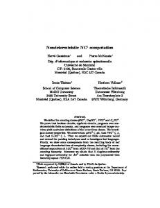
In this section we give some examples of reasoning with |≈S . For this, we use the following notation: Definition 17. Given a context C = {ψ1 , ψ2 , . . . , ψn }, a valuation ν ∈ Λ↓C M is represented by {ψ1 : ν(ψ1 ), ψ2 : ν(ψ2 ), . . . , ψn : ν(ψn )}. The first example illustrates distance-based reasoning in the deterministic case. Example 9. Let us go back to the theory Γ = {p, ¬p, q}, considered in Example 3. As Γ is not classically consistent, everything follows from it in classical logic, including ¬q. Now, consider this theory with respect to the setting S = hMc , dH , Σ, GAtoms i for the standard propositional language, where Mc denotes the standard deterministic matrix and dH is the Hamming (generic) distance (see Example 7). The most plausible valuations in this case are those in which q is true (and so ¬q is false), that is, ∆S (Γ ) = {{p : t, q : t}, {p : f, q : t}}, thus we have that Γ |≈S q while Γ 6|≈S ¬q, as intuitively expected. Note also that in this case Γ 6|≈S p and Γ 6|≈S ¬p. This can be intuitively explained by the fact that p and ¬p are ‘polluted’ by the inconsistency and so they cannot be safely deduced from Γ , even though they are in Γ . In particular, |≈S is not reflexive (but only ‘cautiously reflexive’; see also [2] and the discussion following Definition 21 below). The same conclusions are obtained when dH is replaced by dU . Next, we illustrate distance-based reasoning with non-deterministic semantics. Example 10. Let S = hM, dU ,Σ, GSF i, where M is the Nmatrix considered in Example 1. ↓SF(Γ ) Let Γ = {p, ¬p, q, ¬(p f q)}. Distances to the elements of ΛM are given in Table 1. It follows, then, that ( ) {p : t, ¬p : f, q : t, p f q : f, ¬(p f q) : t}, ∆S (Γ ) = . {p : f, ¬p : t, q : t, p f q : f, ¬(p f q) : t} Thus, for instance, Γ |≈S q and Γ |≈S ¬(p f q), while Γ 6|≈S p and Γ 6|≈S ¬p. Example 11. A reasoner wants to learn as much as possible about a (black-box) circuit, the structure of which is presented in Figure 1. 7

Note that in the deterministic case everything is determined by the values of the atomic formulas, and so the relevant contexts are those that are generated by GAtoms .

11

ν1 ν2 ν3 ν4 ν5

p t t t f f

¬p f f f t t

q t t f t f

pfq t f f f f

¬(p f q) f t t t t

δdU,Σ (·, Γ ) 2 1 2 1 2

Table 1. Distances computations for Example 10.

- G1

in1 in2

- G2

in3

- out

Fig. 1. The malfunction circuit of Example 11.

In this case, G1 and G2 are two AND gates that are faulty or behave unpredictably when both of their input lines are ‘on’.8 After experimenting with the circuit, the reasoner concludes that if one of the input lines is ‘on’ then so is the output line. This situation may be represented by the Nmatrix M of Example 1 as follows: Γ =

©

ª (in1 ∨ in2 ∨ in3 ) → out , ↓SF(Γ )

where out denotes the formula ((in1 f in2 ) f in3 ). The 11 elements of ΛM in Table 2.

ν1 ν2 ν3 ν4 ν5 ν6 ν7 ν8 ν9 ν10 ν11

in1 t t t t t t t f f f f

in2 t t t t t f f t t f f

in3 t t t f f t f t f t f

G1 t t f t f f f f f f f

out t f f f f f f f f f f

δ(ψ1 ) 0 1 1 1 1 1 1 1 1 1 0

δ(ψ2 ) 1 0 1 0 1 1 1 1 1 1 1

δ(Γ ) 0 1 1 1 1 1 1 1 1 1 0

are listed

δ(Γ 0 ) 1 1 2 1 2 2 2 2 2 2 1

↓SF(Γ )

Table 2. Distances to elements of ΛM in Example 11. The following abbreviations are used: G1 = (in1 fin2 ), ψ1 = (in1 ∨in2 ∨in3 ) → out, out = ((in1 fin2 )fin3 ), ψ2 = (in1 fin2 ) ↔ ¬out. Also, δ(·) abbreviates δdU,Σ (ν, ·) for the relevant valuation ν.

8

As noted in Section 2.1, this may happen due to noises on or off chip, variations in the manufacturing process, adversary operations, etc.

12

↓SF(Γ )

Among the valuations in ΛM , two are models of Γ . Thus, by Corollary 1 below, for every setting of the form S = hM, d, f, GSF i, ( © ª ) ν1 = in1 : t, in2 : t, in3 : t, in1 fin2 : t, out : t , © ª , ∆S (Γ ) = modM (Γ ) = ν11 = in1 : f, in2 : f, in3 : f, in1 fin2 : f, out : f so the reasoner may conclude that when all the input lines have the same value, the output line of the circuit preserves this value. Suppose now that the reasoner learns that the value of the output line is always different than the value of the output of G1 . The new situation can be represented by © ª Γ 0 = Γ ∪ (in1 f in2 ) ↔ ¬out . It is easy to verify that Γ 0 is not M-satisfiable anymore, i.e., the new information is inconsistent with the reasoner’s previous knowledge. In such cases the usual |=M entailment is trivialized: everything can be inferred from Γ 0 . This, however, is not the case for |≈S . For instance, when S = hM, dU ,Σ, GSF i, we have that, in the notations of Table 2, © ª   ν = in : t, in : t, in : t, in fin : t, out : t ,  1 1 2 3 1 2      ν = ©in : t, in : t, in : t, in fin : t, out : f ª,   2 1 2 3 1 2 0 © ª ∆S (Γ ) = .  ν4 = in1 : t, in2 : t, in3 : f, in1 fin2 : t, out : f ,      © ª  ν11 = in1 : f, in2 : f, in3 : f, in1 fin2 : f, out : f Using |≈S , the reasoner may still conclude from Γ 0 that if the value of all the input lines is ‘off’, this is also the value of the output line. This shows that |≈S is inconsistencytolerant (see Proposition 7 below). On the other hand, a stronger assertion, that when the values of all input lines coincide the value of the output line is the same, is no longer a valid consequence of Γ 0 . This shows that |≈S is non-monotonic (see Corollary 3 below).

5

General Properties of |≈S

In this section, we consider some basic characteristics of the entailment relations that are induced by our framework. A natural property that one would like to require in this respect, is that models of a satisfiable theory would be closest to that theory among all the relevant valuations. Below, we show that this property holds for all settings with the context generator GSF , and for deterministic settings with the generator GAtoms . Lemma 2. Let S = hM, d, f, Gi. If a) G = GSF , or b) G = GAtoms and M is deterministic, then for every ψ ∈ Γ and for every ν ∈ ΛM , d↓G(Γ ) (ν, ψ) = 0 iff ν ∈ modM (ψ). Proof. Suppose first that d↓G(Γ ) (ν, ψ) = 0. Then there is a valuation µ ∈ modM (ψ) such ↓G(Γ ) that d↓G(Γ ) (ν ↓G(Γ ) , µ↓G(Γ ) ) = 0. Since d↓G(Γ ) is a pseudo distance on ΛM , ν ↓G(Γ ) = ↓G(Γ ) µ . If Γ satisfies condition (a), then µ and ν agree on all the subformulas of ψ, in particular µ(ψ) = ν(ψ), and so ν ∈ modM (ψ). If Γ satisfies condition (b), then µ and ν agree on all the atoms of ψ, and since M is deterministic, µ(ψ) = ν(ψ), so again ν ∈ modM (ψ). For the converse, let ν ∈ modM (ψ). Then again, as d↓G(Γ ) is a pseudo ↓G(Γ ) distance on ΛM , d↓G(Γ ) (ν ↓G(Γ ) , ν ↓G(Γ ) ) = 0 and thus d↓G(Γ ) (ν, ψ) = 0. u t 13

Corollary 1. Let S = hM, d, f, Gi be a setting such that either (a) G = GSF , or (b) G = GAtoms and M is deterministic. Then a theory Γ is M-satisfiable iff ∆S (Γ ) = modM (Γ ). Proof. Suppose first that ∆S (Γ ) = modM (Γ ). By Lemma 1 we have that modM (Γ ) is not empty, and so Γ is M-satisfiable. For the converse, note that by Lemma 2 we have ↓G(Γ ) that δd,f (ν, Γ ) = 0 iff ν ∈ modM (Γ ). Thus, ↓G(Γ )

ν ∈ modM (Γ ) ⇐⇒ ⇐⇒ ⇐⇒

δd,f 9

(ν, Γ ) = 0, ↓G(Γ )

∀µ ∈ ΛM δd,f

↓G(Γ )

(ν, Γ ) ≤ δd,f

(µ, Γ ),

ν ∈ ∆S (Γ ).

u t

The next example shows that the above corollary does not hold for the context generator GAtoms and an arbitrary non-deterministic Nmartix (i.e., when condition (b) of Lemma 2 is relaxed). Example 12. Let S = hM, dU ,Σ, GAtoms i, where M is the Nmatrix considered in Example 1, and Γ = {p, q, p f q}. This theory is clearly M-satisfiable, and © ª modM (Γ ) = {p : t, q : t, pfq : t} . However, as the relevant context in this case is Atoms(Γ ) = {p, q}, we have that © ª ∆S (Γ ) = {p : t, q : t, pfq : t}, {p : t, q : t, pfq : f } . It follows, therefore, that in the general case using the context generator GSF is more appropriate than using GAtoms . In what follows we shall thus concentrate on settings of the form S = hM, d, f, GSF i. Henceforth, we shall refer to a setting as a triple S = hM, d, f i, assuming that the context generator is GSF . The next property relates standard and distance-based entailments for Nmatrices. Proposition 6. For every setting S = hM, d, f i, if Γ |≈S ψ then Γ |=M ψ. Moreover, if Γ is M-satisfiable, then Γ |≈S ψ iff Γ |=M ψ. Proof. Follows from Corollary 1 and the fact that if Γ is not M-satisfiable then Γ |=M ψ for every ψ. u t It follows that |≈S coincides with |=M for M-consistent theories. In contrast to |=M , however, |≈S tolerates inconsistency and has some non-monotonic characteristics. We discuss these properties below. Definition 18 (independence). Two theories Γ1 and Γ2 are called independent if Atoms(Γ1 ) ∩ Atoms(Γ2 ) = ∅. Proposition 7 (paraconsistency). For every Γ and every ψ such that Γ and {ψ} are independent, Γ |≈S ψ iff ψ is an M-tautology. Proof. One direction is clear: if ψ is an M-tautology, then for every ν ∈ ∆S (Γ ), ν(ψ) = t and so Γ |≈S ψ. For the converse, suppose that ψ is not an M-tautology. Then there is some M-valuation σ, such that σ(ψ) = f . Let ν ∈ ∆S (Γ ). If ν(ψ) = f , we are done. Otherwise, since Γ and {ψ} are independent, there is an M-valuation µ such that µ(ϕ) = ν(ϕ) for every ϕ ∈ SF(Γ ) and µ(ϕ) = σ(ϕ) for ϕ ∈ SF(ψ). Since S is unbiased ↓SF(Γ ) (Proposition 4), d↓SF(Γ ) (ν, γ) = d↓SF(Γ ) (µ, γ) for every γ ∈ Γ . Thus, δd,f (ν, Γ ) = ↓SF(Γ )

δd,f 9

(µ, Γ ) and µ ∈ ∆S (Γ ). But µ(ψ) = σ(ψ) = f and so Γ 6|≈S ψ.

Note that the direction ⇐ follows from the fact that Γ is M-satisfiable.

14

u t

Corollary 2 (non-explosion). For every Γ there is a ψ s.t. Γ 6|≈S ψ. Proof. Given a set Γ of formulas, let p ∈ Atoms \ SF(Γ ). As Γ and {p} are independent, by Proposition 7, Γ 6|≈S p. u t Note 3. It is important to note that Corollary 2 indicates that every theory in L is non-explosive with respect to |≈S . This property is not obvious even for logics that admit non-trivial reasoning in the presence of inconsistency. For instance, in the Logics of Formal Inconsistency (LFIs) [16, 17], theories of the form {p, ¬p} are non-explosive, but, e.g., the theory {◦p, p, ¬p} entails every well-formed formula. Corollary 2 can be strengthen for settings with a classical negation operator: Definition 19. An Nmartix M = h{t, f }, {t}, Oi is with negation, if there is a unary function ¬ e in O such that ¬ e (t) = {f } and ¬ e (f ) = {t}. A setting S = hM, d, f i is with negation if its Nmatrix M is with negation. Proposition 8. Let S be a setting with negation. Then for every Γ and every ψ, if Γ |≈S ψ then Γ 6|≈S ¬ψ. Proof. Suppose that there is a formula ψ such that Γ |≈S ψ and Γ |≈S ¬ψ. Then ∆S (Γ ) ⊆ modM (ψ) and ∆S (Γ ) ⊆ modM (¬ψ). But modM (ψ) ∩ modM (¬ψ) = ∅, and so ∆S (Γ ) = ∅, a contradiction to the fact that ∆S (Γ ) 6= ∅ for every Γ . u t It follows, then, that according to |≈S , the set of conclusions cannot be contradictory even when the set of premises is not M-consistent. Corollary 3 (non-monotonicity). Let S = hM, d, f i be a setting with negation. Then |≈S is non-monotonic. Proof. Clearly, p |≈S p and ¬p |≈S ¬p. By Proposition 8, on the other hand, either p, ¬p 6|≈S p or p, ¬p 6|≈S ¬p (or both). Hence, the set of conclusions does not monotonically grow with respect to the size of the premises, and so |≈S is non-monotonic. u t In spite of Corollary 3, even for settings with negation, one may specify conditions under which the entailment relations have some monotonic characteristics. Next, we consider such cases. For this,we need the following property of aggregation functions: Definition 20 (hereditary functions). An aggregation function f is hereditary, if for every x1 , . . . , xn , y1 , . . . , yn , the fact that f ({x1 , . . . , xn }) < f ({y1 , . . . , yn }) implies that for every z1 , . . . , zm , f ({x1 , . . . , xn , z1 , . . . , zm }) < f ({y1 , . . . , yn , z1 , . . . , zm }). Example 13. Summation is hereditary, while the maximum and the voting functions are not. For instance, 12 = majority({0, 1}) < majority({1, 1}) = 1, but 1 = majority({0, 1, 1}) = majority({1, 1, 1}) = 1. The following proposition shows that in light of new information that is unrelated to the premises, previously drawn conclusions should not be retracted.10 10

This type of monotonicity is a kind of rational monotonicity, considered in [30].

15

Proposition 9 (rational monotonicity). Let S = hM, d, f i be a setting in which f is hereditary. If Γ |≈S ψ, then Γ, φ |≈S ψ for every formula φ such that Γ ∪ {ψ} and {φ} are independent. Proof. Let Γ = {ψ1 , . . . , ψn } and let µ ∈ ΛM , so that µ(ψ) = f . As Γ |≈S ψ, µ 6∈ ∆S (Γ ), ↓SF(Γ ) ↓SF(Γ ) so there is a valuation ν ∈ ∆S (Γ ) with δd,f (ν, Γ ) < δd,f (µ, Γ ), that is, f ({d↓SF(Γ ) (ν, ψ1 ), . . . , d↓SF(Γ ) (ν, ψn )}) < f ({d↓SF(Γ ) (µ, ψ1 ), . . . , d↓SF(Γ ) (µ, ψn )}). Now, as Γ |≈S ψ, it follows that ν(ψ) = t, and as Atoms(Γ ∪ {ψ}) ∩ Atoms({φ}) = ∅, one can easily define an M-valuation σ such that σ(ϕ) = ν(ϕ) for every ϕ ∈ SF(Γ ∪ {ψ}) and σ(ϕ) = µ(ϕ) for every ϕ ∈ SF({φ}). By Proposition 4, and since f is hereditary, we have: ↓SF(Γ )

δd,f

(σ, Γ ∪ {φ}) = f ({d↓SF(Γ ) (σ, ψ1 ), . . . , d↓SF(Γ ) (σ, ψn ), d↓SF(Γ ) (σ, φ)}) = f ({d↓SF(Γ ) (ν, ψ1 ), . . . , d↓SF(Γ ) (ν, ψn ), d↓SF(Γ ) (µ, φ)}) ↓SF(Γ )

< f ({d↓SF(Γ ) (µ, ψ1 ), . . . , δd,f ↓SF(Γ )

= δd,f

(µ, ψn ), d↓SF(Γ ) (µ, φ)})

(µ, Γ ∪ {φ})

Thus, for every µ ∈ ΛM such that µ(ψ) = f , there is some σ ∈ ΛM such that σ(ψ) = t ↓SF(Γ ) ↓SF(Γ ) and δd,f (σ, Γ ∪ {φ}) < δd,f (µ, Γ ∪ {φ}). It follows that the elements of ∆S (Γ ∪ {φ}) must satisfy ψ, and so Γ, φ |≈S ψ. u t Note 4. As the following example shows, heredity is indeed necessary in Proposition 9 for assuring rational monotonicity, even for independent premises: Example 14. Let S = hMc , dU , majorityi and Γ = {p, ¬p, q}. Then © ª ∆S (Γ ) = {p : t, q : t}, {p : f, q : t} , and so Γ |≈S q. Now, let Γ 0 = Γ ∪ {r}. We have, ( ) {p : t, q : t, r : f }, {p : t, q : t, r : t}, {p : t, q : f, r : t}, ∆S (Γ 0 ) = , {p : f, q : t, r : f }, {p : f, q : t, r : t}, {p : f, q : f, r : t} so this time Γ 0 6|≈S q. The discussion above, on the non-monotonicity of |≈S , brings us to the question to what extent these entailments can be considered as consequence relations. Definition 21 (consequence relations). A Tarskian consequence relation [41] for a language L is a binary relation ` between sets of formulas of L and formulas of L that satisfies the following conditions: Reflexivity: if ψ ∈ Γ , then Γ ` ψ. Monotonicity: if Γ ` ψ and Γ ⊆ Γ 0 , then Γ 0 ` ψ. Transitivity: if Γ ` ψ and Γ 0 , ψ ` φ, then Γ, Γ 0 ` φ. Proposition 10. [12] For every Nmartix M, |=M is a Tarskian consequence relation. 16

As opposed to |=M , entailments of the form |=S are not consequence relations, since, as follows from Example 10 and Corollary 3, they are neither reflexive nor monotonic. To see that transitivity may not hold either, consider a propositional language with negation and the setting S = hMc , d, f i for any pseudo distance d and aggregation function f . If p, ¬p 6|≈S q, transitivity does not hold, since by Proposition 6, p |≈S ¬p → q and ¬p, ¬p → q |≈S q; Otherwise, if p, ¬p |≈S q, then by Proposition 8, p, ¬p 6|≈S ¬q, and this, together with the facts that p |≈S ¬p → ¬q and ¬p, ¬p → ¬q |≈S ¬q (Proposition 6 again) provide a counterexample for transitivity. In the context of non-monotonic reasoning, however, it is usual to consider the following weaker conditions that guarantee a ‘proper behaviour’ of nonmonotonic entailments in the presence of inconsistency (see, e.g., [4, 27, 30, 34]): Definition 22 (cautious consequence relations). A cautious consequence relation for L is a relation |∼ between sets of L-formulas and L-formulas, that satisfies the following conditions: Cautious Reflexivity (w.r.t. M): if Γ is M-satisfiable and ψ ∈ Γ , then Γ |∼ ψ. Cautious Monotonicity [22]: if Γ |∼ ψ and Γ |∼ φ, then Γ, ψ |∼ φ. Cautious Transitivity [27]: if Γ |∼ ψ and Γ, ψ |∼ φ, then Γ |∼ φ. Proposition 11. Let S = hM, d, f i be a setting where f is hereditary. Then |≈S is a cautious consequence relation. Proof. Cautious reflexivity follows from Proposition 6. The proofs for cautious monotonicity and cautious transitivity are an adaptation of the ones for the deterministic case (see [2]): For cautious monotonicity, let Γ = {γ1 , . . . , γn } and suppose that Γ |≈S ψ, Γ |≈S φ, and ν ∈ ∆S (Γ ∪ {ψ}). We show that ν ∈ ∆S (Γ ) and since Γ |≈S φ this implies that ν ∈ modM ({φ}). Indeed, if ν ∈ / ∆S (Γ ), there is a valuation µ ∈ ∆S (Γ ) so that δd,f (µ, Γ ) < δd,f (ν, Γ ), i.e., f ({d(µ, γ1 ), . . . , d(µ, γn )}) < f ({d(ν, γ1 ), . . . , d(ν, γn )}). Also, as Γ |≈S ψ, µ ∈ modM ({ψ}), thus d(µ, ψ) = 0. By these facts, then, δd,f (µ, Γ ∪ {ψ}) = f ({d(µ, γ1 ), . . . , d(µ, γn ), 0}) < f ({d(ν, γ1 ), . . . , d(ν, γn ), 0}) ≤ f ({d(ν, γ1 ), . . . , d(ν, γn ), d(ν, ψ)}) = δd,f (ν, Γ ∪ {ψ}), a contradiction to ν ∈ ∆S (Γ ∪ {ψ}). For cautious transitivity, let again Γ = {γ1 , . . . , γn } and assume that Γ |≈S ψ, Γ, ψ |≈S φ, and ν ∈ ∆S (Γ ). We have to show that ν ∈ modM ({φ}). Indeed, since ν ∈ ∆S (Γ ), for all µ ∈ ΛM , f ({d(ν, γ1 ), . . . , d(ν, γn )}) ≤ f ({d(µ, γ1 ), . . . , d(µ, γn )}). Moreover, since Γ |≈S ψ, ν ∈ modM ({ψ}), and so d(ν, ψ) = 0 ≤ d(µ, ψ). It follows, then, that for every µ ∈ ΛM , δd,f (ν, Γ ∪ {ψ}) = f ({d(ν, γ1 ), . . . , d(ν, γn ), d(ν, ψ)}) ≤ f ({d(µ, γ1 ), . . . , d(µ, γn ), d(ν, ψ)}) ≤ f ({d(µ, γ1 ), . . . , d(µ, γn ), d(µ, ψ)}) = δd,f (µ, Γ ∪ {ψ}). Thus, ν ∈ ∆S (Γ ∪ {ψ}), and since Γ, ψ |≈S φ, necessarily ν ∈ modM ({φ}).

u t

Regarding the computability of our entailments, we show that in most of the practical cases entailment checking is decidable. 17

Definition 23 (computable settings). A setting S = hM, d, f i is computable, if f is computable, and there is an algorithm that computes d↓C (µ, ν) for every context C and every µ, ν ∈ Λ↓C M. Note 5. Clearly, all the distance and aggregation functions considered in this paper are computable. Yet, as the following example shows, this is not always the case. Let L = {∧} be a propositional language and L a first-order language with a constant c, a unary function g and a binary relation R. Consider the following one-to-one mapping Θ from L-formulas to L-formulas: every symbol s in L is associated with an atomic formula ps in L, and every L-formula ψ is mapped to the L-formula Θ(ψ), obtained by taking the conjunction of all the atomic formulas to which the symbols of ψ are mapped. For instance, the formula ∀x1 ∀x2 R(x1 , x2 ) is mapped to p∀ ∧ px1 ∧ p∀ ∧ px2 ∧ pR ∧ p( ∧ px1 ∧ p, ∧ px2 ∧ p) . A formula ψ in L is called proper if there is an L-formula ψ 0 s.t. ψ = Θ(ψ 0 ). Now, consider the following generic pseudo distance:  0 if ν = µ,    ↓SF(ψ) 1 if ν 6= µ and there is a proper ψ such that ν, µ ∈ ΛM d(ν, µ) = −1  and Θ (ψ) is satisfiable,   2 otherwise. Since SF(ψ) 6= SF(φ) whenever ψ 6= φ, the pseudo distance above is well defined. Now, as the satisfiability problem for L-formulas is undecidable, d is not computable. Proposition 12 (decidability). If S is computable then the question whether Γ |≈S ψ is decidable. Proof. Suppose that S is a computable setting. By Definition 21, in order to check whether Γ |≈S ψ, one has to check whether ∆S (Γ ) ⊆ modM (ψ). For decidability, we show that this condition, which is based on infinite sets of valuations, can be reduced to an equivalent condition in terms of finite sets of partial valuations. For this, we denote ↓C by mod↓C | µ ∈ modM (ψ)}. Next, we extend the notions of distance M (ψ) the set {µ between a valuation and a formula, and distance between a valuation and a theory, to partial valuations as follows: for every context C such that SF(Γ ) ⊆ C, define, for every ν ∈ Λ↓C M and every ψ ∈ Γ : – d↓SF(Γ ) (ν, ψ) = ( min{d↓SF(Γ ) (ν ↓SF(Γ ) , µ↓SF(Γ ) ) | µ ∈ mod↓C M (ψ)} ↓SF(Γ )

1 + max{d↓SF(Γ ) (µ1 ↓SF(Γ )

– δd,f

↓SF(Γ )

, µ2

if mod↓C M (ψ) 6= ∅,

) | µ1 , µ2 ∈ Λ↓C M } otherwise.

(ν, Γ ) = f ({d↓SF(Γ ) (ν, ψ1 ), . . . , d↓SF(Γ ) (ν, ψn )}).

Note that since all the partial valuations involved in the definitions above are defined on finite contexts, there are finitely many such valuations to check, and so d↓SF(Γ ) (ν, ψ) ↓SF(Γ ) and δd,f (ν, Γ ) are computable for every ν ∈ Λ↓C M . Now, consider the following set of partial valuations on C: (© ª ↓SF(Γ ) ↓SF(Γ ) ν ∈ Λ↓C (ν, Γ ) ≤ δd,f (µ, Γ ) if Γ 6= ∅, ↓C M | ∀µ ∈ ΛM δd,f ∆S (Γ ) = Λ↓C otherwise. M ↓C Clearly, ∆↓C S (Γ ) and modM (ψ) are computable for any context C. Decidability now fol↓SF(Γ∪{ψ}) ↓SF(Γ∪{ψ}) lows from the fact that ∆S (Γ ) ⊆ modM (ψ) iff ∆S (Γ ) ⊆ modM (ψ). u t

18

6

Particular Cases of Reasoning with |≈S

In this section we consider in greater details some particular instances of distance-based entailments with drastic settings, that is, settings with a drastic distance (see Example 5). In particular, we investigate their relations to other reasoning and satisfiability problems. 6.1

Drastic Settings with Range-Restricted Functions

Definition 24 (range-restricted functions). An aggregation function f is called range restricted , if f ({x1 , . . . , xn }) ∈ {x1 , . . . , xn }. Example 15. max is a range-restricted function, while Σ and vote k are not rangem restricted. Proposition 13. Let S = hM, dU , f i be a drastic setting in which f is range restricted. Let Γ be a set of formulas that is not M-satisfiable. Then Γ |≈S ψ iff ψ is an Mtautology. Proof. Let µ ∈ ΛM . As Γ = {ϕ1 , . . . , ϕn } is not M-satisfiable, µ is not a model of Γ , ↓SF(Γ ) and so there is some ϕj ∈ Γ such that dU (µ, ϕj ) = 1. Moreover, for every ϕi ∈ Γ we ↓SF(Γ ) have that dU (µ, ϕi ) ∈ {0, 1} and so, since f is range-restricted, ↓SF(Γ )

δdU,f

↓SF(Γ )

(µ, Γ ) = f ({dU

↓SF(Γ )

(µ, ϕ1 ), . . . , dU

(µ, ϕn )}) = 1.

This shows that all the valuations in ΛM are equally distant from Γ and so ∆S (Γ ) = ΛM . Thus, Γ |≈S ψ iff ∆S (Γ ) ⊆ modM (ψ), iff modM (ψ) = ΛM , iff ψ is a tautology. u t Corollary 4. Let S be a drastic setting with a range-restricted aggregation function, and suppose that Γ |≈S ψ. Then: – if Γ is M-satisfiable, Γ |=M ψ – if Γ is not M-satisfiable, ψ is an M-tautology. Proof. The first case follows from Proposition 6 and the second case follows from Proposition 13. u t It follows that reasoning with drastic settings and range restricted functions has a somewhat ‘crude nature’, and in practice we hardly deviate from the basic entailment: the set of conclusions coincides with that of the basic entailment, unless the set of premises is contradictory, in which case only tautologies are entailed. 6.2

Drastic Settings with Additive Functions

Definition 25 (additive functions). An aggregation function f is called additive, if for any non-empty multiset S it can be represented as f (S) = g(|S|) · Σx∈S x, for some function g : N+ → R+ . Example 16. The summation (respectively, the average) function is additive, where g is uniformly 1 (respectively, where g(n) = n1 ). 19

The characteristics of entailments induced by drastic settings with additive functions are completely different than those of entailments that are obtained by drastic settings with range-restricted functions. As we show next, the former are closely related to the maximal satisfiability problem: Definition 26 (max-SAT). Let SATM (Γ ) be the set of all the M-satisfiable subsets of Γ . The set mSATM (Γ ) of the maximally M-satisfiable subsets of Γ consists of all the elements Υ ∈ SATM (Γ ) such that |Υ 0 | ≤ |Υ | for every Υ 0 ∈ SATM (Γ ). Note 6. Clearly, mSATM (Γ ) is nonempty whenever Γ contains an M-satisfiable element, so in this case |Υ | ≥ 1 for all Υ ∈ mSATM (Γ ). Also, all the elements in mSATM (Γ ) are of the same size. Proposition 14. Let S = hM, dU , f i be a drastic setting with an additive function f . Then for every theory Γ , ( {ν ∈ modM (Υ ) | Υ ∈ mSATM (Γ )} if mSATM (Γ ) 6= ∅, ∆S (Γ ) = ΛM otherwise. Proof. Consider a theory Γ = {ψ1 , . . . , ψn }, and assume first that mSATM (Γ ) 6= ∅. Since ↓SF(Γ ) S is drastic, for every ψ ∈ Γ and every ν ∈ ΛM , dU (ν, ψ) = 0 if ν ∈ modM (ψ) and ↓SF(Γ ) otherwise dU (ν, ψ) = 1. Now, since f is additive, we have that ↓SF(Γ )

δdU,f

↓SF(Γ )

(ν, Γ ) = f {dU

↓SF(Γ )

(ν, ψ1 ), . . . , dU

↓SF(Γ ) (dU (ν, ψ1 )

(ν, ψn )} ↓SF(Γ )

= g(n) · + . . . + dU = g(n) · |{ψ ∈ Γ | ν ∈ / modM (ψ)}|.

(ν, ψn ))

Thus, ν ∈ ∆S (Γ ) iff the set {ψ ∈ Γ | ν ∈ / modM (ψ)} is minimal in its size, iff {ψ ∈ Γ | ν ∈ modM (ψ)} is maximal in its size, iff this set belongs to mSATM (Γ ). Now assume that mSATM (Γ ) = ∅. In this case none of the formulas in Γ is Msatisfiable (see Note 6). Thus, as ↓SF(Γ )

MdU (Γ ) = max{dU

↓SF(Γ )

(µ1

↓SF(Γ )

, µ2

) | µ1 , µ2 ∈ ΛM } = 1,

we have that for every ν ∈ ΛM , ↓SF(Γ )

δdU,f

↓SF(Γ )

(ν, Γ ) = f {dU

↓SF(Γ )

(ν, ψ1 ), . . . , dU

↓SF(Γ ) (dU (ν, ψ1 )

(ν, ψn )} ↓SF(Γ )

= g(n) · + . . . + dU = g(n) · n · (1 + MdU (Γ )) = 2n · g(n).

(ν, ψn ))

Thus, all the elements in ΛM are equally distant from Γ , and so ∆S (Γ ) = ΛM .

u t

Corollary 5. Let S be a drastic setting with an additive aggregation function. If mSATM (Γ ) is non-empty, then Γ |≈S ψ iff Γ 0 |=M ψ for every Γ 0 ∈ mSATM (Γ ). Proof. Suppose for contradiction that Γ |≈S ψ but there is some Γ 0 ∈ mSATM (Γ ) such that Γ 0 6|=M ψ. Then there is an M-valuation ν, such that ν ∈ modM (Γ 0 ) and ν 6∈ modM (ψ). By Proposition 14, ν ∈ ∆S (Γ ). Thus, ∆S (Γ ) 6⊆ modM (ψ), and so Γ 6|≈S ψ. For the converse, let ν ∈ ∆S (Γ ). Again, by Proposition 14 there is some Γ 0 ∈ mSATM (Γ ) such that ν ∈ modM (Γ 0 ). As Γ 0 |=M ψ, ν(ψ) = t, which implies that Γ |≈S ψ. u t 20

Example 17. By taking S = hMc , dU , Σi in the last corollary, we get that reasoning with summation of drastic distances is equivalent to checking classical entailments from the maximally consistent subsets of the premises. The following result should be compared with Proposition 9: Proposition 15 (rational monotonicity). Let S be a drastic setting with an additive aggregation function, and let Γ be a theory such that mSATM (Γ ) is not empty. If Γ |≈S ψ, then Γ, φ |≈S ψ for every formula φ 6∈ Γ for which there is an element Υ ∈ mSATM (Γ ) such that Υ ∪ {φ} is M-satisfiable. For the proof of Proposition 15 we need the following lemma. Lemma 3. Let Γ be a theory such that mSATM (Γ ) is not empty, and let Γ 0 ∈ mSATM (Γ ). Suppose that ϕ 6∈ Γ and Γ 0 ∪ {ϕ} is M-satisfiable. Then: mSATM (Γ ∪ {ϕ}) = {Υ ∪ {ϕ} | Υ ∈ mSATM (Γ ) and Υ ∪ {ϕ} is M-satisfiable}. Proof. Let n be the size of the elements of mSATM (Γ ). By Note 6, Γ 0 is also of size n. Now, let Ω ∈ mSATM (Γ ∪ {ϕ}). Suppose for a contradiction that Ω is not of the form Υ ∪ {ϕ}, where Υ ∈ mSATM (Γ ). Since Ω ⊆ Γ ∪ {ϕ}, either Ω ⊆ Γ or Ω is of the form Υ ∪ {ϕ}, where Υ ⊆ Γ but Υ 6∈ mSATM (Γ ). Suppose first that Ω ⊆ Γ . Then since Ω ∈ SATM (Γ ), it must be of size at most n. In this case, Γ 0 ∪ {ϕ} ∈ SATM (Γ ∪ {ϕ}) is of size n + 1, in contradiction to the maximality of Ω. In the second case, where Ω is of the form Υ ∪ {ϕ} and Υ ⊆ Γ but Υ 6∈ mSATM (Γ ), we have that Υ ∪ {ϕ} is of size at most n (since the size of Υ is less than n), while there is an M-satisfiable set Γ 0 ∪ {ϕ} of size n + 1. This contradicts the fact that Ω ∈ mSATM (Γ ∪ {ϕ}). For the converse, let Υ ∈ mSATM (Γ ) such that Υ ∪{ϕ} is M-satisfiable. Then Υ is of size n. Suppose for a contradiction that Υ ∪ {ϕ} 6∈ mSATM (Γ ∪ {ϕ}). Then the elements of mSATM (Γ ∪ {ϕ}) are of size at least n + 2, and so there must be some Ω ∈ SATM (Γ ) of size n + 1. This contradicts our assumption about the size of elements of mSATM (Γ ). u t Proof (of Proposition 15). Let ν ∈ ∆S (Γ ∪ {φ}). By Proposition 14, ν ∈ modM (Υ ) for some Υ ∈ mSATM (Γ ∪ {φ}). By Lemma 3, Υ = Υ 0 ∪ {φ}, where Υ 0 ∈ mSATM (Γ ). In particular, then, ν ∈ modM (Υ 0 ), and by Proposition 14 again, ν ∈ ∆S (Γ ). But Γ |≈S ψ, thus ν(ψ) = t, and so Γ, φ |≈S ψ. u t As a particular case of Proposition 15, we get that independence (Definition 18) is a sufficient syntactic condition for rational monotonicity. Corollary 6. Let S be a drastic setting with an additive aggregation function. If Γ |≈S ψ then Γ, φ |≈S ψ for every M-satisfiable formula φ that is independent of Γ . Proof. If φ is M-satisfiable and independent of Γ , then in particular φ 6∈ Γ and for every Υ ∈ mSATM (Γ ), Υ ∪ {φ} is M-satisfiable. Indeed, assuming that ν ∈ modM (Υ ) and µ ∈ modM (φ), it easy to verify that σ, defined by σ(γ) = ν(γ) for every γ ∈ SF(Υ ) ↓SF(Υ∪{ψ}) and σ(γ) = µ(γ) for every γ ∈ SF(φ), is a well-defined valuations in ΛM that M-satisfies Υ ∪ {φ}. The claim now follows from Proposition 15. u t 21

6.3

Drastic Settings with Voting Functions

Next, we consider settings of the form S = hM, dU , vote k i, where the induced entailm k ments are determined by a quorum of at least d m e of the ‘votes’ (recall Example 6). Definition 27. Denote by k size is at least d m |Γ |e.

k m SATM (Γ )

the set of all the M-satisfiable subsets of Γ whose

Proposition 16. Let S = hM, dU , vote k i and let Γ be a theory that is not M-satisfiable. m Then: ( {ν ∈ modM (Υ ) | Υ ∈ mk SATM (Γ )} if mk SATM (Γ ) 6= ∅, ∆S (Γ ) = ΛM otherwise. Proof. To reduce notation complexity, we omit in what follows the subscripts in δd↓C . U ,vote k m

Suppose that Γ is not M-satisfiable. Then δ ↓SF(Γ ) (ν, Γ ) ≥ 21 for all ν ∈ ∆S (Γ ). Assume first that mk SATM (Γ ) is not empty. Then there is µ ∈ ΛM for which δ ↓SF(Γ ) (µ, Γ ) = 21 . Thus, for every ν ∈ ΛM , ν ∈ ∆S (Γ ) iff δ ↓SF(Γ ) (ν, Γ ) = 21 , iff there is some Υ ∈ mk SATM (Γ ) such that ν ∈ modM (Υ ). If mk SATM (Γ ) is empty, then for all ν ∈ ΛM , δ ↓SF(Γ ) (ν, Γ ) = 1, and so ∆S (Γ ) = ΛM . u t The proof of the next corollary is similar to that of Corollary 5. Corollary 7. Let S = hM, dU , vote k i. If Γ is not M-satisfiable and m non-empty, then Γ |≈S ψ iff Γ 0 |=M ψ for every Γ 0 ∈ mk SATM (Γ ).

k m SATM (Γ )

is

Reasoning with settings of the form S = hM, dU , vote k i is therefore summarized as m follows: For every theory Γ and formula ψ, – if Γ is M-satisfiable, then Γ |≈S ψ iff Γ |=M ψ – if Γ is not M-satisfiable and Γ 0 ∈ mk SATM (Γ ) – if Γ is not M-satisfiable and

7

k m SATM (Γ )

k m SATM (Γ )

6= ∅, then Γ |≈S ψ iff Γ 0 |=M ψ for all

= ∅, then Γ |≈S ψ iff ψ is an M-tautology.

Summary and Future Work

In this paper, we introduced a general framework for reasoning with uncertainty, in which non-deterministic semantics is augmented with distance-based considerations. This allows to capture different scenarios in which inconsistency and incompleteness arise, as demonstrated in the example of the malfunctioning device. Our framework is a conservative extension of the deterministic case, thus when the underlying matrix is deterministic, standard distance-based approaches to non-monotonic reasoning are reconstructed. It is shown, moreover, that some particular instances of the entailments that are obtained by our framework have strong ties to well-known SAT problems. There are several directions for future work. One important line of research is to consider Nmatrices with finitely many truth values (rather than the two-valued Nmatrices considered here). Such a generalization is motivated e.g. in [11], where Belnap’s 22

four-valued framework [14] is extended to four-valued Nmatrices, and is applied for information integration. Another generalization is related to the way that non-determinism is incorporated. As opposed to the dynamic version used here, according to static non-deterministic semantics, defined in [10], the choice of ν(¦(ψ1 , . . . , ψn )) out of the possible options in e ¦(ν(ψ1 ), . . . , ν(ψn )) is made globally and it is system-wide. Thus, the interpretation of ¦ is a function that is determined before any computation begins. This function is a ‘determinization’ of the non-deterministic interpretation e ¦ and it is applied in computing the value of any formula under the given valuation. This limits non-determinism, but still leaves the freedom of choosing the above function among all options in the nondeterministic interpretation e ¦ of ¦. Static semantics gives rise to interesting situations that are inherently incomplete, such as when the structure of the electrical circuit in our canonical example is not known to the reasoner. Finally, for real-life applications, extensions to first-order languages and beyond has to be addressed. In the context of belief revision and (distance-based) database integration it is usual to deal with this by grounding the theory and so reducing everything back to the propositional case. This is, however, time and space consuming. An extension of the framework of Nmatrices to languages with quantifiers has been studied, e.g., in [13]. A similar approach in our case should involve distances not only between valuations, but also between first-order structures. This is another subject for future work.

References 1. M. Arenas, L. Bertossi, and J. Chomicki. Answer sets for consistent query answering in inconsistent databases. Theory and Practice of Logic Programming, 3(4–5):393–424, 2003. 2. O. Arieli. Distance-based paraconsistent logics. International Journal of Approximate Reasoning, 48(3):766–783, 2008. 3. O. Arieli. Reasoning with prioritized information by iterative aggregation of distance functions. Journal of Applied Logic, 6(4):589–605, 2008. 4. O. Arieli and A. Avron. General patterns for nonmonotonic reasoning: from basic entailments to plausible relations. Logic Journal of the IGPL, 8(2):119–148, 2000. 5. O. Arieli, M. Denecker, and M. Bruynooghe. Distance semantics for database repair. Annals of Mathematics and Artificial Intelligence, 50(3–4):389–415, 2007. 6. O. Arieli, M. Denecker, B. Van Nuffelen, and M. Bruynooghe. Computational methods for database repair by signed formulae. Annals of Mathematics and Artificial Intelligence, 46(1–2):4–37, 2006. 7. O. Arieli and A. Zamansky. Reasoning with uncertainty by Nmatrix–Metric semantics. In Proc. 15th Workshop on Logic, Language, Information and Computation (WoLLIC’08), LNAI 5110, pages 69–82. Springer, 2008. 8. O. Arieli and A. Zamansky. Some simplified forms of reasoning with distance-based entailments. In Proc. 21st Canadian AI, LNAI 5032, pages 36–47. Springer, 2008. 9. A. Avron. Non-deterministic semantics for logics with a consistency operator. International Journal of Approximate Reasoning, 45:271–287, 2007. 10. A. Avron and B. Konikowska. Multi-valued calculi for logics based on non-determinism. Logic Journal of the IGPL, 13(4):365–387, 2005. 11. A. Avron, B. Konikowska, and J. Ben-Naim. Processing information from a set of sources. to appear in Trends in Logic, 27, 2008. 12. A. Avron and I. Lev. Non-deterministic multi-valued structures. Journal of Logic and Computation, 15:241–261, 2005.

23

13. A. Avron and A. Zamansky. Many-valued non-deterministic semantics for first-order logics of formal inconsistency. In S. Aguzzoli et al., editor, Algebraic and Proof-theoretic Aspects of Non-classical Logics, LNAI 4460, pages 1–24. Springer, 2007. 14. N. Belnap. A useful four-valued logic. Modern uses of multiple-valued logic, 27:5–37, 1977. 15. J. Ben Naim. Lack of finite characterizations for the distance-based revision. In Proc. KR’06, pages 239–248. AAAI Press, 2006. 16. W. Carnielli, M. Esteban, and J. Marcos. Logics of formal inconsistency. In D. M. Gabbay and F. Guenthner, editors, Handbook of Philosophical Logic, volume 14, pages 1–95. Springer, 2007. Seond edition. 17. W. Carnielli and J. Marcos. A taxonomy of C-systems. In W. A. Carnielli, M. E. Coniglio, and I. D’Ottaviano, editors, Paraconsistency: The Logical Way to the Inconsistent, number 228 in Lecture Notes in Pure and Applied Mathematics, pages 1–94. Marcel Dekker, 2002. 18. J. Chomicki. Consistent query answering: Five easy pieces. In Proc. ICDT’07, LNCS 4353, pages 1–17. Springer, 2007. 19. J. Chomicki and J. Marchinkowski. Minimal-change integrity maintenance using tuple deletion. Information and Computation, 197(1–2):90–121, 2005. 20. M. Dalal. Investigations into a theory of knowledge base revision. In Proc. AAAI’88, pages 475–479. AAAI Press, 1988. 21. D. Dubois and H. Prade. Belief change and possibility theory. In P. G¨ ardenfors, editor, Belief Revision, pages 142–182. Cambridge Press, 1992. 22. D. Gabbay. Theoretical foundation for non-monotonic reasoning, Part II: Structured nonmonotonic theories. In Proc. SCAI’91. IOS Press, 1991. 23. S. Gottwald. A Treatise on Many-Valued Logics, Studies in Logic and Computation, volume 9. Research Studies Press, Baldock, 2001. 24. A. Grove. Two modellings for theory change. Journal of Philosophical Logic, 17:157–180, 1988. 25. S. Konieczny, J. Lang, and P. Marquis. Distance-based merging: a general framework and some complexity results. In Proc. KR’02, pages 97–108. Morgan Kaufmann Publishers, 2002. 26. S. Konieczny and R. Pino P´erez. Merging information under constraints: a logical framework. Logic and Computation, 12(5):773–808, 2002. 27. S. Kraus, D. Lehmann, and M. Magidor. Nonmonotonic reasoning, preferential models and cumulative logics. Artificial Intelligence, 44(1–2):167–207, 1990. 28. C. Lafage and J. Lang. Logical representation of preference for group decision making. In Proc. KR’2000, pages 457–468. Morgan Kaufmann Publishers, 2000. 29. C. Lafage and J. Lang. Propositional distances and preference representation. In Proc. ECSQARU’01, LNAI 2143, pages 48–59. Springer, 2001. 30. D. Lehmann and M. Magidor. What does a conditional knowledge base entail? Artificial Intelligence, 55:1–60, 1992. 31. D. Lehmann, M. Magidor, and K. Schlechta. Distance semantics for belief revision. Journal of Symbolic Logic, 66(1):295–317, 2001. 32. J. Lin and A. O. Mendelzon. Knowledge base merging by majority. In Dynamic Worlds: From the Frame Problem to Knowledge Management. Kluwer, 1999. 33. A. Lopatenko and L. Bertossi. Complexity of consistent query answering in databases under cardinality-based and incremental repair semantics. In Proc. ICDT’07, LNCS 4353, pages 179–193. Springer, 2007. 34. D. Makinson. General patterns in nonmonotonic reasoning. In D. Gabbay, C. Hogger, and J. Robinson, editors, Handbook of Logic in Artificial Intelligence and Logic Programming, volume 3, pages 35–110. 1994. 35. P. Peppas, S. Chopra, and N. Foo. Distance semantics for relevance-sensitive belief revision. In Proc. KR’04, pages 319–328. AAAI Press, 2004. 36. G. Pigozzi. Two aggregation paradoxes in social decision making: the Ostrogorski paradox and the discursive dilemma. Episteme, 2(2):33–42, 2005.

24

37. J. M. Rabaey, A. Chandrakasan, and B. Nikolic. Digital Integrated Cicruits: A Design Perspective. Prentice-Hall, 2003. 38. P. Ravesz. On the semantics of theory change: arbitration between old and new information. In Proc. PODS’93, pages 71–92. ACM Press, 1993. 39. Y. Shoham. Reasoning about Change. MIT Press, 1988. 40. W. Spohn. Ordinal conditional functions: a dynamic theory of epistemic states. In Belief Change and Statistics, volume II, pages 105–134. Kluwer, 1988. 41. A. Tarski. Introduction to Logic. Oxford University Press, 1941. 42. A. S. Troelstra and H. Schwichtenberg. Basic Proof Theory. Cambridge University Press, 2000. 43. A. Urquhart. Many-valued logic. In D. Gabbay and F. Guenthner, editors, Handbook of Philosophical Logic, volume II, pages 249–295. Kluwer, 2001.

25