Apprentissage de distance pour la comparaison d'images et de pages Web soutenue le 20 ...... formulated as learning the PSD matrix M â Sd. + such that the ...
Distance metric learning for image and webpage comparison Marc Teva Law
To cite this version: Marc Teva Law. Distance metric learning for image and webpage comparison. Image Processing. Universit´e Pierre et Marie Curie - Paris VI, 2015. English. .
HAL Id: tel-01133096 https://tel.archives-ouvertes.fr/tel-01133096 Submitted on 18 Mar 2015
HAL is a multi-disciplinary open access archive for the deposit and dissemination of scientific research documents, whether they are published or not. The documents may come from teaching and research institutions in France or abroad, or from public or private research centers.
L’archive ouverte pluridisciplinaire HAL, est destin´ee au d´epˆot et `a la diffusion de documents scientifiques de niveau recherche, publi´es ou non, ´emanant des ´etablissements d’enseignement et de recherche fran¸cais ou ´etrangers, des laboratoires publics ou priv´es.
` THESE DE DOCTORAT DE ´ L’UNIVERSITE PIERRE ET MARIE CURIE Sp´ecialit´e Informatique ´ ´ Ecole Doctorale Informatique, T´el´ecommunications et Electronique (Paris)
Pr´esent´ee par
Marc Teva LAW Pour obtenir le grade de ´ PIERRE ET MARIE CURIE DOCTEUR de l’UNIVERSITE
Sujet de la th`ese :
Distance Metric Learning for Image and Webpage Comparison Apprentissage de distance pour la comparaison d’images et de pages Web
soutenue le 20 janvier 2015 devant le jury compos´e de : M. M. M. M. M. M. M. M. M.
´ Patrick PEREZ Alain RAKOTOMAMONJY Francis BACH Patrick GALLINARI Jean PONCE ´ ´de ´ric PRECIOSO Fre Matthieu CORD ´phane GANCARSKI Ste ¸ Nicolas THOME
Technicolor Universit´e de Rouen ´ Inria - Ecole Normale Sup´erieure Universit´e Pierre et Marie Curie ´ Ecole Normale Sup´erieure Polytech’Nice-Sophia Universit´e Pierre et Marie Curie Universit´e Pierre et Marie Curie Universit´e Pierre et Marie Curie
Rapporteur Rapporteur Examinateur Examinateur Examinateur Examinateur Directeur de th`ese Co-directeur de th`ese Invit´e
ii
Contents Introduction
1
1
Big (Visual) Data . . . . . . . . . . . . . . . . . . . . . . . . . . . . . . . . . . . . . . . . .
2
Motivation
. . . . . . . . . . . . . . . . . . . . . . . . . . . . . . . . . . . . . . . . . . . .
1
3
Contributions . . . . . . . . . . . . . . . . . . . . . . . . . . . . . . . . . . . . . . . . . . .
4
1 Background 1.1
1
5
Image Representations for Classification . . . . . . . . . . . . . . . . . . . . . . . . . . . .
5
1.1.1
Visual Bag-of-Words . . . . . . . . . . . . . . . . . . . . . . . . . . . . . . . . . . .
5
1.1.2
Deep representations . . . . . . . . . . . . . . . . . . . . . . . . . . . . . . . . . . .
8
1.2
Metric Learning for Computer Vision . . . . . . . . . . . . . . . . . . . . . . . . . . . . . .
10
1.3
Supervised Distance Metric Learning . . . . . . . . . . . . . . . . . . . . . . . . . . . . . .
13
1.3.1
Notations . . . . . . . . . . . . . . . . . . . . . . . . . . . . . . . . . . . . . . . . .
13
1.3.2
Distance and similarity metrics . . . . . . . . . . . . . . . . . . . . . . . . . . . . .
13
1.3.3
Learning scheme . . . . . . . . . . . . . . . . . . . . . . . . . . . . . . . . . . . . .
15
1.3.4
Review of popular metric learning approaches . . . . . . . . . . . . . . . . . . . . .
17
Training Information in Metric Learning . . . . . . . . . . . . . . . . . . . . . . . . . . . .
23
1.4.1
Binary similarity labels . . . . . . . . . . . . . . . . . . . . . . . . . . . . . . . . .
23
1.4.2
Richer provided information . . . . . . . . . . . . . . . . . . . . . . . . . . . . . . .
23
1.4.3
Quadruplet-wise approaches . . . . . . . . . . . . . . . . . . . . . . . . . . . . . . .
23
Regularization in Metric Learning . . . . . . . . . . . . . . . . . . . . . . . . . . . . . . .
25
1.5.1
Representative regularization terms
. . . . . . . . . . . . . . . . . . . . . . . . . .
25
1.5.2
Other regularization methods in Computer Vision . . . . . . . . . . . . . . . . . .
26
Summary . . . . . . . . . . . . . . . . . . . . . . . . . . . . . . . . . . . . . . . . . . . . .
28
1.4
1.5
1.6
2 Quadruplet-wise Distance Metric Learning
29
2.1
Motivation
. . . . . . . . . . . . . . . . . . . . . . . . . . . . . . . . . . . . . . . . . . . .
29
2.2
Quadruplet-wise Similarity Learning Framework . . . . . . . . . . . . . . . . . . . . . . .
30
2.2.1
Quadruplet-wise Constraints . . . . . . . . . . . . . . . . . . . . . . . . . . . . . .
30
2.2.2
Full matrix Mahalanobis distance metric learning . . . . . . . . . . . . . . . . . . .
32
2.2.3
Simplification of the model by optimizing over vectors . . . . . . . . . . . . . . . .
34
Quadruplet-wise (Qwise) Optimization . . . . . . . . . . . . . . . . . . . . . . . . . . . . .
35
2.3.1
Full matrix metric optimization . . . . . . . . . . . . . . . . . . . . . . . . . . . . .
35
2.3.2
Vector metric optimization . . . . . . . . . . . . . . . . . . . . . . . . . . . . . . .
36
2.3
iii
Contents 2.3.3 2.4
2.5
2.6
Implementation details . . . . . . . . . . . . . . . . . . . . . . . . . . . . . . . . . .
37
Experimental Validation on Relative Attributes . . . . . . . . . . . . . . . . . . . . . . . .
38
2.4.1
Integrating quadruplet-wise constraints . . . . . . . . . . . . . . . . . . . . . . . .
39
2.4.2
Classification experiments . . . . . . . . . . . . . . . . . . . . . . . . . . . . . . . .
40
Experimental Validation on Hierarchical Information . . . . . . . . . . . . . . . . . . . . .
44
2.5.1
Formulation of our metric and constraints . . . . . . . . . . . . . . . . . . . . . . .
44
2.5.2
Experiments . . . . . . . . . . . . . . . . . . . . . . . . . . . . . . . . . . . . . . .
44
Conclusion . . . . . . . . . . . . . . . . . . . . . . . . . . . . . . . . . . . . . . . . . . . .
47
3 Fantope Regularization
49
3.1
Introduction . . . . . . . . . . . . . . . . . . . . . . . . . . . . . . . . . . . . . . . . . . . .
49
3.2
Regularization Scheme . . . . . . . . . . . . . . . . . . . . . . . . . . . . . . . . . . . . . .
50
3.2.1
Regularization term linearization . . . . . . . . . . . . . . . . . . . . . . . . . . . .
51
3.2.2
Optimization scheme . . . . . . . . . . . . . . . . . . . . . . . . . . . . . . . . . . .
51
Theoretical Analysis . . . . . . . . . . . . . . . . . . . . . . . . . . . . . . . . . . . . . . .
53
3.3.1
Concavity analysis . . . . . . . . . . . . . . . . . . . . . . . . . . . . . . . . . . . .
53
3.3.2
(Super-)Gradient of the regularizer . . . . . . . . . . . . . . . . . . . . . . . . . . .
54
Experimental Validation . . . . . . . . . . . . . . . . . . . . . . . . . . . . . . . . . . . . .
55
3.4.1
Synthetic example . . . . . . . . . . . . . . . . . . . . . . . . . . . . . . . . . . . .
55
3.4.2
Real-world experiments . . . . . . . . . . . . . . . . . . . . . . . . . . . . . . . . .
57
3.5
Discussion . . . . . . . . . . . . . . . . . . . . . . . . . . . . . . . . . . . . . . . . . . . . .
61
3.6
Conclusion . . . . . . . . . . . . . . . . . . . . . . . . . . . . . . . . . . . . . . . . . . . .
63
3.3
3.4
4 Discovering Important Semantic Regions in Webpages 4.1
Introduction . . . . . . . . . . . . . . . . . . . . . . . . . . . . . . . . . . . . . . . . . . . .
65
4.2
Constraint Formalization
. . . . . . . . . . . . . . . . . . . . . . . . . . . . . . . . . . . .
67
4.2.1
Automatic generation of constraints . . . . . . . . . . . . . . . . . . . . . . . . . .
67
4.2.2
Similarity information provided by human users . . . . . . . . . . . . . . . . . . .
68
4.2.3
Distance metric formulation . . . . . . . . . . . . . . . . . . . . . . . . . . . . . . .
70
Visual and Structural Comparisons of Webpages . . . . . . . . . . . . . . . . . . . . . . .
70
4.3.1
Regular grid segmentation . . . . . . . . . . . . . . . . . . . . . . . . . . . . . . . .
70
4.3.2
Structural segmentation . . . . . . . . . . . . . . . . . . . . . . . . . . . . . . . . .
71
4.3.3
Integration of structural distance metrics . . . . . . . . . . . . . . . . . . . . . . .
71
Experimental Results . . . . . . . . . . . . . . . . . . . . . . . . . . . . . . . . . . . . . . .
71
4.4.1
Dataset . . . . . . . . . . . . . . . . . . . . . . . . . . . . . . . . . . . . . . . . . .
72
4.4.2
Setup parameter . . . . . . . . . . . . . . . . . . . . . . . . . . . . . . . . . . . . .
72
4.4.3
Evaluation protocol . . . . . . . . . . . . . . . . . . . . . . . . . . . . . . . . . . .
72
4.4.4
Learning results without human supervision . . . . . . . . . . . . . . . . . . . . . .
74
4.4.5
Supervised learning results . . . . . . . . . . . . . . . . . . . . . . . . . . . . . . .
78
4.4.6
Structural segmentation maps . . . . . . . . . . . . . . . . . . . . . . . . . . . . . .
79
4.4.7
Summary . . . . . . . . . . . . . . . . . . . . . . . . . . . . . . . . . . . . . . . . .
80
Conclusion . . . . . . . . . . . . . . . . . . . . . . . . . . . . . . . . . . . . . . . . . . . .
80
4.3
4.4
4.5 iv
65
Conclusion
81
A Positive Semidefinite Cone
83
A.1 Definitions . . . . . . . . . . . . . . . . . . . . . . . . . . . . . . . . . . . . . . . . . . . . .
83
A.2 Rank of a Matrix . . . . . . . . . . . . . . . . . . . . . . . . . . . . . . . . . . . . . . . . .
85
A.3 Projection onto the PSD Cone . . . . . . . . . . . . . . . . . . . . . . . . . . . . . . . . .
85
B Solver for the Vector Optimization Problem
87
B.1 Primal Form of the Optimization Problem . . . . . . . . . . . . . . . . . . . . . . . . . . .
87
B.2 Loss Functions . . . . . . . . . . . . . . . . . . . . . . . . . . . . . . . . . . . . . . . . . .
88
B.3 Gradient and Hessian Matrices . . . . . . . . . . . . . . . . . . . . . . . . . . . . . . . . .
89
Bibliography
91
v
Contents
vi
Introduction 1
Big (Visual) Data
With the explosion of information shared on the World Wide Web, the amount of accessible text and visual data has significantly increased over time. This is a result of the accelerated expansion of social networks, combined with user-friendly file-sharing tools and improved high-tech products, such as readily available high-quality image capturing devices. Some illustrative examples of the omnipresence of information on the Internet are: 1 billion websites1 and 14.3 trillion active webpages2 on the Internet, 50 billion webpages indexed by Google.Inc.2 , 350 million photos uploaded each day to the social network website Facebook.3 , 6 billion hours of video watched each month on YouTube, with 400 years of video uploaded every day.4 In order to exploit and enjoy that immense collection of data, people need tools to retrieve information. A first solution to that problem is manual annotation, for which a significant example is human-edited web directories such as DMOZ 5 and Yahoo! Directory 6 . These are websites specialized in linking to other websites and categorizing those links. Many human-edited directories, including DMOZ, are edited by volunteers who are often experts in particular categories. These directories are sometimes criticized due to long delays in approving submissions. Indeed, manual annotation is a tedious task that can cover only a tiny part of the available information due to the exponential growth of data on the Web. We then need methods to automatically store the information so that it is easy to retrieve, compare and exploit in a user-oriented and semantically meaningful way. For this reason, the problem of automatic information categorization has attracted lots of research effort over decades. Automatic image understanding is a domain in full expansion, in which great improvements have been proposed in the last decade.
2
Motivation
In the context of visual data understanding, the challenge is that the low-level image representation (i.e., the pixels) provides no or little clue about its semantic aspect. This absence of relationship is called semantic gap [Smeulders et al., 2000]. In order to fill the gap, a first critical step is the extraction of appropriate features from images, which are used to create an adequate representation of the visual content. These “appropriate” features and “adequate” image representations greatly depend on the application task. In classification, various computer vision models were developed by exploiting the popular Support Vector Machine (SVM) [Cortes and Vapnik, 1995] model. The SVM is usually combined with one particular image representation model, the Bag-of-Words model [Ma and Manjunath, 1997, Sivic and Zisserman, 2003] which has emerged to achieve good image classification performances for many challenging datasets. The 1 http://www.internetlivestats.com/total-number-of-websites/ 2 http://www.factshunt.com/2014/01/total-number-of-websites-size-of.html 3 http://www.businessinsider.com/facebook-350-million-photos-each-day-2013-9 4 https://www.youtube.com/yt/press/statistics.html 5 http://www.dmoz.org/ 6 https://dir.yahoo.com/
1
Introduction model maps from the pixel-level to the semantic-level through a series of data transformation steps, namely: 1) feature extraction, 2) feature coding, 3) pooling and 4) classification with SVM. Deep learning has recently attracted a lot of attention by reaching state-of-the-state performance on many computer vision tasks, particularly in classification [Krizhevsky et al., 2012]. While the bag-of-words model uses data transformation to map from images to vector mid-level representations, deep connectionist models learn a mapping from input data to output classes via several successions of linear and non-linear operations. Many machine learning methods, such as SVMs and clustering, are based on a notion of similarity. Their generalization performance then greatly depends on the choice of the metric. For some problems, experts can determine an appropriate metric. However, when no prior knowledge is available, standard metrics such as the Euclidean distance are often chosen. Unfortunately, most of them ignore any statistical regularities that might be estimated from a large training set of examples. For this reason, a number of researchers have demonstrated that learning an appropriate distance metric greatly improves the generalization performance for the problem at hand [Xing et al., 2002, Goldberger et al., 2004]. This is the so-called problem of distance metric learning, which is the focus of this dissertation. Different types of data have been successfully exploited with metric learning. For instance, in contexts where datasets are large-scale and dynamic (i.e., new images and new classes can be added and the semantics of existing classes might evolve), classifier approaches that learn a global distance metric [Mensink et al., 2013] enable the addition of new classes and new images to existing classes at (near) zero cost. This approach is in contrast with discriminative models, such as SVM and deep neural networks, that have to be relearned at a relatively high computational cost each time a new category is added. In contexts where classes are described by high-level attributes (i.e., human-nameable descriptions), metric learning approaches [Parikh and Grauman, 2011] have also been successfully applied to increase the similarity of an image to the representation of its class in a high-level latent space. New classes, represented by a high-level description, can therefore be introduced in the latent space to perform “zero-shot” transfer learning [Lampert et al., 2009], where one trains a classifier for an unseen category simply by specifying which attributes it has. In contexts where the goal is to determine whether two images represent the same object or not [Xing et al., 2002], the learning problem usually infers a model that returns small distances for similar pairs of samples, and large distances for dissimilar pairs of samples. The metric has to be able to compare two samples whose respective labels were not necessarily is the training dataset. An illustrative case of application is face verification [Chopra et al., 2005, Guillaumin et al., 2009] where the goal is to determine whether two face images represent the same person or not. For this type of problem different from predicting the label of an image, an appropriate similarity metric which is robust to possible variations in appearance (e.g., scale, pose, lighting, background, expression, hairstyle, glasses, age) has to be chosen. Metric learning approaches outperform the recognition obtained with standard metrics in this task. Distance metric learning rises many important questions. The first one concerns the type of information provided about training data. When no label is available, the goal is usually to learn a representation of data in a low-dimensional space such that the distances between observed data points are preserved [Tenenbaum et al., 2000, Borg and Groenen, 2005]. This is particularly useful for visualization purpose. On the other hand, when category or similarity information on training data is provided, a distance metric can be learned in a supervised way [Xing et al., 2002, Weinberger and Saul, 2009] to make prediction. The learning framework depends on the kind of information available on training data. Another crucial question concerns the formulation of the learned (dis)similarity model. Some approaches [Frome et al., 2007] consider their metric as a linear combination of a set of local distances between images (e.g., patch-to-patch or patch-to-image distances), some others [Chechik et al., 2009] consider their similarity metric as a bilinear form between vector image representations. The most widely used model in metric learning is the Mahalanobis distance metric which learns a linear transformation of the input space. It is inferred so that the Euclidean distance in the transformed space can improve prediction. When the linear transformation is low-rank, it allows a compact representation of the data and cheap distance computations. Thanks to these nice properties, this model has attracted a lot of attention. 2
2. Motivation The examples of applications given above illustrate our interest of understanding images by learning a meaningful distance metric. In this dissertation, supervised distance metric learning for image comparison is considered for two specific aspects: exploiting rich information on training data, and learning a simple metric model. We particularly focus on three challenging contexts that exploit metric learning to compare visual information: Image classification Recognizing categories of objects is a fundamental and natural human ability. Indeed, psychologists have postulated that humans can recognize visually about 30 thousand visual object categories [Biederman, 1987]. Moreover, humans can learn new classes in a very fast, effortless way which requires minimal supervision and a small quantity of examples. Despite the relative simplicity of the task for a human, this is a very challenging task in computer vision. Several works [Goldberger et al., 2004, Weinberger et al., 2005, Mensink et al., 2013] have proposed to learn a distance metric so that images from the same category are closer to each other than to images from other categories. Face verification Face verification or authentitification means deciding whether two face images show the same person or not. This is a difficult problem due to possible variations in appearance (e.g., scale, pose). This task is related to image classification since it involves face recognition and can be seen as a binary classification problem over pairs of images (i.e., an image pair is either similar or dissimilar). It generally involves being able to estimate an appropriate distance [Chopra et al., 2005, Guillaumin et al., 2009, Mignon and Jurie, 2012] between two face images explicitly. This distance is then thresholded to determine whether the faces are similar or dissimilar. Face recognition is particularly useful in biometrics since it is a non-intrusive process that can be done without the cooperation, or even the knowledge, of the respective subject. Web archiving Due to the growing importance of the World Wide Web, many national libraries and organizations such as Internet Archive 7 consider the Web as a cultural artifact and work to prevent the Internet - a new medium with major historical significance - and other born-digital materials from disappearing into the past. Archiving organizations have the mission of storing portions of the Web to prevent useful content from disappearing. The major challenge of such organizations is to collect, preserve and enable (possibly far) future accesses to a rich part of the Internet content from around the world. Web archiving is typically performed using web crawlers (robots) which periodically harvest the Web and update the archive with fresh versions. Crawlers cannot frequently visit all pages to archive them due to the huge number of pages on the Web. Nevertheless, Web crawling strategies can be optimized to capture the largest number of pages that have changed, and thus limit the loss of global useful information.. For this purpose, a robot regularly visits webpages and measures their quantity of (semantical) change over time. A page that changes frequently should be visited more often than a page that rarely changes. To illustrate the importance of Web archiving, Internet Archive reports to store 450 billion webpages saved over time, 2 million videos, 7 million digital books, 2 million audio recordings, 14 million historic images8 . In this thesis, we want to automatically quantify semantic changes and detect when a change occurred between successive versions of the same webpage. In this way, the change frequency of pages can be discovered, and optimized crawling strategies can be adopted to limit the loss of useful information on the Internet.
7 http://www.archive.org 8 https://blog.archive.org/2014/08/29/millions-of-historic-images-posted-to-flickr/
3
Introduction
3
Contributions
The main contributions of this dissertation concern the development of novel techniques in supervised metric learning for visual data. Supervised metric learning has been vastly investigated, particularly Mahalanobis(-like) distance metric learning to compare feature vectors. Mahalanobis distance metric learning essentially infers a linear transformation of the data into a new space wherein the Euclidean distance in the transformed space satisfies similarity information better than in the original input space. We pointed out two issues in supervised metric learning methods that have motivated our PhD work: First, metric learning algorithms generally exploit only binary similarity labels (i.e., two images are similar or dissimilar). In the context of classification, these binary labels correspond to the class membership information: two images are similar if they are in the same class, they are dissimilar otherwise. Nonetheless, in some contexts, information richer than basic class membership is available. This is for instance the case when categories are part of an underlying semantic taxonomy (e.g., owl and pigeon categories both belong to the bird family), and the corresponding taxonomy structure for the categories is known. Some approaches [Weinberger and Chapelle, 2008, Verma et al., 2012] have considered this type of context. One may then want to exploit rich information in order to learn a metric that reflects the underlying relations between data. We propose in Chapter 2 a novel way to exploit rich information and learn a metric that better reflects the relations between data. For this purpose, we introduce constraints that involve quadruplets of images. The proposed constraints are generalizations of the constraints wildy used in popular metric learning approaches, and can express relations that are not possible with classical metric learning constraints. Second, many metric learning algorithms do not control the complexity of their learned model, and are thus prone to overfitting. As already mentioned, Mahalanobis distance metric learning infers a linear transformation of the data. The number of independent parameters of the model is then proportional to both the dimensionality of the input space and the rank of the learned linear transformation. In order to avoid overfitting, it may be preferable to control the rank of the learned linear transformation. Many approaches [McFee and Lanckriet, 2010, Shen et al., 2009, Lim et al., 2013] use specific regularization methods for this purpose. We propose in Chapter 3 a new regularization method to explicitly control the rank of the learned distance metric model. Our proposed approach minimizes the sum of the k smallest singular values of the learned matrix. We provide a theoretical justification for our method and experimentally demonstrate its effectiveness on synthetic and real-world datasets. We validate our approaches on different types of recent and popular applications, namely the contexts of relative attributes, hierarchical image classification, face verification and webpage comparison for archiving. Furthermore, another major contribution of this thesis, presented in Chapter 4, is a novel method that exploits temporal relations in order to learn a distance metric that automatically focuses on meaningful regions in webpages. The learned metric is used for webpage change detection purpose.
4
Chapter 1
Background In this chapter, we briefly present image representations and machine learning techniques in order to compare images and solve popular computer vision tasks such as image classification. We then provide the necessary background on supervised metric learning used in the subsequent chapters.
1.1
Image Representations for Classification
How to properly represent images for challenging tasks such as classification or retrieval, and hence fill the semantic gap, remains a major issue in computer vision. One of the most popular tasks in computer vision is image classification which refers to the ability to predict a semantic concept based on the visual content of the image. In this context, the problem of image representation has been extensively studied in the last decades due to its large number of applications. Different methodologies have been explored to fulfill this goal. Biologically inspired models [Serre et al., 2007, Theriault et al., 2013] try to mimic the mammalian visual system, and show interesting performances for classification and detection. Recently, deep learning has regained a lot of attention due to the large success of deep convolutional networks in the ImageNet Large Scale Visual Recognition Challenge 2012 (ILSVRC2012)9 . Using pixels as input, the network automatically learns useful image representations for the classification task. The results [Krizhevsky et al., 2012] reveal that deep learning significantly outperforms state-of-the-art computer vision representation competitors. In contexts where fewer training images are available for training, the visual Bag-of-Words (BoW) model [Ma and Manjunath, 1997, Sivic and Zisserman, 2003] proved to be the leading strategy in the last decade and remains a very competitive representation model. We present in the following two popular image representation models used for image classification: the visual Bag-of-Words and deep representations.
1.1.1
Visual Bag-of-Words
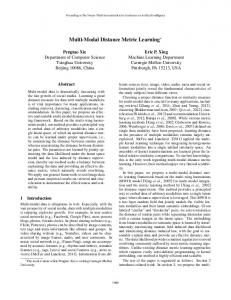
In the popular classification task, many approaches in the last decade have exploited the same classification framework [Lazebnik et al., 2006, Yang et al., 2009, Liu et al., 2011], the only difference between them is how they fine-tuned the low-level and mid-level feature extraction process to gain in recognition performance. To better understand this rush for performance, we describe the popular visual Bag-of-Words image representation model that is illustrated in Fig. 1.1 and inspired from the Bag-of-Words used in text information retrieval. The text Bag-of-Words model represents a document by a histogram, it assigns to each term in a document a weight for that term that depends on the number of occurrences of the term 9 http://www.image-net.org/challenges/LSVRC/2012/
5
Chapter 1. Background
Input images:
Image representations:
Codebook of visual words:
Figure 1.1: An illustration of the visual Bag-of-Words (BoW) representation for three input images: the presence of visual words from a codebook (bottom row) in input images (top row) is quantified in a histogram. The histogram of “word counts” (middle row) is used to represent the image. Image courtesy of Li Fei-Fei. in the document. In the visual BoW model, images are first decomposed as a set of local features, usually obtained by regular grid-based sampling (i.e., images are segmented as patches that are regularly spaced). Converting the set of local descriptors of an image into the final image representation is performed by a succession of two steps: coding and pooling. In the original BoW model, coding consists in assigning each local descriptor to the closest visual word, while pooling averages the local descriptor projections. The final BoW vector, which is the representation of the image, can thus be regarded as a histogram counting the occurrences of each visual word in the image. Since the notion of “word” is not as easily interpretable for image classification as for text retrieval, many efforts have been devoted to improve coding and pooling. Fig. 1.2 illustrates the whole classification pipeline of the visual Bag-of-Words model for image classification. Local features are first extracted from the input image, and encoded into an off-line trained dictionary. The codes are then pooled to generate the image signature. This mid-level representation is subsequently normalized before training the classifier, which is usually a Support Vector Machine (SVM) [Cortes and Vapnik, 1995] model. Each block of the figure is detailed in the following. A pioneer work using the visual BoW framework is probably Netra [Ma and Manjunath, 1997] which exploits color feature dictionary learning. 1.1.1.1
Low-level feature extraction
The first step of the BoW framework corresponds to local feature extraction. To extract local descriptors, one first issue is to detect relevant image regions. Many attempts have been done to achieve that goal, generally based on a geometric criterion, using Harris affine region detector [Harris and Stephens, 1988] or its multi-scale version [Mikolajczyk and Schmid, 2004], SIFT detector [Lowe, 2004], etc. However, for classification tasks, most evaluations reveal that a regular grid-based sampling strategy leads to optimal performances [Fei-Fei and Perona, 2005]. In each region of the image, SIFT descriptors [Lowe, 2004] are computed because of their excellent performances attested in various datasets. 1.1.1.2
Mid-level coding and pooling scheme
We explain here how to compute the mid-level representation of images in order to obtain their BoW representations. 6
1.1. Image Representations for Classification
Low level Feature Extraction Feature Extraction
Image
Mid level Representation
Local Features
Feature Coding
Pooling
Visual Codes
Normalization and Learning
Normalization
Vector Image Representation
Normalized Signature
SVM Classifier
Category Label
Figure 1.2: BoW pipeline for classification Let X = (x1 , . . . , xj , . . . , xN ) be the set of local descriptors in an image, where N is the number of local descriptors in the image. In the BoW model, the mid-level signature generation first requires a set � M of visual words (also called codewords) bi ∈ Rd i=1 (where d is the local descriptor’s dimensionality, and M is the number of visual words). This set of visual words is called visual codebook or dictionary, we denote it B. Table 1.1 gives a matrix illustration of the mid-level representation extraction in the BoW pipeline, for scalar coding and pooling schemes. The set of local descriptors X is represented in columns, while the set of dictionary elements B occupies the rows. One column of the matrix thus represents the encoding of a given local descriptor xj into the codebook, that we denote as f (xj ) = uj = (u1,j , u2,j , · · · , uM,j ) ∈ RM . In each row, aggregating the codes for a given dictionary element bi results in the pooling operation, denoted as g(X, f ). Codebook Different strategies to compute the codebook exist. The codebook can be determined with a static clustering, e.g., Smith and Chang [Smith and Chang, 1997] use a codebook of 166 regular colors defined a priori. These techniques are generally far from optimal, except in very specific applications. Usually, the codebook is learned using an unsupervised clustering algorithm applied on local descriptors randomly selected from an image dataset, providing a set of M clusters with centers bi . K-means is widely used in the BoW pipeline. Other approaches [Boureau et al., 2010, Goh et al., 2012] try to include supervision to improve the dictionary learning. However, Coates and Ng [Coates and Ng, 2011] report that dictionary elements learned with “naive” unsupervised methods (e.g., k-means or even random sampling) are sufficient to reach high performances on different image datasets. They also claim [Coates and Ng, 2011] that the recognition performance mostly depends on the choice of architecture. Specifically a good encoding function (i.e., sparse or soft) is required. Coding The coding step has attracted a lot of attention in the computer vision community, different coding methods have thus been proposed. In the original BoW model, the value of ui,j is 1 if bi is the nearest visual word of xj and 0 otherwise. This method is called hard assignment or hard coding. In other methods, such as the Local Soft Coding (LSC) algorithm [Liu et al., 2011], the value of ui,j is between 0 and 1 and grows with the relative proximity between xj and the codeword bi . Note that some representation models, such as Fisher vector [Perronnin and Dance, 2007] or VLAD [J´egou et al., 2010] descriptors, use a vector representation of ui,j ∈ RP , which results in vectors uj in RP M . For instance, the Fisher Vector model [Perronnin et al., 2010] extends the BoW by encoding the average first- and second-order differences between the descriptors and codewords. Pooling The pooling step aggregates the resulting codes ui,j in order to compute the final vector image representation z = {zi }ni=1 of the image. The two most popular pooling methods are the sum and the max PNpoolings. Sum pooling counts the number of occurences of each codeword in the image (i.e., zi = j=1 ui,j ). Max pooling detects for each codeword its maximum score among all the patches of the image (i.e., zi = maxj∈{1,...,N } ui,j ). Sum pooling is particularly useful when hard coding is applied since max pooling would return binary values of zi in this context. In the context of soft coding, where codes are usually real values between 0 and 1, the max pooling plays the role of a codeword detector. Other 7
Chapter 1. Background
b1
x1 u1,1 .. .
···
bi
ui,1 .. .
···
bM
uM,1
···
xj u1,j .. .
···
xN u1,N .. .
···
ui,N .. .
uM,j · · · ⇓ f : coding
uM,N
ui,j .. .
⇒ g : pooling
Table 1.1: Coding and pooling strategies. The functions f and g are explicited below
pooling methods have been proposed. For instance, the BossaNova representation [Avila et al., 2013] keeps more information than the BoW during the pooling step by estimating the distribution of the descriptors around each codeword. 1.1.1.3
Normalization and learning
Once the signatures of the different images in the dataset are computed, the classic approach is to learn a statistical machine learning model, usually an SVM learned using a one-against-all strategy. Some authors normalize the image representations before learning the classifers [Perronnin et al., 2010, Avila et al., 2013]. The choice of normalization also depends on the chosen representation model and classifier model (e.g., linear or non-linear SVM). 1.1.1.4
Beyond Bag-of-Words
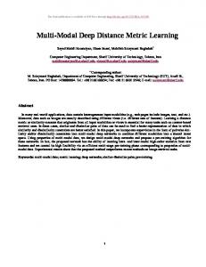
The pipeline described in Fig. 1.2 has been exploited in the last decade by many approaches on various datasets [Lazebnik et al., 2006, Yang et al., 2009, Perronnin et al., 2010, Liu et al., 2011]. In particular, many attempts for improving the coding and pooling steps have been done. Fig. 1.3 illustrates the performance evaluations of different state-of-the-art methods on the Caltech-101 [Fei-Fei et al., 2007] dataset. Most of them are extensions of the Bag-of-Words model which improve its mid-level representation. The improvement of the mid-level step since 2006 significantly boosted performances: for example, using 30 training examples, there is a substantial gain of about 20 points from the baseline work of Lazebnik et al. [Lazebnik et al., 2006] (∼ 64% in 2006) to the pooling learning method of Feng et al. [Feng et al., 2011] (∼ 83% in 2011). This work on the BoW model over years demonstrates in this particular application task that the performance of machine learning methods is heavily dependent on the choice of data representations. Especially, as a preliminary of this thesis, we performed a thorough study of the different low-level and mid-level parameters of this pipeline that have an impact on classification performance. This study led to the following publications [Law et al., 2012a, Law et al., 2014a]. While the methods mentioned above are interested in manually tuning the extraction process to generate a useful image representation, other methods are concerned with questions surrounding how we can best learn meaningful and useful representations of data. The latter approach is known as representation learning and includes distance metric learning.
1.1.2
Deep representations
In the last decade, datasets of labeled images for computer vision tasks (e.g., image classification or detection) have grown considerably. Recently, the handcrafted extensions of the BoW pipeline have been substantially outperformed by the latest generation of Convolutional Neural Networks (CNNs) 8
1.1. Image Representations for Classification
85
� ♣ H ~ � F N
80
♣ H � N
70
• �
• Accuracy (%)
60
� •
50
• �
♥
♥
• ♥ 40
♥
� ♣ H ~ �
30
20
♠ 10
♥
♥
5 10 15 20 25 Number of training images per category
F N • � ♥ ♠
[Feng et al., 2011] (CVPR) [Duchenne et al., 2011] (ICCV) [Goh et al., 2012] (ECCV) [Perronnin et al., 2010] (ECCV) reimplemented by [Chatfield et al., 2011] [Wang et al., 2010] (CVPR) reimplemented by [Chatfield et al., 2011] [Liu et al., 2011] (ICCV) [Yang et al., 2009] (CVPR) [Zhang et al., 2006] (CVPR) [Lazebnik et al., 2006] (CVPR) [Grauman and Darrell, 2005] (ICCV) SSD baseline 30
Figure 1.3: State-of-the-art results since 2006 on the Caltech 101 dataset for BoW pipeline methods in mono-feature setup.
[LeCun et al., 1989] to many tasks that involve very large datasets, particularly in classification and detection [Krizhevsky et al., 2012, Szegedy et al., 2013]. The general idea of deep representations is to learn a hierarchy of representations from a dataset of images. CNNs have a substantially more sophisticated structure than standard (shallow) representations such as BoWs. They comprise several layers of nonlinear feature extractors, and are therefore said to be deep. The representation at each level is composed of lower-level ones. Since they involve a very large number of parameters to learn, they benefit from large scale datasets of images to limit overfitting10 . Note that an architecture with at least four layers is considered to be a deep representation [Hinton et al., 2006, Bengio et al., 2007]. The architecture of CNNs takes raw input data at the lowest level (i.e., pixels) and processes them via a sequence of basic computational units until the data is transformed to a suitable representation in the higher layers to perform classification. Deep connectionist models learn a mapping from input data to output classes by attempting to untangle the manifold of the highly nonlinear input space [LeCun et al., 1989]. The strength of these models is that they are learned entirely in a supervised way from the pixel level to the class level. Furthermore, recent work observed the relevance of deep models for transfer learning. Features learned on the ImageNet dataset may be used successfully in action recognition on a different benchmark dataset 10 CNNs also benefit from other improvements, such as GPU computation and data augmentation (also known as virtual sampling or data jittering).
9
Chapter 1. Background [Oquab et al., 2014]. Recently, the enthusiasm of computer vision researchers for CNNs has reached the same level as the enthusiasm they had for BoWs some years ago. Many recent works try to extend CNNs to increase performance in the same way as they extended BoW. For instance, at the ImageNet LargeScale Visual Recognition Challenge (ILSVRC) 201411 , the first and second places in the localisation and classification tracks respectively, were achieved by a very deep architecture that has more than 15 weight layers [Simonyan and Zisserman, 2014]. By contrast, the winner of the ILSVRC-2012 challenge had 8 layers. The interested reader on deep learning of representations can refer to [Bengio, 2013]. Conclusion The choice of an appropriate image representation model remains a challenging task for the good performance of recognition methods in many computer vision contexts. For instance, deep learning which learns how to represent images directly from pixels, obtains state-of-the results in the context of image classification when the model is trained on very large datasets. From this observation, learning representations seems a promising paradigm to investigate for computer vision tasks such as image classification. In this thesis, we focus on a special case of representation learning which consists in learning an appropriate distance metric to compare images. For instance, we want to be able to determine whether two images represent the same object or not. For this purpose, we take some given image representation (e.g., BoW or deep features) as input of our model and infer a metric whose goal is to compare two (possibly never seen) images. Our task actually learns a new transformation of the input data such that the Euclidean distance in the transformed space satisfies most of the desired properties. We present in the next section some interesting representation learning contexts where an appropriate metric is learned.
1.2
Metric Learning for Computer Vision
Metrics play an important role for comparing images in many machine learning and computer vision problems. In this section, we briefly present contexts where learning an appropriate metric may be useful. Some successful examples of applications that greatly depend on the choice of metric are: k-Nearest Neighbors (k-NN) classification [Cover and Hart, 1967] where an object is classified by a majority vote of its nearest neighbors: the object is assigned to the class most common among its k nearest neighbors. The nearest neighbors are determined based on a given metric (usually the Euclidean distance in the input space). Notably, a recent work [Mensink et al., 2013] has shown that a metric learned for k-NN reaches state-of-the-art performance when new images or classes are integrated in the dataset. KMeans clustering [Steinhaus, 1956, MacQueen et al., 1967] aims at partitioning the training set into K clusters in which each sample belongs to the cluster with the nearest mean. Test samples are assigned to the nearest cluster by distance. Information/Image retrieval [Salton, 1975, Goodrum, 2000] returns (the most) similar samples to a given query. Kernel methods [Scholkopf and Smola, 2001] exploit kernel functions, a special case of similarity metrics. The most popular example of kernel methods is the Support Vector Machines (SVM) model [Cortes and Vapnik, 1995] for which the choice of the kernel, which is critical to the success of the method, is typically left to the user. Moreover, when the data is multimodal (i.e., heterogeneous), multiple kernel learning (MKL) methods [Bach et al., 2004, Rakotomamonjy et al., 2008] allow to integrate data into a single, unified space and compare them. Contexts that transform the input data into another space (usually with lower dimensionality) to make it interpretable are considered as metric learning approaches. Some examples are: Manifold learning Humans often have difficulty comprehending data in many dimensions (more than 3). Thus, reducing data to a small number of dimensions is useful for visualization purposes. Moreover, reducing data into fewer dimensions often makes analysis algorithms more efficient, and can help machine learning algorithms make more accurate predictions. One approach to simplification is to assume that 11 http://www.image-net.org/challenges/LSVRC/2014/
10
1.2. Metric Learning for Computer Vision Polar bear: is black: is white: is brown: has stripes: eats fish:
no yes no no yes
Otter: is black: is white: is brown: has stripes: eats fish:
yes no yes no yes
Zebra: is black: is white: is brown: has stripes: eats fish:
yes yes no yes no
Figure 1.4: High-level attributes describe categories of objects (here animals) with information that is understandable by humans. Images from the Animals with Attributes dataset [Lampert et al., 2009].
the data of interest lies on an embedded non-linear manifold within the higher-dimensional space. If the manifold is of low enough dimensionality, the data can be visualised in the low-dimensional space. The key idea of manifold learning is to learn an underlying low-dimensional manifold preserving the distances between observed data points. Some good representatives of manifold learning are Multidimensional Scaling (MDS) [Borg and Groenen, 2005] and Isomap [Tenenbaum et al., 2000]. Since manifold learning methods do not consider labels of data to learn the low-dimensional space, they are considered as unsupervised metric learning approaches.
Eigenvector methods Eigenvector methods such as Linear Discriminant Analysis (LDA) [Fisher, 1938] or Principal Component Analysis (PCA) [Galton, 1889, Pearson, 1901, Hotelling, 1933] have been widely used to discover informative linear transformations of the input space. They learn a linear transformation x 7−→ Lx that projects the training inputs in another space that satisfies some criterion. For instance, PCA projects training inputs into a variance-maximizing subspace while LDA maximizes the amount of between-class variance relative to the amount of within-class variance. PCA can be viewed as a simple linear form of linear manifold learning, i.e., characterizing a lower-dimensional region in input space near which the data density is peaked [Bengio et al., 2013].
Visual high-level attributes While traditional visual recognition approaches map low-level image features directly to object category labels, some recent works have proposed to focus on visual attributes [Farhadi et al., 2009, Lampert et al., 2009]. Visual attributes are high-level descriptions of concepts in images. Generally, they have human-designated names (e.g., striped, four-legged, see Fig. 1.4) and are valuable tools to give a semantic meaning to objects or classes in various problems. They are also easy to interpret and manipulate. Visual attributes have shown their benefit in face verification [Kumar et al., 2009] and object classification [Lampert et al., 2009, Akata et al., 2013], particularly in the context of zero-shot learning for which the goal is to learn a classifier that must predict novel categories that were omitted from the training set. It is particularly useful for contexts where datasets are large and dynamic (i.e., new images and new classes can be added and the semantics of existing classes might evolve). Indeed, when images of new labels are introduced in the dataset, discriminative models, such as SVM, have to be relearned at a relatively high computational cost in large scale settings (i.e., when the dataset contains more than 10 million images and 10,000 categories). Methods that learn 11
Chapter 1. Background Attribute: is natural
≺ class (d)
Attribute: smiles
≺ class (e)
∼ class (f )
class (g)
class (h)
Figure 1.5: Relative attributes: high-level descriptions of classes are given as a function of other classes. While it is difficult to determine whether the image of class (e) is natural or not, it is easier to say that it is more natural than class (d) and less natural than class (f ). Scarlett Johansson (class (g)) smiles as much as Miley Cyrus (class (h)). an appropriate metric [Akata et al., 2013, Mensink et al., 2013] have shown promising results in these contexts since the learned metric can be generalized to new images. In many attribute problems [Parikh and Grauman, 2011, Yu et al., 2013, Akata et al., 2013], a (linear) transformation is learned so that low-level representations of images are projected into a high-level semantic space. Such a space is usually constructed so that each dimension describes the degree of presence of an attribute in a given image. In other words, an image is described by a vector, and each element of the vector is the degree of presence of a given attribute in the image. In the high-level space, images can be semantically compared to one another. One of the most popular contexts that compare images with attributes is the relative attribute problem [Parikh and Grauman, 2011]. In this problem, the representations of images in the high-level semantic space are learned relatively to the learned representations of other images. The original relative attribute problem considers relations between pairs of classes: • inequality constraints: i.e., (e) ≺ (f ): the presence of an attribute is stronger in class (f ) than in class (e) • and equivalence constraints: i.e., (g) ∼ (h): the presence of an attribute is equivalent in class (g) and class (h). This type of relationship is particularly useful when a boolean score for the presence an attribute is difficult to annotate for a class or an image (see Fig. 1.5). Relative attributes have also been used in image retrieval [Kovashka et al., 2012] to find objects that match semantic queries (e.g., an example query would be “Find a red shoe that is shinier than some given image of shoe”). Conclusion Similarity metrics are key ingredients of many applications, such as image retrieval. The choice of metric is a difficult task and is determined by the problem at hand. An appropriate metric can be picked by experts in some problems, but it can also be learned to improve performance. In this dissertation, we are interested in supervised distance metric learning that we present in the following.
12
1.3. Supervised Distance Metric Learning
1.3 1.3.1
Supervised Distance Metric Learning Notations
Throughout this thesis, Sd , Sd+ and Sd++ denote the sets of d×d real-valued symmetric, symmetric positive semidefinite (PSD) matrices and symmetric positive definite matrices, respectively. The set of considered images is P = {Ii }Ii=1 , each image Ii is represented by a feature vector xi ∈ Rd . For matrices A ∈ Rb×c and B ∈ Rb×c , denote the Frobenius inner product by hA, Bi = tr(A> B) where tr denotes the trace of a matrix. ΠC (x) is the Euclidean projection of the vector or matrix x on the convex set C (see Chapter 8.1 in [Boyd and Vandenberghe, 2004]). For a given vector a = (a1 , . . . , ad )> ∈ Rd , Diag(a) = A ∈ Sd corresponds to a square diagonal matrix such that ∀i, Aii = ai where A = [Aij ]. For a given square matrix A ∈ Rd×d , Diag(A) = a ∈ Rd corresponds to the diagonal elements of A set in a vector: i.e., ai = Aii . λ(A) is the vector of eigenvalues of matrix A arranged in non-increasing order. λ(A)i is the i-th largest eigenvalue of A. Finally, for x ∈ R, let [x]+ = max(0, x).
1.3.2
Distance and similarity metrics
The choice of an appropriate metric is crucial in many machine learning and computer vision problems For some problems, the selected metric and its parameters are fine-tuned by experts, but its choice remains a difficult task in general. Extensive work has been done to learn relevant metrics from labeled or unlabeled data. The most useful property of metrics in this thesis is that they can be used to compare two never seen samples, i.e., that were not present in the training dataset. We present here widely used metrics in computer vision, especially the Mahalanobis distance metric which is the focus of this thesis. Minkowski distances The Minkowski distance is a metric on Euclidean space which can be considered as a generalization of both the Euclidean distance and the Manhattan distance. The Minkowski distance of order p ≥ 1 between two points x = (x1 , x2 , . . . , xd ) ∈ Rd and z = (z1 , z2 , . . . , zd ) ∈ Rd is defined as: d X
!1/p |xi − zi |p
= kx − zkp
i=1
The most wildy used Minkowski distance in Computer Vision is the Euclidean distance, which corresponds to p = 2. Note that for p < 1, the triangle inequality is violated. Histogram distances In some contexts, the data is sampled from a probability simplex defined as Pd = {x ∈ Rd |x ≥ 0, x> 1 = 1} where 1 ∈ Rd denotes the vector of all-ones. Each input x ∈ Pd can be interpreted as a histogram over d buckets. Examples of applications that use this type of data are ubiquitous in computer vision (e.g., distributions over visual codebooks [Tuytelaars and Mikolajczyk, 2008] or histograms of colors [Stricker and Orengo, 1995]). Different distance metrics have been proposed to compare such histograms: e.g., quadratic-form distance [Globerson and Roweis, 2007], Earth Mover’s distance [Rubner et al., 2000]. One of the most popular distance metrics is the χ2 histogram distance whose origin is the χ2 statistical hypothesis test [Mood, 1950]. It is formulated as: d
Dχ2 (x, z) =
1 X (xi − zi )2 2 i=1 xi + zi
and has been successfully applied in many computer vision domains. Some successful examples are [Cula and Dana, 2004, Tuytelaars and Mikolajczyk, 2008, Varma and Zisserman, 2009]. 13
Chapter 1. Background Mahalanobis(-like) distance metric We present here Mahalanobis distance metrics that are the focus of this thesis and the most popular type of learned distance metrics in the machine learning and computer vision communities. The Mahalanobis distance [Mahalanobis, 1936] is originally a measure of the distance between an observation x and from a group of observations with mean µ and covariance matrix Σ: 2 > −1 (x − µ) DΣ −1 (x) = (x − µ) Σ
(1.1)
It can also be defined as a dissimilarity measure between two random vectors x and x0 of the same distribution with the covariance matrix Σ: 2 0 0 > −1 DΣ (x − x0 ) −1 (x, x ) = (x − x ) Σ
In this thesis, we consider that a Mahalanobis distance metric is any dissimilarity function parameterized by a symmetric positive semidefinite (PSD) matrix M. It is written in this form: 2 DM (Ii , Ij ) = (xi − xj )> M(xi − xj ) = hM, (xi − xj )(xi − xj )> i s.t. M ∈ Sd+ 2 where Sd+ is the set of symmetric positive semidefinite matrices. This formulation guarantees that DM is a pseudo-metric (i.e., it is symmetric, its value is nonnegative and it satisfies the triangle inequality). In this thesis, we will often refer to pseudo-metrics as metrics to simplify the discussion.
The mere fact that the learned model has to be in Sd+ , which is a proper cone (see Definition A.1.3), makes the learning framework more complex than classic optimization problems for which the domain (i.e., search space) is the whole input space. We give the definition of positive semidefiniteness for matrices: Definition 1.3.1. (Positive semidefinite matrix) A matrix A ∈ Rd×d is positive semidefinite (PSD) iff it satisfies: ∀x ∈ Rd , x> Ax ≥ 0 PSD matrices can be nonsymmetric (see [Dattorro, 2005], Appendix A). However, we are only interested in symmetric PSD matrices in this thesis. When we define a PSD matrix, we implicitly consider that it is symmetric. The set Sd+ is fundamental in Mahalanobis distance metric learning approaches, the interested reader can refer to Appendix A for details on Sd+ and its properties. The main property to know is that a matrix M is in Sd+ iff it can be rewritten as M = L> L where L ∈ Re×d and e ≥ rank(M). From this property, the (squared) Mahalanobis distance metric DM can be rewritten equivalently: 2 DM (Ii , Ij ) = (xi − xj )> M(xi − xj )
= (xi − xj )> L> L(xi − xj ) = kL(xi − xj )k22 = kLxi − Lxj k22 A Mahalanobis distance metric parameterized by the matrix M = L> L can then be seen as calculating the Euclidean distance in the space induced by the linear transformation parameterized by L. Actually, since Mahalanobis distance metrics can be induced from linear transformations and vice versa, any method that returns a linear transformation can be considered as a metric learning method. For this reason, methods such as Principal component analysis (PCA) and Linear discriminant analysis (LDA) can be seen as metric learning approaches. Some approaches [Shalev-Shwartz et al., 2004, Globerson and Roweis, 2006, Mignon and Jurie, 2012] have extended Mahalanobis distance metric so that a non-linear mapping is learned. Instead of considering the linear transformation x 7−→ Lx, they consider the transformation x 7−→ L(φ(x)) where φ is a mapping 14
1.3. Supervised Distance Metric Learning from the input space (denoted X ) to a reproducing kernel Hilbert space (RKHS) H. The data is then mapped to RN by a linear transformation L : H −→ RN . Since φ can be non-linear, this allows to learn 2 a non-linear metric DM (Ii , Ij ) = kL(φ(xi )) − L(φ(xj ))k22 . By exploiting the generalized representer theorem [Sch¨olkopf et al., 2001], the operator L can be expressed as the matrix product L = PΦ> where Φ is a matrix representation of X in H (i.e., the i-th column of Φ is φ(xi ) for i = {1, · · · , N }) and for some real-valued matrix P ∈ Re×N (with the parameter e > 0 manually chosen). By denoting K ∈ SN + the kernel matrix: K = Φ> Φ = [Kij ] with Kij = hφ(xi ), φ(xj )i = k(xi , xj ) the non-linear mapping can be written: N
L(φ(x)) = PΦ> (φ(x)) = P(hφ(xi ), φ(x))i)N i=1 = P (k(xi , x))i=1 where (·)N p=1 denotes concatenation in a N -dimensional vector. The main limitation of this approach is that the resulting computational complexity, which depends on the size of the dataset, is generally increased for a relatively small gain in recognition performance. Since the number of independent parameters can be very large when N is large, the risk of overfitting is high. For computational reasons and to avoid overfitting, a simple linear mapping is generally used for Mahalanobis distance metrics. Bilinear Similarity An approach very similar to Mahalanobis distance metric is the bilinear similarity. The bilinear similarity between two vectors x ∈ Rd and z ∈ Re is formulated as: SM (x, z) = x> Mz where the matrix M ∈ Rd×e is not required to be PSD nor square. When d = e and M is in Sd+ , this corresponds to the similarity function SM (x, z) = hLx, Lzi where M = L> L. This type of similarity has been used for image classification [Chechik et al., 2009] and retrieval [Chechik et al., 2009, Deng et al., 2011]. It has two main advantages: when the vectors x and z are sparse and have kx and kz nonzero elements, SM (x, z) can be computed in O(kx kz ) time. Moreover, it can be used to compare objects of different types: for instance, in [Akata et al., 2013], images and attributes (high-level descriptions of concepts) are embedded and compared in a single space.
1.3.3
Learning scheme
The goal of supervised distance metric learning is to infer a (linear) transformation that is optimized for a specific prediction task, such as ranking or nearest-neighbor classification. The transformation induces a distance metric that is generally learned so that distances between similar (resp. dissimilar) samples are small (resp. large) or to preserve orders of distances between training samples. Metric Learning has been applied to compare different types of data representations such as vectors, character strings or trees (see [Bellet et al., 2013] for details). In this thesis, we focus on learning distance metrics to compare vector representations of images (or webpages). Distance metric learning is an area of machine learning and, as such, the formulation of its problems is similar to many (supervised) machine learning problems. In this section, we present the general formulation of machine learning problems, and particularly focus on metric learning problems. 1.3.3.1
Optimization problem
A metric learning algorithm aims at determining the matrix M ∈ Rd×d such that the metric parameterized by M satisfies most of the constraints defined by the training information. The training information is usually either: 15
Chapter 1. Background • Similar/Dissimilar pairs: the training set is composed of a set S of similar pairs of samples, and a set D of dissimilar pairs of samples. • Ordered relations of distances: the training set is composed of a set T = {(Ii , Ii+ , Ii− )}i of triplets of samples. The goal is to learn a distance metric such that the distance between Ii and Ii+ is smaller than the distance between Ii and Ii− . The way the training information is provided and exploited will be discussed in Section 1.4. For simplicity, we consider that all the sets S, D and T are subsets of the training set N . Metric learning problems are generally formulated as an optimization problem of the form: min µR(M) + `(M, N ) s.t. M ∈ C M
(1.2)
where C an arbitrary convex domain (e.g., Sd or Sd+ ), `(M, N ) is a loss function that penalizes constraints that are not satisfied by the model induced by M, R(M) is a regularization term on the parameter M, and µ ≥ 0 is the regularization parameter. The loss function `(M, N ) measures the ability of the matrix M to satisfy some distance constraints provided by the training set N . The details on the design of the set N and the loss `(M, N ) are specified in the following. In this thesis, we only consider the case where the learned model is a Mahalanobis(-like) distance 2 (Ii , Ij ) = (xi − xj )> M(xi − xj )). metric (i.e., C = Sd+ , and the model is the metric DM 1.3.3.2
Loss and surrogate functions
Choosing an appropriate loss function is not an easy task and strongly depends on the problem at hand. In order to explain surrogate functions, we first need to introduce how training data is provided and exploited in supervised machine learning problems. We use the binary-class classification setting as a reference problem for explanation. We are given a set of n training samples {(x1 , y1 ), (x2 , y2 ), · · · , (xn , yn )} where each xi belongs to some input space X , usually Rd , and yi ∈ {−1, 1} is the class label of xi . The goal of classification machine learning algorithms is to find a model that maximizes the number of correct labels predicted for a given set of test samples. For this purpose, we are given a loss function L : {−1, 1} × {−1, 1} −→ R that measures the error of a given prediction. The loss function L takes as argument an arbitrary point (ˆ y , y), and its value is interpreted as the cost incurred by predicting the label yˆ when the true label is y. In the classification context, this loss function L is usually the zero-one (0/1) loss, i.e., L(ˆ y , y) = 0 if y = yˆ, and L(ˆ y , y) = 1 otherwise. The goal is then to find a classifier, represented by the function h : X −→ {−1, 1}, with the smallest expected loss on a new sample. However, the probability distribution of the variables is usually unknown to the learning algorithm, and computing the exact expected value is not possible. That is why it is approximated by averaging the loss function on the training set (i.e., averaging the number of wrongly classified examples in the training set): n
1X Remp (h) = L(h(xi ), yi ) n i=1 which is called the empirical risk. Empirical risk minimization states that the learning algorithm should ˆ which minimizes the empirical risk h ˆ = argmin choose a hypothesis h h∈F Remp (h) where F is a fixed class of functions. ˆ that maximizes the number of correctly Another issue is that the problem of finding the function h classified training examples is NP-hard. The 0/1 loss is therefore generally replaced by a proxy to the loss, called a surrogate loss function, which is usually convex and hence has better convergence properties. The interested reader can refer to [Bartlett et al., 2006, Tewari and Bartlett, 2007]. For classification, the most commonly used surrogate loss functions (with y ∈ {−1, 1} and h(x) ∈ R) are: 16
1.3. Supervised Distance Metric Learning
Classification error (0/1 loss) Hinge loss Modified Huber loss Exponential loss Logistic loss Squared hinge loss
5
L(h(x), y)
4
3
2
1
0 −3
−2
−1
0
1
2
3
yh(x) Figure 1.6: Examples of surrogate loss functions for the zero-one loss. • the hinge loss `hinge (h(x), y) = [1 − yh(x)]+ = max (0, 1 − yh(x)) used in the support vector machine (SVM) [Cortes and Vapnik, 1995] (note that slack variables used in SVMs are equivalent to the hinge loss function: the non-negative ξ that minimizes the constraint t ≥ 1−ξ is max(0, 1−t)). 2
• the squared hinge loss `2hinge (h(x), y) = [1 − yh(x)]2+ = max (0, 1 − yh(x)) used for relative attributes [Parikh and Grauman, 2011]. • The modified Huber loss [Chapelle, 2007], a differentiable approximation of the hinge loss: Lγhub (h(x), y)
=
0
(1+γ−yh(x))2 4γ
1 − yh(x)
if if if
yh(x) > 1 + γ |1 − yh(x)| ≤ γ yh(x) < 1 − γ
(zero loss) (quadratic part) (linear part)
where γ is typically a value in [0.01, 0.5]. • the exponential loss: `exp (h(x), y) = e−yh(x) used in Adaboost [Freund and Schapire, 1995]. • the logistic loss: `βlog (h(x), y) = β1 ln(1 + e−yβh(x) ) used in Logitboost [Friedman et al., 2000] and PCCA [Mignon and Jurie, 2012]. Fig. 1.6 illustrates these loss functions12 along with the nonconvex 0/1 loss. Since multiple surrogate loss functions exist to replace the 0/1 loss, a natural question is “which one should be chosen?”. The answer strongly depends on the application task and the training data. In the context of classification, Rosasco et al. [Rosasco et al., 2004] concluded that the hinge loss has better convergence rate than the logistic loss. Chapelle [Chapelle, 2007] proposed to use the squared hinge loss or the modified Huber loss functions that have better convergence rate than the hinge loss by using Newton’s method. The interested reader can refer to [Mahdavi, 2014].
1.3.4
Review of popular metric learning approaches
We present some of the most popular approaches in metric learning. We particularly focus on Mahalanobis distance metric learning where the goal is to learn a distance metric parameterized by a matrix M ∈ Sd+ 2 such that the learned metric can be formulated: DM (Ii , Ij ) = Φ(Ii , Ij )> MΦ(Ii , Ij ) = hM, Cij i where > Cij = Φ(Ii , Ij )Φ(Ii , Ij ) and Φ(Ii , Ij ) is usually (xi − xj ). For an exhaustive list of metric learning algorithms, the interested reader can read the recent surveys of [Kulis, 2012, Bellet et al., 2013]. 12 For
the logistic loss, we actually plot `log2 (h(x), y) = log(1 + e−yh(x) ) − log(2) + 1.
17
Chapter 1. Background 1.3.4.1
MMC (Xing et al.)
The work of [Xing et al., 2002] is the first Mahalanobis distance metric learning problem. It relies on a convex Semi-Definite Programming (SDP) formulation which aims at minimizing the distances of similar samples while maintaining the sum of the dissimilar samples beyond a given threshold (here 1)13 : X
min
M∈Sd +
2 DM (Ii , Ij ) s.t.
(Ii ,Ij )∈S
X
q
2 (I , I ) ≥ 1 DM i j
(1.3)
(Ii ,Ij )∈D
P 2 The term (Ii ,Ij )∈S DM (Ii , Ij ) can be seen as a regularization term [Kulis, 2012] as will be explained in Section 1.5.1. The main drawback of the method is the basic SDP solver proposed by [Xing et al., 2002] which makes it unscalable. Moreover, there is no regularization term to control the rank of the solution, this can lead to high-rank solutions that are prone to overfitting.
1.3.4.2
Schultz & Joachims’ method
Schultz and Joachims [Schultz and Joachims, 2004] propose to write the PSD matrix M = AWA where A is a fixed matrix, and the matrix W is diagonal. Instead of working on similar/dissimilar pairs as 2 in [Xing et al., 2002], they work on triplets (Ii , Ii+ , Ii− ) ∈ T and want the distance DM (Ii , Ii+ ) to be − 2 smaller than DM (Ii , Ii ). For this purpose, they write their problem as: X
min kMk2F +
M∈Sd +
ξi
(Ii ,Ii+ ,Ii− )∈T
2 2 s.t. ∀(Ii , Ii+ , Ii− ) ∈ T , DM (Ii , Ii− ) ≥ 1 + DM (Ii , Ii+ ) − ξi
(1.4)
ξi ≥ 0, M = AWA, A fixed, W diagonal where kMk2F is the squared Frobenius norm of M. Slack variables ξi are introduced to allow penalized constraints. The problem in Eq. (1.4) is convex and actually an extension of RankSVM [Joachims, 2002], it can thus be solved efficiently. The main drawback of the method is that the learned matrix W is diagonal, which limits the domain of the solution but greatly reduces the number of learned parameters to d) and thus limits overfitting. Moreover, the matrix A has to be chosen carefully. (from d(d+1) 2 1.3.4.3
Neighbourhood Component Analysis (NCA)
Neighbourhood Component Analysis (NCA) [Goldberger et al., 2004] is the first approach that learns a Mahalanobis distance metric for k-NN classification. They consider the multi-class classification problem and want to find a distance metric that maximizes the performance of nearest neighbor classification. Ideally, they would like to optimize performance on future test data, but since they do not know the true data distribution, they instead attempt to optimize leave-one-out (LOO) performance on the training data. For this purpose, they consider the decomposition M = L> L. They introduce a differentiable cost function based on stochastic neighbor assignments in the space induced by L. Each point Ii selects another point Ij as its neighbor with some probability pij , and inherits its class label from the point it selects. They define the pij using a softmax over Euclidean distances in the space induced by L: 2 exp(−DM (Ii , Ij )) exp(−kLxi − Lxj k22 ) P = 2 2 k6=i exp(−kLxi − Lxk k2 ) k6=i exp(−DM (Ii , Ik ))
pij = P 13 The
authors use the constraint learning a matrix M that is rank 1.
18
P
(Ii ,Ij )∈D
pii = 0
q 2 (I , I ) instead of the usual squared Mahalanobis distance to avoid DM i j
1.3. Supervised Distance Metric Learning
Figure 1.7: LMNN: schematic illustration of one input’s neighborhood before training (left) versus after training (right). The learned distance metric is optimized so that the k = 3 target neighbors of the input image are its nearest neighbors. Image courtesy of Kilian Weinberger [Weinberger and Saul, 2009].
Let yi be the class label of Ii , and denote Ci = {Ij | yi = yj } the set of images in the same class as Ii . Their objective problem then tries to maximize: XX max pij L
i
j∈Ci
This problem is nonconvex and the optimization scheme is thus subject to local maxima.
1.3.4.4
Large Margin Nearest Neighbors (LMNN)
LMNN [Weinberger et al., 2005, Weinberger and Saul, 2009] is the most popular nearest neighbor metric learning algorithm. For each sample Ii , LMNN tries to satisfy the condition that members of a predefined set of k target neighbors (of the same class yi ) are closer than samples from other classes. In [Weinberger and Saul, 2009], those target neighbors are chosen using the `2 -distance in the input space. Formally, the constraints are defined in the following way: S ={(Ii , Ij ) | yi = yj and Ij is one of the k target neighbors of Ii } T ={(Ii , Ij , Ik ) | (Ii , Ij ) ∈ S, yi = yj 6= yk } Their optimization problem is formulated as: X 2 min DM (Ii , Ii+ ) + M∈Sd +
(Ii ,Ii+ )∈S
X
ξi
(Ii ,Ii+ ,Ii− )∈T
2 2 s.t.∀(Ii , Ii+ , Ii− ) ∈ T , DM (Ii , Ii− ) ≥ 1 + DM (Ii , Ii+ ) − ξi
(1.5)
ξi ≥ 0 14 It is convex in M when the target neighbors Note that the regularization term (i.e., the P remain fixed. 2 sum of distances between similar samples (Ii ,I + )∈S DM (Ii , Ii+ )) is the same as in [Xing et al., 2002]. i The authors developed an efficient method based on projected subgradient method to optimize this problem with billions of constraints. This method obtains in practice excellent recognition performance, 14 However,
it would be nonconvex if the nearest neighbors were updated for each value of M.
19
Chapter 1. Background although it is prone to overfitting [Chechik et al., 2010] when the input space dimensionality is large. Indeed, it usually returns high-rank solutions due to the lack of regularizer that controls its complexity. 1.3.4.5
Information-Theoretical Metric Learning (ITML)
ITML [Davis et al., 2007] introduces the LogDet divergence regularization. The LogDet divergence between the learned matrix M ∈ Sd+ and the fixed matrix M0 ∈ Sd+ is defined as: −1 D`d (M, M0 ) = tr(MM−1 0 ) − log det(MM0 ) − d
(1.6)
where d is the dimensionality of the input space. It represents a measure of “closeness” between M and M0 via an information-theoretic approach, which will be explained in Section 1.5.1.3. The matrix M is learned so that it remains as “close” as possible to the fixed matrix M0 . In practice, the matrix M0 is usually the identity matrix, i.e., the learned metric is learned to be similar to the Euclidean distance that works well in practice. The advantage of this regularizer is that the value D`d (M, M0 ) is finite if and only if M is in Sd++ (a subset of Sd+ ), which provides a cheap way to ensure that we learn a Mahalanobis distance metric. However, the LogDet regularizer of ITML constrains M to be (strictly) positive definite, which means that it returns a full rank matrix and is thus prone to overfitting. They consider the binary-class classification of pairs (with pairs either in S or D) and want the distance of similar pairs to be smaller than a given threshold u > 0, and the distance of dissimilar pairs to be greater than the threshold l (with u < l): 2 • ∀(Ii , Ij ) ∈ S, DM (Ii , Ij ) ≤ u 2 • ∀(Ii , Ij ) ∈ D, l ≤ DM (Ii , Ij )
Let c(i, j) denote the index of the (i, j)-th constraint, and let ξ be a vector of slack variables initialized to ξ 0 (whose components equal u for similarity constraints and l for dissimilarity constraints). They pose the following problem15 : min D`d (M, M0 ) + γD`d (Diag(ξ), Diag(ξ0 ))
M∈Sd + ,ξ
2 s.t.∀(Ii , Ij ) ∈ S, DM (Ii , Ij ) ≤ ξc(i,j) 2 ∀(Ii , Ij ) ∈ D, ξc(i,j) ≤ DM (Ii , Ij )
The optimization method, based on a succession of Bregman projections, is efficient and works well in practice. However, it returns full rank solutions and the matrix M0 has to be chosen carefully. 1.3.4.6
Logistic Discriminant-based Metric Learning (LDML)
In the context of binary-class classification of pairs, LDML [Guillaumin et al., 2009] defines the probability pij that the pair (Ii , Ij ) is positive/similar: 2 pij = p((Ii , Ij ) ∈ S|M, b) = S(b − DM (Ii , Ij ))
where S(t) = 1+e1 −t is the sigmoid function, and b > 0 is a bias term that works as a threshold value to know whether (Ii , Ij ) is in S or D. The probability that (Ii , Ij ) is negative/dissimilar is (1 − pij ). Their optimization problem is formulated as a maximization of the log-likelihood: X X L= ln(pij ) + ln(1 − pij ) (Ii ,Ij )∈S 15 Note
20
(Ii ,Ij )∈D
that the term D`d (Diag(ξ), Diag(ξ0 )) implicitly constraints all the components of ξ to be positive.
1.3. Supervised Distance Metric Learning which is known to be smooth and concave. They optimize it using gradient ascent and claim that their method is faster than ITML and LMNN since they remove the constraint M ∈ Sd+ . If needed, the constraint M ∈ Sd+ can be added and the problem is solved using the projected gradient method. The main limitations of the method are that LDML does not guarantee M to be PSD, and it does not use any regularization term to control the rank of M, which can lead to overfitting when the input space is high-dimensional. 1.3.4.7
Pairwise Constrained Component Analysis (PCCA)
In order to deal with high-dimensional input spaces, PCCA [Mignon and Jurie, 2012] controls the rank of M ∈ Sd+ by directly optimizing over the transformation matrix L ∈ Rd×e where e < d and M = L> L (in the same way as NCA). Optimizing over L ensures that the rank of M is low since e ≥ rank(L) = rank(M). Their constraints are similar to the ones used in ITML, i.e., ∀(Ii , Ij ) ∈ S, DM2 (Ii , Ij ) < 1, and ∀(Ii , Ij ) ∈ D, DM2 (Ii , Ij ) > 1. Instead of using a hinge loss (or its equivalent formulation with slack variables) to optimize the problem, they use another surrogate to the 0/1 loss, which is the logistic loss function (see Section 1.3.3.2): `βlog (x) = β1 ln(1 + e−βx ). It is a smooth and differentiable approximation of the hinge loss function. Their problem is formulated as X � 2 `βlog (yij DM (Ii , Ij ) − 1) min M
(Ii ,Ij )∈{S∪D}
where yij = 1 if (Ii , Ij ) ∈ D and yij = −1 otherwise. The advantage of their method is that it is fast to optimize, and their method returns a low rank PSD matrix. However, the problem is nonconvex in L, and they do not use an explicit regularization term (although they control the rank of M by optimizing over L). They then use early stopping to avoid overfitting. Structural metric learning Another family of metric learning approaches [McFee and Lanckriet, 2010, Lim et al., 2013] are inspired from structural SVM [Tsochantaridis et al., 2005] which predicts a structure output. Structural SVM can be viewed as a generalization of multi-class SVM [Crammer and Singer, 2002] for which the set of predicted outputs contains structures (instead of labels for the classic SVM). The output of the structural SVM can be a parse tree, permutation, ranking, sequence alignment etc. The multiclass SVM [Crammer and Singer, 2002] learns a different model wy ∈ X for each class y ∈ {1, · · · , K} where K is the number of classes in the training set. For each training example (x, y ∗ ), the models are learned so that the prediction score for the true class y ∗ is greater (by a margin of 1) than the prediction scores for the other classes: > ∀y 6= y ∗ , w> y ∗ x ≥ wy x + 1 In a similar manner, structural SVM enforces the prediction score of the true structure y ∗ to be greater than the score of other structures y in the set of outputs Y (by a margin of ∆(y ∗ , y) ≥ 0 which quantifies the loss associated with a prediction y if the true structure is y ∗ ): ∀y ∈ Y\{y ∗ }, w> ψ(x, y ∗ ) ≥ w> ψ(x, y) + ∆(y ∗ , y)
(1.7)
where ψ(x, y ∗ ) is a vector-valued joint feature map which characterizes the relationship between an input ˆ are made by finding the structure x and an output structure y. Structural predictions for a test example x y in Y which maximizes w> ψ(ˆ x, y). Since the set Y of possible output structures is generally very large, enforcing all margin constraints in Eq. (1.7) may not be feasible in practice. Therefore, cutting plane methods have been proposed [Tsochantaridis et al., 2005], the idea is to find a small working set W ⊂ Y that is a subset of all possible predictions. These methods work with very small active sets and are sufficient to optimize w within some 21
Chapter 1. Background Method MMC Schultz & Joachims NCA LMNN ITML LDML PCCA
Optimum Global Global Local Global Global Global Local
P Regularization 2 (Ii ,Ij )∈S DM (Ii , Ij ) Frobenius norm POptimization2 over L (Ii ,Ij )∈S DM (Ii , Ij ) LogDet divergence None optimization over L
Rank control No No Yes No No No Yes
Constraints Pairwise Triplet-wise For k-NN Triplet-wise for k-NN Pairwise Pairwise Pairwise
Table 1.2: Popular metric learning approaches. prescribed tolerance. At each iteration of the cutting plane method, a vector w is first optimized for a given small active set W ⊂ Y, and the output yˆ in Y that maximizes: yˆ ←− argmax w> ψ(ˆ x, y) + ∆(y ∗ , y)
(1.8)
y∈Y
is added to the active set W. Efficient algorithms [Joachims, 2005, Yue et al., 2007] have been proposed to compute Eq. (1.8) accurately or approximately depending on the context. Structural SVM has shown promising results to learn a model optimized for information retrieval evaluation metrics such as Average Precision [Yue et al., 2007], it was then naturally adapted to metric learning for image retrieval [McFee and Lanckriet, 2010]. For each image, a ranking is learned so that similar images to the given image are ranked better than dissimilar images. Moreover, the 1-slack cutting plane method [Joachims et al., 2009], that shares a single slack variable ξ across all constraint batches, allows to optimize the problem more efficiently than classic cutting plane methods. Recently, structural metric learning has been extended [Lajugie et al., 2014] to predict a partition for a given dataset. It has been successfully applied to image and video segmentation, and bioinformatics application. Conclusion We have presented popular metric learning approaches summarized in Table 1.2. Two important aspects can be highlighted from them. First, we note that all these methods exploit binary similarity information to generate their constraints. For instance in LMNN, they exploit the class member2 2 ship information (Ii , Ii+ ) ∈ S and (Ii , Ii− ) ∈ D to generate their constraints DM (Ii , Ii+ ) < DM (Ii , Ii− ). However, in some contexts that we will present in the following, this binary similarity information can be unknown. Moreover, we remark that large margin metric learning approaches are the most widely used metric learning approaches nowadays. Second, we remark that most of the popular approaches do not control the complexity of their learned model and are thus prone to overfitting. We investigate these two aspects in the following.
22
1.4. Training Information in Metric Learning
1.4
Training Information in Metric Learning
In this section, we study the way information and/or knowledge are exploited to create training constraints and learn a distance metric.
1.4.1
Binary similarity labels
A first remark is that all the approaches presented in Section 1.3 exploit binary similarity labels to generate pairwise or triplet-wise constraints16 . Depending on the application, different criteria generate these binary similarity labels: • two images represent the same object/face or not. [Guillaumin et al., 2009, Mignon and Jurie, 2012]. • two images belong to the same class or not. [Goldberger et al., 2004, Weinberger and Saul, 2009]. • an image/document is relevant to a given query or not. [Frome et al., 2007, Chechik et al., 2010, McFee and Lanckriet, 2010]. In pairwise approaches [Xing et al., 2002, Davis et al., 2007, Mignon and Jurie, 2012], the problem is formulated as learning the PSD matrix M ∈ Sd+ such that the distance metric DM allows to separate the set S of pairs of similar samples from the set D of pairs of dissimilar samples. Triplet-wise approaches [Weinberger and Saul, 2009, Frome et al., 2007, Chechik et al., 2010] also exploit binary similarity labels: for a given image Ii , similar images Ii+ and dissimilar images Ii+ are provided. Since the goal in k-NN classification and retrieval is to find the closest images rather than determining whether images are similar or not, a learning to rank approach is adopted. From the pairs 2 (Ii , Ii+ ) ∈ S and (Ii , Ii− ) ∈ D, they generate the triplet (Ii , Ii+ , Ii− ) ∈ T and want DM (Ii , Ii+ ) to be − 2 smaller than DM (Ii , Ii ).
1.4.2
Richer provided information
In order to learn a metric that reflects more accurately relations between data, some approaches exploit information different from binary similarity labels. For instance, in [Weinberger and Chapelle, 2008], a class taxonomy is used in order to get elements of related classes, close to each other. Verma et al. [Verma et al., 2012] extend this work by learning a local Mahalanobis distance metric for each category in a hierarchy. Shaw et al. [Shaw et al., 2011] learn a distance metric from a network such that the learned distances are tied to the inherent connectivity structure of the network. Hwang et al. [Hwang et al., 2011] learn discriminative visual representations while exploiting external semantic knowledge about object category relationships. Parikh and Grauman [Parikh and Grauman, 2011] use semantic comparisons between classes over different criteria, called attributes. They consider totally ordered sets of classes that describe relations among classes. Based on these rich relations, they learn image representations by exploiting only pairwise class relations. In this thesis, we propose to explore this type of data knowledge in metric learning for image comparison. Particularly, from these contexts where rich information is provided, we will exploit meaningful constraints between quadruplets of images that are not possible in the contexts handled by the methods presented in Section 1.3.
1.4.3
Quadruplet-wise approaches
Approaches that exploit relative distances between quadruplets of objects have been proposed in the context of embedding problems. Embedding problems consist in assigning Euclidean coordinates to a set of objects such that a given set of dissimilarity, similarity or ordinal relations between the points are satisfied. Unlike metric learning approaches, classic embedding methods do not extend to new samples, 16 Even
the softmax formulation of NCA can be seen as an aggregation of triplet-wise constraints.
23
Chapter 1. Background a new embedding has to be learned each time a (new) test sample is added. Shepard [Shepard, 1962a, Shepard, 1962b] considered in 1962 the following problem that involves quadruplets of samples: Problem: Given a symmetric zero diagonal matrix of distances ∆ = [dij ] ∈ Sn between samples i and j, find the Euclidean coordinates X = [xi ] ∈ Rd×n such that: ∀i, j, k, l
kxi − xj k22 < kxk − xl k22 ⇐⇒ dij < dkl
(1.9)
In 1964, Kruskal posed the problem as an optimization problem and introduced an algorithm to solve it [Kruskal, 1964]. He formulated the distance matrix ∆ as an exhaustive table of distances where all the values of dij are given as input. The goal is then to find an Euclidean embedding such that each distance kxi − xj k2 is close enough to dij . This leads to the problem of minimizing the stress-1 functional: P σ1 (X) = min θ
ij
�2 kxi − xj k2 − θ(dij ) P 2 ij kxi − xj k
(1.10)
where θ is an arbitrary monotonic function. The problem in Eq. (1.10) consists in minimizing the distance between the scalar input value θ(dij ) and the distance between the samples i and j in the underlying low-dimensional space. The underlying idea is that if σ1 (X) is minimized, then (most of) the constraints in Eq. (1.9) are satisfied. Noticing that the problem formulated by Kruskal requires the magnitudes of all the distances dij as input, and not the relative orderings of distances as in Eq. (1.9), Agarwal et al. [Agarwal et al., 2007] propose to consider only ordinal information as input to learn a generalized non-metric multidimensional scaling. This work is extended to kernels in [McFee and Lanckriet, 2009]. Hwang et al. [Hwang et al., 2013] exploit analogy preserving constraints that involve four different classes (e.g., “a canine is to a dog as a cat is to feline” or “a fish is to water as a bird is to sky”). However, they are only interested in equivalence constraints. The idea of comparing pairs of distances (between quadruplets of images) seemed interesting to us to adapt in the context of supervised distance metric learning. Conclusion We have shown in this section that popular metric learning methods exploit basic similarity information in order to generate their constraints and solve generic metric learning problems. Nonetheless, some metric learning approaches [Weinberger and Chapelle, 2008, Verma et al., 2012] have considered specific problems where rich information (in this case class taxonomy) is exploited to generate appropriate training constraints. In this thesis, we will investigate such contexts where the training information is not simply binary similarity information. In particular, we will propose a general distance metric learning framework that exploits meaningful relations between quadruplets of images in specific problems. Our motivation to exploit constraints between quadruplets of images will be detailed in Chapter 2.
24
1.5. Regularization in Metric Learning
1.5
Regularization in Metric Learning
The goal of regularization in machine learning is to prevent overfitting. The choice of regularization has a significant impact on the learned model, both theorically and algorithmically. The most popular regularization methods in machine learning are the inclusion of a regularization term in the objective function or stopping the learning process before convergence by using a validation set. In this section, we present popular regularization methods applied in Mahalanobis distance metric learning where the learned model is a vector or PSD matrix.
1.5.1
Representative regularization terms
This subsection presents popular regularization terms used in metric learning. 1.5.1.1
Frobenius norm regularization
One of the most popular regularization techniques is based on the squared Frobenius norm: R(M) =
1 1 kMk2F = hM, Mi 2 2
which can be viewed as the matrix analog of the standard-`2 regularizer used in SVMs or ridge regression. Since the Frobenius norm does not promote low rank solution, using it as a regularizer can lead to a learned matrix M ∈ Sd with d(d + 1)/2 independent parameters, which is prone to overfitting when d is large. When the learned matrix M = Diag(w) ∈ Sd is constrained to be diagonal (as for instance in [Schultz and Joachims, 2004]), the advantage of the method is that the number of parameters grows linearly (instead of quadratically in the general case) in the input space dimensionality and is therefore more scalable and more robust. Moreover, the optimization over the diagonal w ∈ Rd becomes similar to the SVM with the exception that the constraint M ∈ Rd implies w ∈ Rd+ since the diagonal elements of a symmetric matrix are its eigenvalues. 1.5.1.2
Linear regularization
We now consider two cases where the regularization term can be written as: R(M) = tr(MC) = hM, Ci where C ∈ Sd+ Sum of distances between similar samples The sum of the distances between similar samples is used in learning approaches [Xing P et al., 2002, Weinberger and Saul, 2009]. It is formuPpopular metric 2 (Ii , Ij ) = hM, Ci where C = (Ii ,Ij )∈S Φ(Ii , Ij )Φ(Ii , Ij )> . lated (Ii ,Ij )∈S DM The advantage of this regularizer is that it does not only focus on separating similar and dissimilar samples, it also promotes small distances for similar samples, which is the natural goal of a learned metric. Let b be the bias term that works as a threshold value to know whether a given pair (Ii , Ij ) is in S or D, this regularizer implicitly promotes small values of b. The main problem of this regularizer is that it does not promote a low-rank solution and is then prone to overfitting when d is large. Nuclear norm/Trace-norm regularization : C = Id The two previously presented regularizers are prone to overfitting when the dimensionality d of the input space is large since they can lead to matrix solutions with d(d + 1)/2 independent parameters. Two standard ways to limit the number of independent parameters are promoting (1) sparsity (small number of nonzero elements) or (2) low-rank solutions (since a matrix in Sd+ of rank e has O(e × d) 25
Chapter 1. Background independent parameters). Low-rank solutions are usually preferred because they allow to better exploit correlations between data. However, minimizing a convex function subject to a rank constraint is NPhard [Natarajan, 1995]. A standard way to promote low-rank solutions is then to use the nuclear norm kXk∗ as a regularization term as it is the convex envelope17 of rank(X) on the set {X ∈ Rm×n : kXk ≤ 1} [Fazel, 2002]. The nuclear norm can also be thought of as a convex relaxation of the number of non-zero singular values (i.e., the rank). In the case of PSD matrices, the nuclear norm (i.e., the sum of singular values of a matrix) corresponds to the trace (i.e., the sum of eigenvalues) since the singular values of a symmetric PSD matrix are also its eigenvalues (see Proposition A.1.5): ∀M ∈ Sd+ , kMk∗ = tr(M) = hM, Id i where Id ∈ Sd+ is the identity matrix. This formulation of the nuclear norm for PSD matrices allows nice methods to optimize it.
1.5.1.3
LogDet divergence regularization
The regularization term considered in ITML [Davis et al., 2007] is: R(M) = tr(M) − log det(M) which is a special case of the LogDet divergence: −1 D`d (M, M0 ) = tr(MM−1 0 ) − log det(MM0 ) − d
where d is the dimensionality of the input data (and hence, a constant value). Minimizing R(M) is then equivalent to minimizing D`d (M, Id ) where Id is the identity matrix. We also have the following −1/2 −1/2 equivalence: D`d (M, M0 ) = R(M0 MM0 ). The LogDet divergence has some nice properties that are useful for metric learning: • Its value is finite (and can thus be minimized) only if M is in Sd++ . This ensures that the learned matrix satisfies the constraint M ∈ Sd+ (since Sd++ ⊂ Sd+ ) without performing projections onto Sd+ . • Scale invariance: it satisfies D`d (M, M0 ) = D`d (αM, αM0 ) for all α > 0. • Translation invariance: for any invertible S, it satisfies D`d (M, M0 ) = D`d (S> MS, S> M0 S). • Connection to multivariate Gaussians: let us consider the multivariate Gaussian parameterized 2 (x, µ)). We have the following by mean µ and precision matrix M: p(x; µ, M) = Z1 exp(−DM property between the Kullback-Leibler divergence (KL) between two multivariate Gaussians of the same mean: 1 KL(p(x; µ, M0 )||p(x; µ, M)) = D`d (M, M0 ) 2 The last property exhibits the connection between this regularization term and information theory. The main limitation of this method is that it returns a solution matrix in Sd++ , which is full rank and thus prone to overfitting when the input space is high-dimensional.
1.5.2
Other regularization methods in Computer Vision
Other regularization methods that do not include a regularization term in the objective function are used in metric learning, particularly in the computer vision community. 17 The
26
convex envelope of a function f : C → R is the largest convex function g such that g ≤ f on convex domain C ⊆ Rn .
1.5. Regularization in Metric Learning Name `0 -norm kMk0 `1 -norm kMk1 Nuclear norm kMk∗ Sq. Frobenius norm kMk2F Sum of similar distances LogDet Divergence
Formula Number of nonzero elements P ij |Mij | Sum P of2singular values M Pij ij 2 (Ii ,Ij )∈S DM (Ii , Ij ) tr(M) − log det(M)
Pros sparsity convex, sparsity convex, low-rank convex, smooth convex convex, smooth
Cons nonconvex, nonsmooth nonsmooth nonsmooth no rank control nonsmooth18 , no rank control full-rank
Table 1.3: Common regularizers for PSD matrices in metric learning.
1.5.2.1
Optimizing a metric over a transformation matrix
Since every matrix M ∈ Sd+ can be decomposed M = L> L where L ∈ Re×d and e ≥ rank(M), some methods [Mignon and Jurie, 2012, Mensink et al., 2013] directly write their optimization problem as a function of L, and optimize over L. This type of regularization has some nice properties: • The induced matrix L> L = M is guaranteed to be PSD. • The rank of the induced matrix M is upperbounded by e, which guarantees a low-rank solution and limits overfitting if e is small. However, the problem is generally nonconvex in L and can lead to degenerate solutions. Indeed, the gradient OL of the optimization problem w.r.t. L is generally written OL = 2LOM where OM is the gradient of the optimization problem w.r.t. M. This implies that two linearly dependent rows of L will remain linearly dependent after the next gradient descent iteration. The rank of L is then nonincreasing as a function of the number of gradient descent iterations. If L = 0 at some iteration, it will remain 0.
1.5.2.2
Early stopping
The last popular regularization method presented in this thesis and used in metric learning is early stopping. Most machine learning methods are iterative algorithms that try to minimize an objective function. However, the real goal of these methods is not to learn an algorithm that minimizes the objective function, it is to minimize prediction error on a test set. Models with a large number of parameters to learn compared to the size of the training dataset are prone to overfitting. To avoid a model that overfits training data, early stopping stops the training process before the iterative algorithm converges. For this purpose, a validation set is generally exploited and the training process stops when the average prediction error on the validation set increases. Early stopping has been wildy used and studied for neural networks [Prechelt, 1998], and has been reported to be superior to regularization methods in many cases [Geman et al., 1992]. Its simplicity to understand and implement has made it easy to adapt to various machine learning methods. In distance metric learning, early stopping is exploited by methods that do not use an explicit regularization term [Mignon and Jurie, 2012, Mensink et al., 2013] and thus have to stop the learning process before the model overfits training data. It is particularly problematic in the main application of [Mignon and Jurie, 2012] where they learn a model that has more than 100, 000 independent parameters, and exploit only ∼ 5, 000 training constraints. Their performance accuracy on the test dataset drops from 82.2% with early stopping to 63.2% when their training algorithm converges. 18 It is nonsmooth because it is not differentiable at points M ∈ Sd for which there exists a pair (I , I ) ∈ S such that i j + 2 (I , I ) = 0. Indeed, both 0 and Φ(I , I )Φ(I , I )> are subgradients of D 2 (I , I ) when the domain is Sd and DM i j i j i j + M i j 2 (I , I ) = 0. DM i j
27
Chapter 1. Background Conclusion Regularization terms are summarized in Table 1.3 along with the `0 and `1 -norms. Most of them do not control the complexity of the learned model although it is a crucial task in machine learning to avoid overfitting. In Mahalanobis distance metric learning, promoting low-rank solutions is the most popular way to control the number of independent parameters of the model. The two most popular approaches for this purpose are (1) optimizing over the matrix L ∈ Re×d (where L> L = M) which leads to nonconvex problems and prevents solutions with rank greater than e or (2) using tracenorm regularization that minimizes all the singular values and can also lead to solutions whose rank is too small. We propose an alternative regularization method that minimizes the sum of the k smallest singular values of the learned matrix. Such a regularizer has been proposed in the Computer Vision community (e.g., for image impainting [Criminisi et al., 2004]) to learn any type of real-valued matrix (i.e., which does not have to be a square matrix, nor PSD), it is called the truncated nuclear norm [Hu et al., 2013]. However, we exploit special properties of the cone Sd+ to propose efficient algorithms.
1.6
Summary
We have presented an overview of metric learning techniques for computer vision. This allowed us to highlight two fundamental points in metric learning schemes, namely: the generation of constraints from training information, and the control of the complexity of the learned metric through regularization. One of the main contributions of this thesis is the proposal of a metric learning framework to incorporate rich knowledge between data. We investigate in Chapter 2 how constraints which involve quadruplets of images can be useful in some contexts such as relative attributes and hierarchical image classification. Another contribution is the introduction of a novel regularization method in metric learning to explicitly control the rank of the learned Mahalanobis distance metric. Specifically, a regularization term that minimizes the sum of the k smallest singular values of the learned PSD matrix is proposed in Chapter 3 to limit overfitting. We also propose in Chapter 4 a novel metric learning application that exploits a type of learning information different from classic metric learning approaches. In particular, we use temporal relationships between successive versions of a same webpage to automatically discover meaningful regions in webpages. We will investigate how the proposed method can be useful in the context of Web archiving and allows to compare only meaningful regions in webpages to detect semantic changes.
28
Chapter 2
Quadruplet-wise Distance Metric Learning Chapter Abstract This chapter is concerned with the problem of learning a distance metric by considering meaningful and discriminative distance constraints in some contexts where rich information between data is provided. Classic metric learning approaches focus on constraints that involve pairs or triplets of images. We first present the limitations of such constraints in some contexts, and the necessity for more general constraints (Section 2.1). We then propose a general Mahalanobis distance metric learning framework that exploits distance constraints over up to four different images (Section 2.2). Particularly, in order to get efficient optimization, it is based on Mahalanobis-like distance metrics embedded in a convex optimization scheme. We present optimization techniques, such as active set methods, to deal with a large number of constraints and make the learning scheme tractable (Section 2.3). We demonstrate the benefit on recognition performance of this type of constraints, in rich contexts such as relative attributes (Section 2.4) and hierarchical image classification (Section 2.5). In Chapter 4, we also propose a new emerging context about webpage visual screenshot comparison. The proposed context exploits this quadruplet-wise approach to automatically discover important semantic regions in webpages and perform change detection. Some of the material in this chapter has been published at the following conference:
Law, M.T., Thome, N., Cord, M. (2013) Quadruplet-wise Image Similarity Learning. IEEE International Conference on Computer Vision (ICCV). [Law et al., 2013]
2.1
Motivation
As explained in Section 1.4, most metric learning approaches focus on contexts where binary similarity information (such as class membership) is used to create pairwise or triplet-wise similarity constraints. We propose in this chapter to investigate meaningful relations between quadruplets of images. We first motivate why these quadruplet-wise constraints may be useful in some contexts. For this purpose, we illustrate in Fig. 2.1 our approach in the context of relative attributes (see Section 1.2) for which the goal is to learn a projection of visual image features into a high-level semantic space. Each dimension of this high-level semantic space corresponds to the degree of presence of a given attribute (e.g., the presence of nature or large objects in the images). Four scene classes are considered in Fig. 2.1: tall building (T ), inside city (I), street (S) and open country (O). Class membership information and relative orderings on classes for the attributes “Natural” and “Large objects” are also provided as training information. In Fig. 2.1, the degrees of presence of nature and of large objects in the street image and the insidecity image are clearly not equivalent even though their corresponding classes are annotated as having equivalent presence of these attributes. The formulation of the original relative attribute problem 29
Chapter 2. Quadruplet-wise Distance Metric Learning
Rich Relationship-based Learned Space
Rich Relationships Attribute "Natural": Tall Building ≺ Inside-city ~ Street ≺ Open-country
Large Objects
Visual Feature Space
Attribute "Large Objects": Open-country ≺ Inside-city ~ Street ≺ Tall Building
Natural
Learn dissimilarity D such that: D(
,
) < D(
,
)
Figure 2.1: Illustration of the quadruplet-wise (Qwise) strategy in the relative attribute context. The goal is to learn a projection of scene images by exploiting rich relationships (here relative attributes) over quadruplets of images such that samples satisfy the relationship constraints in the projected space.
[Parikh and Grauman, 2011] that promotes equal scores of presence of these attributes in these images then seems limited. We argue in this chapter that this type of absolute similarity information between the two images or classes is restrictive, and thus noisy. Alternatively, a natural way to relax and exploit this equivalence information is to upper bound the difference of attribute presence by considering pairs of classes for which the difference of attribute presence is greater. Such pairs of classes are easy to find when the following ordering is given: (e) ≺ (f ) ∼ (g) ≺ (h). The difference between classes (f ) and (g) is smaller than the difference between (h) and (e). Since the proposed relaxed constraints better describe relative orderings between the different classes, they are more robust to noisy information. We propose to exploit this type of constraints, that involves quadruplets of images, in order to learn a simple form of distance metric. Unlike other quadruplet-wise approaches mentioned in Section 1.4.3 (e.g., Eq. (1.9)), we do not learn an embedding but a metric with a different type of supervision. We investigate how constraints that involve quadruplets can better exploit rich relationships between samples in different contexts.
2.2
Quadruplet-wise Similarity Learning Framework
Our goal is to learn a metric that satisfies constraints involving quadruplets of images. We describe the proposed constraints and the distance metric learning problem. The optimization scheme will be presented in Section 2.3.
2.2.1
Quadruplet-wise Constraints
We are given a set P of images Ii , and the target dissimilarity function D : P × P → R between pairs of images (Ii , Ij ), we note D(Ii , Ij ) = Dij . We are interested in comparing pairs of dissimilarities (Dij , Dkl ). 30
2.2. Quadruplet-wise Similarity Learning Framework Each of them involves up to four different images (Ii , Ij , Ik , Il ). Two types of relations R are considered between Dij and Dkl : 1. strict inequality between dissimilarities: Dij < Dkl , 2. non-strict inequality: Dij ≤ Dkl . Note that Dij = Dkl can be rewritten as two relations Dij ≤ Dkl and Dij ≥ Dkl . In order to deal with these constraints, we approximate them by creating the set of constraints N in this way: ∀q = (Ii , Ij , Ik , Il ) ∈ N , Dkl ≥ Dij + δq (2.1) where δq ∈ R is a safety margin specific to the quadruplet q. The non-strict inequality constraint corresponds to δq = 0. And the strict inequality constraint corresponds to δq > 0, δq is usually set to 1. Eq. (2.1) is actually a generalization of triplet-wise and pairwise constraints. Indeed: • every triplet-wise constraint Dik ≥ Dij + δq (i.e., that involves the triplet (Ii , Ij , Ik )) can be formulated by creating the quadruplet q = (Ii , Ij , Ii , Ik ) ∈ N . • every pairwise constraint Dij ≥ l that involves a dissimilar pair of images (Ii , Ij ) ∈ D, and where l is a given lower bound that represents the minimum value such that images (Ii , Ij ) are considered as dissimilar, can be formulated by creating the quadruplet q = (Ii , Ii , Ii , Ij ) ∈ N with δq = l. • every pairwise constraint u ≥ Dij that involves a similar pair of images (Ii , Ij ) ∈ S, and where u is a given upper bound that represents the maximum value such that images (Ii , Ij ) are considered as similar, can be formulated by creating the quadruplet q = (Ii , Ij , Ii , Ii ) ∈ N with δq = −u. Although quadruplet-wise constraints can be inferred from pairwise approaches [Davis et al., 2007, Mignon and Jurie, 2012], the converse is not true. Indeed, if two given pairs (Ii , Ij ) and (Ik , Il ) are in S and D, respectively, the following constraints Dij < Dkl can be inferred. However, the constraint Dij < Dkl does not imply that the pairs (Ii , Ij ) and (Ik , Il ) are in S and D, respectively. In other words, from a quadruplet-wise constraint Dij < Dkl , there is no need to determine arbitrary values of u and l such that Dij < u and l < Dkl since u and l can take all the possible values (as long as u ≤ l) and satisfy the quadruplet-wise constraint. Only the order of similarity between (Ii , Ij ) and (Ik , Il ) is required. Since the provided constraints are less restrictive and thus less prone to noise, relative distances are particularly useful when human users that are not experts of the domain have to annotate similarity or relation information on data. A similar issue is pointed out in the context of relative attributes [Parikh and Grauman, 2011] in which boolean presence of an attribute is difficult to annotate, whereas relative comparisons are easier and more natural for humans to annotate. Fig. 2.2 illustrates some examples of constraints for which a pairwise formulation is difficult, or at least for which constraints of relative distance comparisons seem more natural and intuitive. It shows different members of the Canis lupus species that are gathered together depending on their respective subspecies and breeds. By considering only pairwise similarity constraints, it is difficult to formulate the distance metric learning problem such that (1) members of the same breed are closer to each other than other members of the same subspecies are, and (2) members of the same subspecies are closer to each other than members from different subspecies. Depending on whether we consider members of the same subspecies as similar or dissimilar, the distance metric learned with pairwise constraints does not fully exploit the rich information given by the provided taxonomy. This limitation can be easily overcome by using relative distance comparison constraints as illustrated in Fig. 2.2. We present in the following two different frameworks to learn a Mahalanobis distance metric that exploit this type of constraints. The first one considers the learning of a Mahalanobis distance metric parameterized by a full matrix M ∈ Sd+ (i.e., any type of matrix in Sd+ ). The second one considers the learning of a distance metric parameterized by one or many vectors that are learned independently. 31
Chapter 2. Quadruplet-wise Distance Metric Learning
Same species
Same breed Same breed
Same subspecies Same subspecies
Learn dissimilarity D such that: D( D(
,
) ,
)
0 a regularization parameter that controls the trade-off between fitting and regularization. The problem in Eq. (2.3) is similar to LMNN [Weinberger and Saul, 2009] (see Eq. (1.5)) with the exception that we exploit quadruplets in our constraints instead of triplets. We will explain in Section 2.3.1 how to efficiently solve the problem in Eq. (2.3). We first propose to enrich the model with other types of constraints. 2.2.2.2
Combining pairwise and quadruplet-wise constraints
In some contexts, both absolute and relative similarity informations can be provided. We present here how to combine them in a single optimization problem. As mentioned in Section 2.2.1, pairwise constraints can be rewritten as quadruplet-wise constraints. Nonetheless, in order to enhance the readability of the thesis, we consider to explicitly distinguish the sets of similar image pairs S and of dissimilar image pairs D from the set of relative distance comparisons N. Especially, if we are provided with a set of similar pairs (S) and a set of dissimilar pairs (D), we expect the distances of similar pairs to be smaller than a given threshold u and the distances of dissimilar pairs to be greater than another threshold l (with u ≤ l). To know whether a test pair is similar or dissimilar, one only needs to compute its distance and compare it to b = u+l 2 . The resulting absolute similarity constraints can be written in this way: 2 ∀(Ii , Ij ) ∈ S : DM (Ii , Ij ) ≤ u
(2.4)
2 ∀(Ii , Ij ) ∈ D : DM (Ii , Ij ) ≥ l
(2.5)
The integration of pairwise information in Eq. (2.3) then results in the following problem: min Ω(M) + CQ
M∈Sd +
X
X
ξq + CP
q∈N
ξij
(Ii ,Ij )∈(S∪D)
2 2 s.t.∀q ∈ N , DM (Ik , Il ) ≥ DM (Ii , Ij ) + δq − ξq 2 ∀(Ii , Ij ) ∈ S, DM (Ii , Ij ) ≤ u + ξij
∀(Ii , Ij ) ∈
2 D, DM (Ii , Ij )
(2.6)
≥ l − ξij
∀q ∈ N , ξq ≥ 0 ∀(Ii , Ij ) ∈ (S ∪ D), ξij ≥ 0 which can be rewritten equivalently: min Ω(M) + CQ
M∈Sd +
X
[δq + hM, Cij − Ckl i]+
q∈N
+ CP
X (Ii ,Ij )∈S
[hM, Cij i − u]+ + CP
X
(2.7) [l − hM, Cij i]+
(Ii ,Ij )∈D
where ∀x ∈ R, [x]+ = max(0, x), CQ ≥ 0 and CP ≥ 0. This problem is equivalent to Eq. (2.3) when CP = 0 or S = D = ∅. It is convex w.r.t. M. However, naive optimization methods to solve it can 33
Chapter 2. Quadruplet-wise Distance Metric Learning be comptutationally expensive. We discuss optimization schemes to efficiently solve this problem in Section 2.3. Before that, we present an alternative distance metric formulation.
2.2.3
Simplification of the model by optimizing over vectors
In this subsection, we consider cases where a distance metric is formulated as a function of one or many vectors. The distance metric is learned by optimizing over those vectors. We particularly focus on two contexts where the optimization process may be done efficiently [Chapelle, 2007, Chapelle and Keerthi, 2010] by using this vector optimization approach and by learning a model with a relatively small number of parameters. The first one constrains the PSD matrix M ∈ Sd+ to be diagonal. The second one considers multiple prior relative ordering informations about data, and learns a linear transformation that tries to satisfy all those informations.
2.2.3.1
Learning a diagonal PSD matrix
In the first context, we constrain in Eq. (2.7) the learned PSD matrix M ∈ Sd+ to be a diagonal matrix. By noting w = Diag(M) ∈ Rd the diagonal vector of M, it is easy to verify that, if M is a diagonal matrix, we have the following equivalence: 2 DM (Ii , Ij ) = Φ(Ii , Ij )> MΦ(Ii , Ij ) = w> [Φ(Ii , Ij ) ◦ Φ(Ii , Ij )]
where ◦ is the Hadamard product (element-by-element product). For convenience, we note Φ◦2 (Ii , Ij ) = Φ(Ii , Ij ) ◦ Φ(Ii , Ij ). The problem can then be rewritten as a function of w. In this context, the constraint M ∈ Sd+ is equivalent to the constraint w ∈ Rd+ (the elements of w are non-negative). Indeed, all the diagonal elements of a square diagonal matrix are its eigenvalues and a symmetric matrix is PSD iff all its eigenvalues are non-negative. We then consider the constraint w ∈ Rd+ when the learned matrix M ∈ Sd+ is constrained to be diagonal. 2.2.3.2
Learning the rows of a transformation matrix
If the training annotations are M different relative orderings, and each of them is focused on a given criterion (e.g., Ii is smiling more than Ij , Ii is more natural than Ij ...), then we can learn M dissimilarity functions that try to satisfy these relative orderings. Each of these learned dissimilarity functions can be parameterized by a vector wm ∈ Rd , and its corresponding function Dwm : P × P −→ R where Dwm (Ii , Ij ) = w> m Φ(Ii , Ij ) describes the difference of presence of the m-th criterion between Ii and Ij . The M parameters wm can be concatenated in a single matrix L ∈ RM ×d in this way: > w1,1 . . . w1,d w1 .. . . > th .. .. = ... L= . (2.8) , wm : m row of L wM,1
...
wM,d
w> M
In the end, a transformation matrix L is learned (with each row learned independently from one another). As mentioned in Section 1.3.2, learning a transformation matrix L is equivalent to learning a distance metric parameterized by the matrix M = L> L.
2.2.3.3
Unified problem formulation
In both cases mentioned above, the learning problem may be expressed as a linear combination of the parameter w ∈ C d where C d is a d-dimensional convex set in Rd . In this thesis, the convex set C d is 34
2.3. Quadruplet-wise (Qwise) Optimization either Rd or Rd+ . Without loss of generality, we consider optimizing the following dissimilarity function: Dw (Ii , Ij ) = w> Ψ(Ii , Ij ) s.t. w ∈ C d
(2.9)
where • Ψ = Φ◦2 and C d = Rd+ in the case M ∈ Sd+ is a diagonal matrix. • Ψ = Φ and C d = Rd in the other case. We formulate our vector optimization problem as: min (w,b)
X 1 (kwk22 + b2 ) + CQ ξq + C P 2 q∈N
X
ξij
(Ii ,Ij )∈(S∪D)
s.t.∀(Ii , Ij ) ∈ S, Dw (Ii , Ij ) ≤ b − 1 + ξij ∀(Ii , Ij ) ∈ D, Dw (Ii , Ij ) ≥ b + 1 − ξij
(2.10)
∀q ∈ N , Dw (Ik , Il ) ≥ Dw (Ii , Ij ) + δq − ξq ξq ≥ 0, ξij ≥ 0, w ∈ C d , b ∈ C It is very similar to Eq. (2.7) when the matrix Diag(w) = M is constrained to be diagonal, Ω(M) = 1 1 2 2 2 2 kMkF = 2 kwk2 , u = b − 1 and l = b + 1. The only difference is the inclusion of the b /2 term in the regularizer. Note that both w and b are learned in Eq (2.10). The problem is convex w.r.t. w and b, and the inclusion of the b2 /2 term in the regularizer does not affect generalization [Keerthi and DeCoste, 2005]. The optimization process is briefly discussed in Section 2.3.2 and a detailed discussion is provided in Appendix B.
2.3
Quadruplet-wise (Qwise) Optimization
In this section, we discuss optimization details of our proposed Quadruplet-wise distance metric framework. We first focus on the case where M ∈ Sd+ is a full (i.e., non-diagonal) matrix, then we discuss the case where the learned metric is parameterized by one vector of a set of vectors. Finally, we describe optimization issues that are common to both presented distance metric formulations.
2.3.1
Full matrix metric optimization
We solve our problem by using the projected subgradient method as done in [Weinberger and Saul, 2009]. Projected Subgradient Method The optimization problem in Eq. (2.7) consists in minimizing a convex function that is subject to the constraint M ∈ Sd+ . Since the set Sd+ is convex, the problem in Eq. (2.7) is convex and can be solved by the projected subgradient method [Boyd and Vandenberghe, 2008]. The projected subgradient method is an extension of the subgradient method, which is a generalization of gradient methods for non-differentiable (and subdifferentiable) convex functions. The projected subgradient method solves the following constrained convex optimization problem: min f (x) subject to x ∈ C x
where f is a convex function and C is a convex set. Let xt denote the value of x at iteration t, the projected subgradient method is given by a sequence of the following operation xt+1 = ΠC (xt − ηt g t ) where ΠC is the Euclidean projection on C, g t is any subgradient of f at xt (when f is differentiable, the subgradient g t is unique and is the gradient of f at xt ). ηt ≥ 0 is the step size at iteration t (see [Boyd and Vandenberghe, 2008] for optimal stepsize strategies in subgradient methods). The algorithm provably converges [Boyd and Vandenberghe, 2008]. 35
Chapter 2. Quadruplet-wise Distance Metric Learning Algorithm 1 Projected Subgradient Method Require: Sets N , D, S (some of them can be empty) 1: Iteration t = 0 t t 2: Initialize M ∈ Sd + (e.g., M = 0) 3: Initialize the step size ηt > 0 (e.g., ηt = 1) 4: repeat 5: Compute Ot (subgradient w.r.t. Mt , Eq. (2.11)) 6: Mt+1 ← ΠSd+ (Mt − ηt Ot ) 7: t←t+1 t t−1 2 8: until ||M − M ||F ≤ � 9: Return Mt
Subgradient of our problem A subgradient of Eq. (2.7) at M is computed as follows: X X X O = ∂Ω(M) + CP Cij − Cij + CQ (Cij − Ckl ) (Ii ,Ij )∈S +
(Ii ,Ij )∈D +
(2.11)
q∈N +
where ∂Ω(M) is a subgradient19 of Ω at M and where N + , S + and D+ are the subsets of violated constraints in N , S, D, respectively, i.e., : • q ∈ N + ⇐⇒ q = (Ii , Ij , Ik , Il ) ∈ N and δq + hM, Cij − Ckl i > 0 2 • (Ii , Ij ) ∈ S + ⇐⇒ (Ii , Ij ) ∈ S and DM (Ii , Ij ) > u 2 • (Ii , Ij ) ∈ D+ ⇐⇒ (Ii , Ij ) ∈ D and DM (Ii , Ij ) < l
The whole algorithm of this subgradient method is presented in Algorithm 1 where ηt is the step size. The complexity of Algorithm 1 is linear in the number of constraints. When the input space dimensionality d is large, its complexity is dominated by the projection ΠSd+ onto the PSD cone performed at each iteration (step 6, see Appendix A.3 for more details on the projection onto Sd+ ).
2.3.2
Vector metric optimization
To solve the vector optimization problem introduced in Eq. (2.10), we adapt the RankSVM model [Joachims, 2002]. The complexity is linear in the number of constraints and large-scale efficient solvers have been proposed such as Newton’s method [Chapelle and Keerthi, 2010]. In order to exploit Newton’s method, we use a Huber loss function instead of a hinge loss function like in Eq. (2.7). The optimization process is detailed in Appendix B and is a Newton adaptation of Algorithm 1 for vector optimization.
19 The
value of ∂Ω(M) depends on the choice of regularizer Ω(M). For instance
1. ∂Ω(M) = Id if Ω(M) = tr(M). 2. ∂Ω(M) = M if Ω(M) = 12 kMk2F . P P 3. ∂Ω(M) = (Ii ,Ij )∈S Cij if Ω(M) = hM, (Ii ,Ij )∈S Cij i in the case of MMC [Xing et al., 2002] and LMNN [Weinberger and Saul, 2009].
36
2.3. Quadruplet-wise (Qwise) Optimization
2.3.3
Implementation details
Projection onto Sd+ In the full matrix case (Section 2.3.1), the projection onto Sd+ requires an eigendecomposition of the matrix (Mt − ηt Ot ), whose complexity is cubic in the dimensionality d. This can be prohibitive if d is large. However, the dimensionality d of our input data is always smaller or equal to 1000 in our experiments. On a single 3,40 GHz computer, the eigendecomposition of a 103 × 103 matrix takes less than 0.1 second, which is tractable for our applications. Regularization parameter In the experiments, we use the same regularization as LMNN (i.e., the P 2 term (Ii ,Ij )∈S DM (Ii , Ij )) when we use LMNN as a baseline and we want to study the benefit of our proposed constraints in order to have a fair comparison. When we constrain M ∈ Sd+ to be diagonal, we use the squared Frobenius norm in order to apply an efficient RankSVM [Chapelle and Keerthi, 2010] optimization scheme. Efficient subgradient computation As one can see in Eq. (2.11), the subgradient related to the loss of each quadruplet of images q = (Ii , Ij , Ik , Il ) ∈ N is: � ∂ [δq + hM, Cij − Ckl i]+ =
0 (Cij − Ckl )
if if
q∈ / N+ q ∈ N+
The value of the subgradient does not depend on the degree to which the constraint associated to the quadruplet q ∈ N is violated, but depends only on whether q is in N + or not. Then let h(N + ) be a P subgradient associated to the set N + , i.e., : h(N + ) = q∈N + (Cij − Ckl ). Let Nt+ be the set of violated constraints in N at iteration t. We note that: + + + h(Nt+1 ) = h(Nt+ ) − h(Nt+ \ Nt+1 ) + h(Nt+1 \ Nt+ ) + + Since the sets (Nt+ \ Nt+1 ) and (Nt+1 \ Nt+ ) are very small in practice, it is more efficient to store the + + + + + matrix h(Nt ) and compute h(Nt \ Nt+1 ) and h(Nt+1 \ Nt+ ) to obtain h(Nt+1 ) than naively computing P + 2 q∈N + (Cij − Ckl ) for which the complexity is O(|Nt+1 |d ). Note that the same technique can be used for the sets S and D when they are not empty.
A small adaptation needs to be done for the vector metric optimization (see Section 2.3.2) to exploit this subgradient computation technique since we use Huber loss functions instead of a hinge loss. As the Huber loss function is composed of two linear parts (sets β 0i,y and β L i,y in Appendix B.2) and a quadratic part, this technique for the hinge loss can be applied to the linear parts of the Huber loss function, which represent nearly all the domain of Lhi . Active set strategy We describe here an active set strategy to deal with large number of constraints. Since the number of possible quadruplets can be very large, it is computationally prohibitive and suboptimal to use all the quadruplets. To overcome this limitation, we propose to add to our optimization schemes an active set strategy that exploits the fact that the great majority of training quadruplets do not incur margin violations. Only a small fraction of the quadruplets in N are in N + . In a similar manner as in LMNN [Weinberger and Saul, 2009], we check all the quadruplets and maintain an active list of those with margin violations: a full re-check is performed every 10-20 iterations, depending on fluctuations of the set Nt+ . For intermediate iterations, we only check for margin violations from among those active quadruplets accumulated over previous iterations. When the optimization converges for a given active + + set Nt+ , the most active constraints that are not in Nt+ are added in Nt+1 , note that Nt+ ⊂ Nt+1 . If + all the possible active constraints are already in Nt , then we have reached an optimal solution for the global (and convex) optimization problem. Otherwise, some remaining active constraints are added to the current set Nt until convergence.
37
Chapter 2. Quadruplet-wise Distance Metric Learning −
+
Presence of smile
Least smiling
Class (e) |
≺
?
∼
≺
?
Most smiling
Class (f )
Class (g) {z ⇓ Learn dissimilarity D such that:
Class (h) }
D(
,
) < D(
,
)
D(
,
) < D(
,
)
Figure 2.3: Quadruplet-wise (Qwise) strategy on 4 face classes ranked according to the degree of presence of smile. Qwise strategy defines quadruplet-wise constraints to express that dissimilarities between examples from (f ) and (g) should be smaller than dissimilarities between examples from (e) and (h).
2.4
Experimental Validation on Relative Attributes
In this section, we present and compare different strategies to sample quadruplet-wise constraints in the context of relative attributes. Relative attributes have been introduced in [Parikh and Grauman, 2011]. Attributes are humannameable concepts used to describe images. For instance, in Fig. 2.3, the attribute am = “presence of smile” allows to rank 4 celebrity classes from the least to the most smiling. Instead of considering attributes as boolean values as done in [Lampert et al., 2009] (i.e., the concept is present in the image or not), Parikh and Grauman [Parikh and Grauman, 2011] consider relative orderings between classes of images (e.g., the concept “presence of smile” is more present in class (h) than in class (e)). They learn for each attribute am a vector wm ∈ Rd such that the score w> m xi ∈ R represents the degree of presence of am in the image Ii . Let M be the total number of attributes that are considered for a given dataset. Once the optimal weight vectors wm are learned for all the attributes am with m ∈ {1, . . . , M }, each image Ii is described by a high level feature representation: > > > M hi = [w> 1 xi , . . . , wm xi , . . . , wM xi ] ∈ R
This corresponds to learning a linear transformation parameterized by the matrix L ∈ RM ×d such that hi = Lxi where the mth row of L is w> m (see Eq. (2.8)). As explained in Section 2.2.2, their problem can be cast as a metric learning problem since they learn a linear transformation. To learn wm , they use original training sets about relative ordering between classes such as the one 38
2.4. Experimental Validation on Relative Attributes OSR Attributes Natural Open Perspective Large-Objects Diagonal-Plane Close-Depth PubFig Attributes Masculine-Looking White Young Smiling Chubby Visible-Forehead Bushy-Eyebrows Narrow-Eyes Pointy-Nose Big-Lips Round-Face
Relative Ordering of Classes T≺I∼S≺H≺C∼O∼M∼F T≺F≺I∼S≺M≺H∼C∼O O≺C≺M∼F≺H≺I≺S≺T F≺O≺M≺I∼S≺H∼C≺T F≺O≺M≺C≺I∼S≺H≺T C≺M≺O≺T∼I∼S∼H∼F Relative Ordering of Classes S≺M≺Z≺V≺J≺A≺H≺C A≺C≺H≺Z≺J≺S≺M≺V V≺H≺C≺J≺A≺S≺Z≺M J≺V≺H≺A∼C≺S∼Z≺M V≺J≺H≺C≺Z≺M≺S≺A J≺Z≺M≺S≺A∼C∼H∼V M≺S≺Z≺V≺H≺A≺C≺J M≺J≺S≺A≺H≺C≺V≺Z A≺C≺J∼M∼V≺S≺Z≺H H≺J≺V≺Z≺C≺M≺A≺S H≺V≺J≺C≺Z≺A≺S≺M
Table 2.1: Relative orderings used in [Parikh and Grauman, 2011] for the OSR dataset (categories: coast (C), forest (F), highway (H), inside-city (I), mountain (M), open-country (O), street (S) and tall-building (T)) and the PubFig dataset (categories: Alex Rodriguez (A), Clive Owen (C), Hugh Laurie (H), Jared Leto (J), Miley Cyrus (M), Scarlett Johansson (S), Viggo Mortensen (V) and Zac Efron (Z)). presented in Fig. 2.3: (e) ≺ (f ) ∼ (g) ≺ (h). In [Parikh and Grauman, 2011], only pairwise relations are considered for learning: • (e) ≺ (f ) meaning that images in class (f ) have stronger presence of the attribute am than images in class (e). • (f ) ∼ (g) meaning that images in (f ) and (g) have equivalent strength of presence of the attribute am . In [Parikh and Grauman, 2011], the training information concerning the degree of presence of an attribute in an image is provided at a class level: pairwise constraints based on classes may be noisy or irrelevant, leading to less than optimal learning scheme. Considering triplet-wise constraints (e.g., class (x) is more similar to (y) than to (z)) could be helpful but also generates inconsistent constraints in some cases: in Fig. 2.3 (second row), Owen (f ) seems to be smiling more like Johansson (h) than like Rodriguez (g). To further exploit the available ordered set of classes and overcome these limitations, we consider relations between quadruplets of images to relax pairwise relations. Two types of Qwise constraints may be derived from the provided training set.
2.4.1
Integrating quadruplet-wise constraints
Following our vector formalism defined in Section 2.2.3.2, we consider to learn for each attribute am the signed dissimilarity function Dwm such that Dwm (Ii , Ij ) = w> m Ψ(Ii , Ij ), with Ψ(Ii , Ij ) = (xi − xj ) and w ∈ Rd . The sign of Dwm (Ii , Ij ) determines the relative ordering of presence of the attribute am between the images Ii and Ij . For instance, Dwm (Ii , Ij ) > 0 means that the presence of am is stronger in Ii than in Ij . 2.4.1.1
Replacing ordered pairs by quadruplets
The first type of relation that we consider in this section is: (e) ≺ (f ) ≺ (g) ≺ (h) in order to relax the relation (f ) ≺ (g) exploited in [Parikh and Grauman, 2011]. We do the following assumption: any 39
Chapter 2. Quadruplet-wise Distance Metric Learning image pair from the extreme border classes (e) and (h) is more dissimilar than any image pair from the intermediate classes (f ) and (g). This information can be written: ∀(Ii , Ij , Ik , Il ) ∈ (g) × (f ) × (h) × (e) Dkl > Dij
(2.12)
By sampling such quadruplets from the whole set of relative orderings over classes (i.e., Table 2.1, see experiments for details), we build our Qwise set N such that for all quadruplet q in N , we have δq = 1 in Eq. (2.10). 2.4.1.2
Flexible constraints instead of equivalence constraints
The second type of relation that we consider is: (e) ≺ (f ) ∼ (g) ≺ (h) in order to relax the relation (f ) ∼ (g). To take into account the fact that the dissimilarity Dij between Ii and Ij is signed, we consider the following constraint20 : Dkl > |Dij | where (Ik , Il ) ∈ (h) × (e). In order to have a convex problem, we rewrite it as two constraints: � Dkl ≥ Dij + 1 (2.13) Dkl ≥ Dji + 1 From Eq. (2.13), we then generate two quadruplets in N .
2.4.2
Classification experiments
In order to evaluate and compare our Qwise scheme, we follow a classification framework inspired from [Parikh and Grauman, 2011] for scene and face recognition on the OSR [Oliva and Torralba, 2001] and Pubfig [Kumar et al., 2009] datasets. Datasets: We experiment with the two datasets used in [Parikh and Grauman, 2011]: Outdoor Scene Recognition (OSR) [Oliva and Torralba, 2001] containing 2688 images from 8 scene categories and a subset of Public Figure Face (PubFig) [Kumar et al., 2009] containing 771 images from 8 face categories. We use the image features made publicly available by [Parikh and Grauman, 2011]: a 512-dimensional GIST [Oliva and Torralba, 2001] descriptor for OSR and a concatenation of the GIST descriptor and a 45-dimensional Lab color histogram for PubFig. Relative orderings of classes according to some semantic attributes are also available (see Table 2.1). 2.4.2.1
Recognition with Gaussian Models
We study here the impact of our constraints on the original relative attribute problem. Baseline: As a baseline, we use the model proposed in [Parikh and Grauman, 2011] that exploits relative attribute orderings between classes (see Table 2.1) to generate pairwise constraints. A multivariate Gaussian model is learned to perform recognition, as explained below. Qwise Method: We use for OSR and Pubfig the quadruplet-wise constraints defined in Section 2.4.1. The Qwise scheme uses relative attribute information to learn a linear transformation. Particularly, we propose two different QWise strategies named QWSL and OQWSL: - QWSL: this method exploits the same pairwise ordered constraints as [Parikh and Grauman, 2011] (e.g., (e) ≺ (f )) and relaxes pairwise equivalence constraints (i.e., in Section 2.4.1.2, we consider the relation (e) ≺ (f ) ∼ (g) ≺ (h) instead of (f ) ∼ (g)). By relaxing only restrictive pairwise equivalence constraints, this method is more robust to the annotation problems described in Fig 2.3. 20 It is not necessary to discuss the sign of D kl since Ik was annotated to have stronger presence of am than Il . We infer Dkl > 0.
40
2.4. Experimental Validation on Relative Attributes
74
�
�
� N
N �
N
N
N
Accuracy (%)
Accuracy (%)
75 72
N
70
N N I I � I � I � 68 � � I � � � � I � I I B
70 1
2
3
4
�
5
10 15 20 28
(a) OSR Dataset
Baseline methods: � baseline I baseline with equivalence constraints ignored
N � N I � N I � � � N � � � I � � N I I � � I N I N � �
Proposed methods: N QWSL � OQWSL B
1
2
3
4
5 10 15 20 28
(b) PubFig Dataset
Figure 2.4: Recognition performance of the baseline [Parikh and Grauman, 2011] and the proposed methods on OSR dataset (a) and PubFig dataset (b) as a function of B (the number of pairs of classes used to generate relative constraints per attribute). Accuracies smaller than 69% are not reported for B = 1 on OSR. Accuracies smaller than 66% are not reported for B = 1 or B = 2 on PubFig.
- OQWSL: this method exploits solely quadruplet-wise constraints for training. The pairwise equivalence constraints are relaxed in the same way as QWSL, and pairwise ordered constraints are replaced by quadruplet-wise constraints (i.e., in Section 2.4.1.1, we consider the relation (e) ≺ (f ) ≺ (g) ≺ (h) instead of (f ) ≺ (g)). On some datasets, the pairwise ordered annotations performed by humans may be noisy in the same way as equivalence constraints. The purpose of this method is to relax pairwise constraints generated by these possibly noisy annotations. Learning setup: We use the same experimental setup as [Parikh and Grauman, 2011] to learn our Qwise metric. N = 30 training images are used per class, the rest is for testing. Let B be the number of pairs of classes that we select to learn the projection direction wm of attribute am , From each of the B selected pairs of classes, we extract N × N image pairs or quadruplets to create training constraints. To carry out fair comparisons, we generate one Qwise constraint for each pairwise constraint generated by [Parikh and Grauman, 2011] using the strategies described in Section 2.4.1. In this way, we have the same number of constraints. Once all the M projection directions wm are learned, a Gaussian distribution is learned for each class cs of images: the mean µs ∈ RM and covariance matrix Σs ∈ RM ×M are estimated using the hi of all the training images Ii in cs . A test image It is assigned to the class corresponding to the highest likelihood. The performance is measured as the average classification accuracy across all classes over 10 random train/test splits. Concerning the values of B, when at least one of the two images Ii and Ij belongs to extreme border classes (e.g., the most or least smiling classes), a pair of images (Ik , Il ) such that Dkl > Dij cannot be sampled. We ignore the constraint in this case: since we cannot generate Qwise constraint from a � pairwise constraint that involves extreme border classes, the maximum possible value for B is C−2 = 15 2 for� OQWSL where C = 8 is the number of classes. Otherwise, the maximum possible value for B is C 2 = 28. Results: The comparison of our proposed methods and the baseline [Parikh and Grauman, 2011] is illustrated in Fig. 2.4 for the OSR dataset and PubFig dataset. - Pairwise baseline study: we first study for the baseline [Parikh and Grauman, 2011] the impact of the pairwise equivalence constraints (i.e., (f ) ∼ (g)) on recognition performance to better analyze the benefit of our Qwise constraints. On both OSR and PubFig, recognition performance is comparable when pairwise equivalence constraints are exploited and when they are not. This proves that equivalence constraints are not informative and do not appropriately exploit the provided equivalence information. In the following, we study the impact on recognition induced by the integration of our proposed Qwise constraints: - OSR: On OSR, our methods reach an accuracy of 74.3% and 74.1%, which is 3% better than the optimal baseline accuracies. QWSL is more robust as B increases, it seems to benefit both from the precision 41
Chapter 2. Quadruplet-wise Distance Metric Learning 74
Accuracy (%)
74 75
75 H ♦ N
H ♦ N
H ♦ N
H ♦ N
N ♦ H
H ♦ N
H ♦ N
H ♦ N
2 3 4 5 10 15 20 28
B
(a) QWSL on OSR
Proposed methods: H ♦
� M F
� M F
72 M � F
M � F
QWSL-1 QWSL-2 QWSL-3
� M F
OQWSL-1 OQWSL-2 OQWSL-3
♦ H N
70 M
70
70
N
M � F
� F
� F
(b) OQWSL on OSR
♦ H N
72 M F �
70
♦ N H
M
1 2 3 4 5 10 15
H ♦ N
♦ N H
68 B
N ♦ H
B
M F �
F M �
�
M F �
68
♦ N H
M F �
F M
M � F
1 2 3 4 5 10 15 3 4 5 10 15 20 28 (c) QWSL on PubFig (d) OQWSL on PubFig
B
Figure 2.5: Recognition performance of our proposed methods for different neighbor sampling strategies (see text) on OSR dataset ((a) & (b)) and PubFig dataset ((c) & (d)) as a function of B (the number of pairs of classes used to generate relative constraints per attribute). Accuracies smaller than 69% are not reported for B = 1 on OSR. Accuracies smaller than 66% are not reported for B = 1 or B = 2 on PubFig.
of strict order pairwise constraints and from the flexibility applied on problematic equivalent pairs of classes. OQWSL performs surprisingly well with a set of 4 classes (B = 1) per attribute, attesting that our Qwise scheme performs well with a small number of constraints. - PubFig: On PubFig, since there are not many equivalence constraints (see Table 2.1), QWSL mostly uses the same pairwise constraints as the baselines and then performs similarly. OQWSL reaches 72% accuracy, which is 2% better than baselines with comparable B (i.e., comparable number of constraints). Moreover, when combining OQWSL and pairwise ordered constraints for extreme border classes, our method reaches 74.5% accuracy. The recognition performance of all the baselines and proposed methods decreases with large values of B on OSR but increases on PubFig, which suggests that the provided annotations of OSR are noisy, or at least not reliable. QWSL is more robust and performs at least as well as baselines on both datasets. However, OQWSL is clearly better than all the other methods on PubFig with comparable B. In conclusion, our approach outperforms the baselines on both OSR and PubFig with a margin of 3% accuracy, reaching state-of-the-art results in this original setup21 [Parikh and Grauman, 2011]. This proves that relaxing noisy pairwise constraints by intuitive quadruplet-wise constraints introduces robustness and compensates for labeling imprecisions described in Section 2.4.1. Impact of the distance of surrounding classes to create quadruplets: We have a totally ordered set of classes per attribute to describe relations. We only studied the case where we upper bound the dissimilarity between two classes with their nearest neighbor classes in the ordered set. What happens if we choose more distant classes in the set to create quadruplets? Fig. 2.5 shows that our methods are very robust to the distance of surrounding classes. In the figures, the methods (O)QWSL-1, (O)QWSL-2, (O)QWSL-3 correspond to different sampling strategies to generate a given quadruplet q = (Ii , Ij , Ik , Il ) from a given pair (Ii , Ij ). For a given p ∈ {1, 2, 3}, (O)QWSL-p corresponds to sampling the images Ik and Il from the pth closest classes of the classes of Ii and Ij .22 Except in Fig 2.5 (b) where OQWSL-3 performs little worse than OQWSL-1, choosing further neighbors gives better results than choosing nearest neighbors. Our best accuracies are obtained by doing so: QWSL-2 in Fig. 2.5 (a), OQWSL-2 in Fig. 2.5 (b) and OQWSL-3 in Fig. 2.5 (d). Our performances are about 4% and 1.5% better than the optimal baselines accuracies on OSR and PubFig respectively (3.5% better on PubFig with comparable B). The reason of this phenomenon seems to be the high intra-class 21 A
different setup is used in [Parkash and Parikh, 2012] where additional feedback improves recognition. instance, if we have (k) ≺ (i) ≺ (e) ≺ (f ) ∼ (g) ≺ (h) ≺ (j) ≺ (l), the classes (i) and (j) and the second closest classes to (f ) and (g). The classes (k) and (l) are their third closest classes. 22 For
42
2.4. Experimental Validation on Relative Attributes variance. In general, using two close classes seems to be the right choice to learn a good margin between classes. However, if the generated training constraints are noisy due to annotation limitations (here because annotations are performed on whole classes instead of individual images), the quality of the learned projection direction w is affected. In conclusion, Qwise constraints allow to refine relations between samples and can improve recognition.
2.4.2.2
Comparison of different classification models
The relative attribute problem learns a high-level representation of images that reflects the relative degrees of presence of attributes between classes. Nevertheless, the learned transformation is not explicitly optimized so that a global distance metric measures semantical similarities between images. In particular, if we are interested in obtaining a global metric that accurately describes class membership, one can exploit the learned image representations as input data to train a metric-based classifier. Note that learning for each class a multivariate Gaussian distribution N (µs , Σs ) can be seen as learning a Mahalanobis distance metric DΣ−1 (x, µs ) (see Eq. (1.1)). We propose to compare the pers formances of our learned representations when combined with another metric learning approach: LMNN [Weinberger and Saul, 2009]. LMNN exploits only class membership information in order to learn a Mahalanobis-like distance metric. For each image, LMNN tries to satisfy the condition that members of a predefined set of target neighbors (of the same class) are closer than samples from other classes. In [Weinberger and Saul, 2009], those neighbors are chosen using the `2 -distance in the input space. Setup: we propose a strategy called Qwise + LMNN for which the high level features hi ∈ RM learned with our method are used as input of LMNN. As baselines, we denote: - LMNN : the methods for which a k-NN classifier is used (since LMNN is designed for k-NN classification). In its basic setup, we use low-level features (i.e., GIST or GIST+lab features) as input of LMNN. - LMNN-G: the methods for which a linear transformation is learned (using the LMNN method) but used with a multivariate Gaussian model instead of a k-NN classifier. We propose these methods in order to have the same classifier as [Parikh and Grauman, 2011] and be fair in comparison. - RA + LMNN is a combination of [Parikh and Grauman, 2011] and [Weinberger and Saul, 2009] that first uses relative attribute annotations to learn a representation of images in attribute space, and second, learns a metric in attribute space with LMNN. We use the publicly available codes of [Parikh and Grauman, 2011] and [Weinberger and Saul, 2009].
LMNN LMNN-G RA (Parikh’s code) RA + LMNN Qwise Qwise + LMNN
OSR 71.2 ± 2.0% 70.7 ± 1.9% 71.3 ± 1.9% 71.8 ± 1.7% 74.1 ± 2.1% 74.3 ± 1.9%
Pubfig 71.5 ± 1.6% 69.9 ± 2.0% 71.3 ± 2.0% 74.2 ± 1.9% 74.5 ± 1.3% 77.6 ± 2.0%
Table 2.2: Test classification accuracies on the OSR and Pubfig datasets for different methods. Results: Table 2.2 reports the classification scores for the different baselines, Qwise, and Qwise+LMNN. On OSR and Pubfig, our method reaches an accuracy of 74.1% and 74.5%, respectively (see previous results). It outperforms the baselines [Parikh and Grauman, 2011] and [Weinberger and Saul, 2009] on both datasets by a margin of 3% accuracy. Moreover, performance is further improved when relative attributes and LMNN are combined. Particularly, an improvement of about 3% is obtained on Pubfig, 43
Chapter 2. Quadruplet-wise Distance Metric Learning reaching 77.6%. Relative attribute annotations (used for Qwise learning) and class membership information (used for LMNN) then seem complementary. In conclusion, we have proposed and compared different strategies to sample constraints and compensate for labeling imprecisions. Relaxing strong equivalence constraints by quadruplet-wise constraints improves recognition in the context of relative attributes.
2.5
Experimental Validation on Hierarchical Information
In this section, the goal is to learn a distance metric that is relevant to a given hierarchical object class taxonomy. More precisely, our objective is to learn a metric such that images from close (e.g., sibling) classes with respect to the class semantic hierarchy are more similar than images from more distant classes. Our strategy is illustrated in Fig. 2.2 where different subclasses of the general class Canis lupus are gathered together depending on their subspecies and their breed, which corresponds to subclasses and subsubclasses in the taxonomy, respectively. We show the benefit of exploiting full matrix metrics over diagonal matrix metrics in the context of k-NN classification. The experiments are performed on datasets where billions of constraints can be generated. To have a tractable framework, we use the optimization strategies mentioned in Section 2.3.
2.5.1
Formulation of our metric and constraints
Constraints: Given a semantic taxonomy expressed by a tree of classes, let us consider two sibling classes ca and cb and a class cd that is not their sibling (we call it a cousin class). We generate two types of quadruplet-wise constraints in order to: (1) Enforce the dissimilarity between two images from the same class to be smaller than between two others from sibling classes. If (Ii , Ij ) are both sampled from ca , and (Ik , Il ) are sampled from ca × cb , we want Dij < Dkl . These constraints are similar to the ones exploited by LMNN [Weinberger and Saul, 2009] with the exception that we use quadruplets of images (i.e., Ii = Ik in LMNN) and that LMNN does not exploit taxonomy information: i.e., we sample Il from a sibling class of ca whereas LMNN samples Il from any class different from ca . (2) Enforce the dissimilarity between two images from sibling classes to be smaller than between two images from cousin classes. If (Ii , Ij ) are sampled from ca × cb and (Ik , Il ) from ca × cd , we want Dij < Dkl . These constraints are strongly related to the taxonomy information and allow to discriminate images from sibling classes better than from any other class. They follow the idea that semantically close objects should be closer with the learned distance metric. In order to limit the number of training constraints, we sample the image Ij such that Ij is one of the k nearest neighbors of Ii : Ij is sampled in the same class in the case (1) and in a sibling class in the case (2). Distance metric: in this section, we consider both the diagonal PSD matrix and the full matrix distance metric formulations described in Section 2.2.
2.5.2
Experiments
2.5.2.1
Datasets and classification task
Classification task: In order to validate the Qwise ability to learn a powerful metric using a class hierarchy, we focus on the local subtree classification task described in [Verma et al., 2012]. In this section, the goal is to discriminate classes (leafs of a hierarchical subtree) amongst a hierarchical subtree that contains all the considered classes. 44
2.5. Experimental Validation on Hierarchical Information Subtree Dataset Amphibian Fish Fruit Furniture Geological Formation Musical Instrument Reptile Tool Vehicle
Non-linear SVM 38% 34% 22.5% 44% 50.5% 30.5% 21.5% 27.5% 30.5%
TaxEmb 38% 37% 20% 41% 50.5% 23% 18.5% 24.5% 22.5%
Verma et al. 41% 39% 23.5% 46% 52.5% 32.5% 22% 29.5% 27%
Qwise (Diag. Matrix) 43.5% 41% 21.1% 48.8% 56.1% 32.9% 23.0% 26.4% 34.7%
Qwise (Full Matrix) 43.5% 41.6% 21.1% 48.9% 56.1% 32.9% 23.1% 26.7% 34.7%
Average Accuracy
33.2%
30.6%
34.8%
36.4%
36.5%
Table 2.3: Standard classification accuracy for the various datasets.
Datasets: We use the same 9 datasets as in [Verma et al., 2012] (which are all subsets of ImageNet [Deng et al., 2009]): Amphibian, Fish, Fruit, Furniture, Geological Formation, Musical Instrument, Reptile, Tool, Vehicle. Each of these 9 datasets contains 8 to 40 different classes and from 8000 to 54000 images each. We use the train, validation and test sets defined in [Verma et al., 2012], and also the same publicly available features23 : 1000 dimensional SIFT-based Bag-of-Words (BoW) [Sivic and Zisserman, 2003].
2.5.2.2
Optimal strategy
We learn a PSD matrix M ∈ Sd+ that exploits the constraints described in Section 2.5.1 and that we decompose24 as M = L> L. The matrix L is used to project input data in another representation space which is the input space of another classifier. We choose a standard classifier (linear SVM) to perform classification. 2 (Ii , Ij ) = Dw (Ii , Ij ) = When we constrain M ∈ Sd+ to be diagonal, we formulate our metric DM w Ψ(Ii , Ij ) where Ψ(Ii , Ij ) = (xi − xj ) ◦ (xi − xj ) and w = Diag(M). Once the diagonal PSD matrix M ≥ 0 is learned, we project the input space using the linear transformation parameterized by the √ diagonal matrix M1/2 = L ∈ Rd×d such that ∀i ∈ {1, . . . , d}, Lii = Mii (note that L> L = M). >
Table 2.3 presents for the 9 different datasets the test classification accuracies: - reported in [Verma et al., 2012] for different methods (TaxEmb [Weinberger and Chapelle, 2008], a nonlinear SVM and the method proposed in [Verma et al., 2012]). The model of [Verma et al., 2012] and TaxEmb [Weinberger and Chapelle, 2008] also exploit class taxonomy information to learn hierarchical similarity metrics or an embedding. It is worth mentioning that Verma et al. [Verma et al., 2012] have a complex learning framework: they learn a local metric parameterized by a full PSD matrix for each class (leaf of the subtree), which can lead to overfitting. - of our two methods: the first one constrains the learned matrix M ∈ Sd+ to be diagonal, the second one does not. Our Qwise-learning model is simpler than [Verma et al., 2012] since we learn only one global metric for each subtree. Moreover, when we use a diagonal matrix model, the number of parameters only grows linearly with the input space dimension. Both proposed methods obtain surprisingly very similar results with a global accuracy of 36.4 ∼ 36.5%, which beats the method of Verma et al. [Verma et al., 2012] by 1.6%. The similar performances of the full and diagonal matrix models seem to be due to the linear SVM classifier which implicitly decorrelates training data by ignoring irrelevant features and giving special importance to discriminant features. Both proposed methods outperform all the reported methods, globally and on each dataset except Fruit and Tool. All these results validate the fact that the proposed constraints are useful when richer information compared to class membership information is provided. 23 http://www.image-net.org/challenges/LSVRC/2010/ 24 We
use the eigendecomposition M = UDU> where D is a diagonal matrix, and we formulate L = D1/2 U> .
45
Chapter 2. Quadruplet-wise Distance Metric Learning Model Euclidean distance LMNN Diag. Matrix LMNN Full Matrix Qwise Diag. Matrix Qwise Full Matrix
Amph. 35.5 39.0 41.8 39.3 41.8
Fish 33.9 37.4 38.3 37.6 38.5
Fruit 16.9 19.5 21.1 20.6 21.7
Furn. 36.6 39.4 41.1 40.0 41.6
Geol. F. 43.3 47.2 49.5 47.6 51
Mus. I. 27.0 27.5 28.5 28.0 29.3
Rept. 17.2 19.8 21.2 20.7 21.8
Tool 24.5 23.8 24.0 23.8 24.2
Vehi. 20.2 22.9 28.0 24.8 29.3
AVG 28.3 30.8 32.6 31.4 33.2
Table 2.4: Standard classification accuracy for the various datasets using the k-NN classification framework, with k = 10. Model Euclidean distance LMNN Diag. Matrix LMNN Full Matrix Qwise Diag. Matrix Qwise Full Matrix
Amph. 50.1 53.0 56.0 54.8 56.7
Fish 35.3 42.0 42.3 42.5 43.6
Fruit 32.1 34.2 34.5 39.1 39.7
Furn. 42.2 42.7 44.1 44.8 46.9
Geol. F. 45.1 48.5 51.1 50.0 53.2
Mus. I. 28.5 30.2 31.7 33.1 34.1
Rept. 21.3 22.4 22.4 24.4 25.5
Tool 26.2 25.5 25.7 25.6 26.1
Vehi. 29.1 32.2 32.8 33.2 34.7
AVG 34.4 36.7 37.8 38.6 40.1
Table 2.5: Classification accuracy that takes class information into account for the various datasets using the k-NN classification framework (see text), with k = 10.
2.5.2.3
Further analysis with k-NN classification
We further study the impact of our proposed constraints in a k-NN classification context. For this purpose, we also learn a metric that exploits the constraints described in Section 2.5.1. Each test image is assigned to the class with maximum number of nearest neighbors w.r.t. the learned metric. Table 2.4 reports the average classification accuracy across all classes for different k-NN methods: • the Euclidean distance which corresponds to the Mahalanobis-like distance metric parameterized by the unlearned identity matrix M = Id . We report the results for 10 nearest neighbor classification (which performs better than 1-NN, 5-NN and 50-NN). • LMNN [Weinberger and Saul, 2009] that is a popular metric learning approach for classification. It does not exploit taxonomy information. • our two proposed methods: the first one learns a diagonal PSD distance matrix, the second one learns a full PSD distance matrix as described in Section 2.2.2. All the learned models outperform the Euclidean distance metric in this setup for the mentioned datasets. Full matrix models that exploit correlations between features outperform metric learning models that learn a diagonal distance matrix. We note that our proposed methods, which exploit hierarchical taxonomy information, slightly outperform LMNN that uses only class membership information. It is worth mentioning that this gain is not straightforward since our proposed constraints focus on preserving semantic distances w.r.t. the provided taxonomy rather than performing k-NN classification task. In order to better observe the preservation of relationships between classes using our learned metric, we use another evaluation criterion that takes into account the relationship between the predicted class and the true class instead of only focusing on the correct assignment of an image to its true class. PC The proposed accuracy metric can be written as the average accuracy across all classes 1/C c=1 Accc P m 1 where C is the number of considered categories. The accuracy for each class c is Accc = 1− m ˆtc ) t=1 ∆(c, y c th where c and yˆt denote the true and predicted class labels of the t test example; m denotes the total number of test examples in the class c. In the standard classification accuracy and the proposed evaluation metrics, each correct prediction has zero loss (i.e., ∆(c, yˆtc ) = 0 when c = yˆtc ). However: • ∆(a, yˆtc ) = 1 iff a 6= c for the standard classification accuracy. • for the proposed metric: ∆(a, yˆtc ) = 0.5 when a is a sibling class of yˆtc in the hierarchical taxonomy. ∆(yt , yˆt ) = 1 otherwise. 46
2.6. Conclusion In this way, we can measure and interpret the ability of models to preserve semantic relationships. Table 2.5 reports the recognition scores when using the proposed accuracy metric. When the evaluation metric considers semantic closeness between categories, the gap between our method and LMNN is more important. Our proposed method outperforms all the tested methods. This demonstrates that the proposed constraints allow to better fit semantic relationships between classes. This result corroborates the claim of [Verma et al., 2012] that exploiting class taxonomy to learn a metric is beneficial for recognition.
2.6
Conclusion
In this chapter, we have proposed a general and efficient Mahalanobis distance metric learning framework that exploits constraints over quadruplets of images. Our approach is a generalization of pairwise and triplet-wise approaches, it can also describe relations between data that are not possible with classic approaches. Moreover, it can easily combine relative and absolute distance constraints. In many contexts, relations between pairs of samples seem intuitive and prove to be reliable information to improve recognition when combined with or when replacing pairwise or triplet-wise approaches. We experimentally show in different scenarios (i.e., relative attributes and metric learning on class hierarchy) that it is specifically adapted to incorporate knowledge from rich or complex semantic label relations. In the context of relative attributes, we have shown that some pairwise comparisons of images are limited and can be improved by relaxing them with quadruplet-wise constraints. A meaningful high-level representation of images has then been learned and used in the context of image classification. In the context of hierarchical classification, class taxonomies have been used to better describe semantical relationships between images, and thus improve recognition performance. We will complete these experiments with another application in Chapter 4. Furthermore, our approach can be used in contexts where billions of constraints are generated thanks to an active set strategy. Future work includes the adaptation in our framework of other efficient methods to deal with huge numbers of constraints, such as the 1-slack cutting plane method used for structural SVMs.
47
Chapter 2. Quadruplet-wise Distance Metric Learning
48
Chapter 3
Fantope Regularization Chapter Abstract This chapter introduces a regularization method to explicitly control the rank of a learned symmetric positive semidefinite distance matrix in Mahalanobis distance metric learning. For this purpose, we propose to incorporate in the objective function a regularization term that minimizes the sum of the k smallest eigenvalues of the learned distance matrix. It is equivalent to minimizing the trace of the product of the distance matrix with a matrix in the convex hull of rank-k projection matrices, called a Fantope. Based on this new regularization method, we derive an optimization scheme to efficiently learn the distance matrix. We first present classic methods to control the rank of the learned model in Mahalanobis distance metric learning (Section 3.1). We then introduce our proposed regularizer and an algorithm to solve our resulting objective problem (Section 3.2). We provide a theoretical justification for the algorithm (Section 3.3). We experimentally demonstrate the effectiveness of the method on synthetic and challenging real-world datasets of face verification and image classification with relative attributes (Section 3.4), on which our method outperforms state-of-the-art metric learning algorithms. Some of the material in this chapter has been published at the following conference:
Law, M. T., Thome, N., and Cord, M. (2014). Fantope Regularization in Metric Learning. IEEE Conference on Computer Vision and Pattern Recognition (CVPR) [Law et al., 2014b]
3.1
Introduction
In the previous chapter, we focused on the generation of meaningful constraints to improve recognition when rich information on the dataset is provided. This chapter is dedicated to the control of the complexity of the learned distance metric model. Mahalanobis distance metric learning approaches infer a symmetric positive semidefinite matrix and hence a linear transformation of the data. The number of independent parameters of the learned model is proportional to both the dimensionality of the input space and the rank of the learned PSD matrix. Controlling the rank of the learned model has several theoretical and practical advantages. First, it is a powerful way to limit overfitting, especially because the number of independent parameters of the model can be quadratic in the input space dimensionality if its rank is not controlled. It also allows to better exploit correlations between features. In practice, low-rank models often perform better than high-rank models, particularly in contexts with high-dimensional input space. Finally, it has practical interest since it allows to efficiently store data projected in a low-dimensional space, which also speeds up the computation of Euclidean distances in this space. Nonetheless, the formulation of Mahalanobis distance metric learning problems to obtain a low-rank solution remains an open problem. Indeed, minimizing a convex function subject to a rank constraint is NP-hard [Natarajan, 1995]. Diverse approaches have then been proposed to learn a low-rank solution. The most popular ones in metric learning are (1) using the nuclear norm (i.e., the sum of singular values) 49
Chapter 3. Fantope Regularization of the learned matrix as a convex regularization term and (2) writing the metric learning problem as a function of a low-rank transformation matrix and optimizing the problem with respect to this matrix. In the first case, the nuclear norm kXk∗ has been widely used as a regularization term in metric learning [Shen et al., 2009, McFee and Lanckriet, 2010, Lim et al., 2013] since it is the convex envelope of rank(X) on the set {X ∈ Rm×n : kXk ≤ 1} [Fazel, 2002]. The nuclear norm can also be thought of as a convex relaxation of the number of non-zero singular values (i.e., the rank). However, although it promotes low-rank solutions, it does not allow to explicitly control the rank of the learned matrix. As with the `1 norm that penalizes the largest elements of a vector more than the smallest ones, trace norm penalizes the largest singular values more than the smallest ones. This can be problematic to approximate the rank function and describe high correlations between data. On the other hand, decomposing the learned model M ∈ Sd+ as M = L> L where L ∈ Re×d and optimizing over the transformation matrix L prevents solutions of rank greater than e. It also makes the optimization of the problem efficient as it avoids to project M onto Sd+ at each iteration. However, it makes the problem nonconvex, and the gradient formulation makes the rank of the learned matrix nonincreasing (see Section 1.5.2.1) at each descent iteration. Since methods that optimize over L [Mignon and Jurie, 2012, Mensink et al., 2013] do not use a regularization term, their method usually rely on early stopping to limit overfitting. Other distance metric learning approaches such as LMNN [Weinberger and Saul, 2009] and ITML [Davis et al., 2007] do not promote low-rank solutions and are thus prone to overfitting when the dimensionality of the input space is large. This chapter introduces a novel type of regularization which allows to explicitly control the rank of the learned symmetric PSD matrix M ∈ Sd+ . The regularization term that we propose minimizes the sum of the k smallest eigenvalues of a symmetric PSD matrix. It is minimized when the rank of the learned matrix is smaller than or equal to (d−k). As in the truncated nuclear norm [Hu et al., 2013], it minimizes the sum of the k smallest singular values of the matrix since the singular values of a PSD matrix are also its eigenvalues (see Appendix A). However, the problem formulated in [Hu et al., 2013] requires the truncated nuclear norm to be combined with some specific type of smooth convex loss function in order to be optimized efficiently. On the other hand, our formulation of the truncated nuclear norm with respect to eigenvalues, although restricted to the domain Sd+ , can be efficiently optimized when our regularization term is combined with any type of (subdifferentiable) convex loss function.
3.2
Regularization Scheme
We formulate our metric learning problem in a classic way (see Section 1.3): min µR(M) + `(M, N ) s.t. M ∈ Sd+ M
(3.1)
where R(M) is the regularization term, `(M, N ) is a (convex) loss function over a training set N , and µ ≥ 0 a regularization parameter. We propose a regularization term that reaches its minimum when the rank of the learned PSD matrix is smaller than or equal to a fixed target rank. We formulate the regularization term R(M) as the sum of the k smallest eigenvalues of M ∈ Sd+ : R(M) =
d X
λ(M)i
(3.2)
i=d−k+1
Since the rank of the PSD matrix M ∈ Sd+ is the number of its non-zero eigenvalues and all the eigenvalues of M ∈ Sd+ are non-negative, the proposed regularization term R(M) allows an explicit control over the rank of M: R(M) = 0 ⇔ rank(M) ≤ d − k (3.3) 50
3.2. Regularization Scheme We explain in the following how to express R(M) in a convenient way.
3.2.1
Regularization term linearization
The sum of the k smallest eigenvalues of M can be written as tr(WM) = hW, Mi where W ∈ Sd+ is the orthogonal projector on the eigenvectors of M with k smallest eigenvalues. We describe in this subsection how to construct such an orthogonal projection matrix W. d Let M = VM Diag(λ(M))V> M be the eigendecomposition of M ∈ S+ where VM is an orthogonal > d matrix. Let us construct w = (w1 , . . . , wd ) ∈ R such that: ( 0 if 1 ≤ i ≤ d − k (the first d − k elements) wi = 1 if d − k + 1 ≤ i ≤ d (the last k elements)
We then express W as: W = VM Diag(w)V> M
(3.4)
It is simple to verify that R(M) = tr(WM) is the sum of the k smallest eigenvalues of M ∈ Sd+ : > R(M) = tr(WM) = tr(VM Diag(w)V> M VM Diag(λ(M))VM )
= w> λ(M) =
d X
λ(M)i
i=d−k+1
Since the last k elements of λ(M) (the k smallest eigenvalues of M) equal 0 iff rank(M) ≤ d − k, one can deduce the expected property given in Eq. (3.3) that R(M) = 0 iff the rank of M is smaller or equal to d − k. As one can see in Eq. (3.4), the value of W such that R(M) = tr(WM) depends on the value M.
3.2.2
Optimization scheme
The regularization term R(M) has been introduced in the previous subsection, we now explicit the formulation of the loss function `(M, N ) and the objective function.
Loss Function We focus on quadruplet-wise constraints, introduced in the previous chapter of this thesis, that encompass pairwise and triplet-wise constraints. We briefly recall them in this paragraph. They involve distance comparisons of the form D(Ik , Il ) > D(Ii , Ij ) for any quadruplet of images q = (Ii , Ij , Ik , Il ). Our goal is to learn a metric DM parameterized by M that satisfies the following constraint for all q in a training set N : 2 2 ∀q ∈ N , DM (Ik , Il ) ≥ δq + DM (Ii , Ij ) (3.5) where δq is a safety margin specific to each quadruplet q and our learned distance metric can be written 2 (Ii , Ij ) = hM, Cij i (see Chapter 2 for details). DM Our quadruplet-wise constraints in Eq. (3.5) using q = (Ii , Ij , Ik , Il ) ∈ N can be rewritten equivalently: ∀q ∈ N , hM, Ckl − Cij i ≥ δq (3.6) P Once these constraints have been established, we define a global loss `(M, N ) = q∈N `M (q) that accumulates losses over all the constraints in Eq.(3.6). We design the loss for a single quadruplet: `M (q) = max (0, δq + hM, Cij − Ckl i). 51
Chapter 3. Fantope Regularization Algorithm 2 Metric Learning with Fantope Regularization input : Training constraints N , hyper-parameter µ and step size η > 0. output : M ∈ Sd+ 1 1: Initialize M ∈ Sd + , iteration n = 1 2: repeat 3: Wn ← VMn Diag(w)V> Mn (Eq. (3.4)) 4: Compute 5Mn (Eq. (3.8)) 5: Mn+1 ← ΠSd+ (Mn − η5Mn ) 6: n←n+1 7: until stopping criterion (e.g., convergence)
Optimization By including our regularization term and `(M, A), our optimization problem in Eq. (3.1) can be written: X min µhW, Mi + max (0, δq + hM, Cij − Ckl i) M q∈N (3.7) > d s.t. M ∈ S+ , W = VM Diag(w)VM In order to solve Eq. (3.7), we present a method that alternately updates the values of M and W since the value of W depends on the value of M. Although the objective function defined in Eq. (3.7) is nonconvex, it is convex w.r.t. M when W is fixed. We then propose to perform a subgradient method over M with W fixed. We alternate the update of M and W by fixing one of these matrices and updating the other. M is updated by performing a projected subgradient method iteration (see Section 2.2.2). Algorithm 2 illustrates our method. Let Mn be the value of M at the n-th iteration, Wn is constructed such that it is the orthogonal projector on the eigenvectors of Mn witk k smallest eigenvalues (step 3). A subgradient at M of Eq. (3.7) with W = Wn fixed is computed (step 4): 5Mn = µWn +
X
(Cij − Ckl )
(3.8)
q∈N +
where N + is the subset of constraints in N that are not satisfied (Eq. (3.6)). Mn+1 is determined by projecting (Mn − η5Mn ) onto Sd+ (step 5). The process stops when the objective value stops decreasing. The fact that the value of W depends on the value M is not clearly visible in our proposed algorithm. We demonstrate in the next section that 5Mn is the gradient of our objective function when it is differentiable at Mn .
52
3.3. Theoretical Analysis
3.3
Theoretical Analysis
In this section, we introduce different useful mathematical concepts to study the theoretical properties of R. Particularly, we show that R is a concave function. From this observation, we exhibit its corresponding (super-)gradient.
3.3.1
Concavity analysis
Definition of Fantope We show in this subsection that R (the sum of the k smallest eigenvalues) is a concave function. For this purpose, we introduce the convex nonempty hull of the set of projection matrices of rank-p [Overton and Womersley, 1992, Overton and Womersley, 1993]. It is called a Fantope [Dattorro, 2005], we denote it Fdp : Fdp = conv({VV> |V ∈ Rd×p , V> V = Ip }) = {F ∈ Sd+ | 0 � F � Id , tr(F) = p} = {Id − W | W ∈
(3.9)
Fdd−p }
where conv(X ) denotes the convex hull of the set X of points. To describe it simply, the second row of Eq. (3.9) indicates that Fdp is the set of all symmetric matrices for which: • all the eigenvalues have values between 0 and 1 • and the trace is p. Fantope and sum of the largest eigenvalues Once the Fantope is defined, we introduce a function whose properties are well known. Its relation w.r.t. R will be explicited in the following. We denote gp (M) the sum of the p largest eigenvalues of a symmetric matrix M ∈ Sd . It can be expressed as: (a)
gp (M) =
(b)
max hM, VV> i = max hM, Ai
V> V=Ip
A∈Fd p
(3.10)
Identity (a) is an extremal property known as Ky Fan’s maximum principle [Fan, 1949]. The proofs of identities (a) and (b) are given in [Overton and Womersley, 1992]. The sum of the p largest eigenvalues of M ∈ Sd is a convex function in M [Overton and Womersley, 1992], this is obvious from Eq. (3.10) since it is the pointwise maximum of a set of convex functions. Fantope and sum of the smallest eigenvalues Now that gp is defined, we remark that R can be written as a function of gd−k : R(M) =
d X i=d−k+1
λ(M)i =
d X i=1
λ(M)i −
d−k X
λ(M)i
i=1
(3.11)
= tr(M) − gd−k (M) As the trace function is linear, it is both convex and concave. From Eq. (3.10), we see that R is the sum of two concave functions (i.e., tr and −gd−k ), it is then a concave function. Since the k smallest eigenvalues of M are also the opposite of the k largest eigenvalues of −M, R(M) can also be written: R(M) = −gk (−M) = − max h−M, Ai = min hM, Ai (3.12) A∈Fd k
A∈Fd k
53
Chapter 3. Fantope Regularization
3.3.2
(Super-)Gradient of the regularizer
We describe here how to compute the (super-)gradient of R : Sd+ −→ R+ at some point M. Theorem 1. Every matrix F ∈ argminA∈Fdk hM, Ai is a supergradient of the concave function R at M. Proof: By definition, each matrix G ∈ Sd that satisfies: ∀X ∈ Sd+ , R(M) + hG, X − Mi ≥ R(X) is a supergradient of the concave function R at M. Since ∀F ∈ argminA∈Fdk hM, Ai, we have hF, Mi = R(M) and ∀X ∈ Sd+ , hF, Xi ≥ R(X) = minA∈Fdk hX, Ai. We then have the property: ∀X ∈ Sd+ , R(M) + hF, Xi ≥ hF, Mi + R(X) =⇒ R(M) + hF, X − Mi ≥ R(X). Definition 3.3.1. (Superdifferential) The superdifferential of the concave function R at M, denoted ∂R(M), is the set of all the supergradients of R at M. If ∂R(M) is a singleton, then R is differentiable at M and the single element in ∂R(M) is the gradient of R at M. We show here that the superdifferential of R at M is argminA∈Fdk hM, Ai. Property 3.3.2. ([Overton and Womersley, 1993], Corollary 3.5) The subdifferential of the sum of the d − k largest eigenvalues of M is the set {A ∈ Fdd−k |hA, Mi = gd−k (M)} = argmaxA∈Fdd−k hA, Mi. From this property and from Eq. (3.11), we deduce that the superdifferential of our regularization function R at M is the set ∂R(M) = argminA∈Fdk hM, Ai. Property 3.3.3. ([Overton and Womersley, 1993], Corollary 3.10) if λ(M)d−k > λ(M)d−k+1 , the function gd−k is differentiable at M (and the solution Z ∈ argmaxA∈Fdd−k hM, Ai is unique). From this property, if λ(M)d−k > λ(M)d−k+1 , the unique solution F ∈ argminA∈Fdk hM, Ai is the gradient of R at M. Otherwise, all the possible supergradients of R at M are solutions of argminA∈Fdk hM, Ai. The interested reader that wants to explicitly construct all the possible solutions of argminA∈Fdk hM, Ai can refer to [Overton and Womersley, 1993]. Proposed regularization scheme The matrix W (constructed as in Eq. (3.4)) used to compute the sum of the k smallest eigenvalues of M is a rank-k projection matrix, it then belongs to Fdk (convex hull of rank-k projection matrices). Since we have shown that hM, Wi = R(M), we deduce W ∈ argminA∈Fdk hM, Ai. It is then the gradient of R at M if λ(M)d−k 6= λ(M)d−k+1 , and a supergradient of R at M otherwise. Algorithm 2 can then be seen as a (projected) gradient method over our objective function for points where it is differentiable.25 In the general case (e.g., when the optimization problem is not differentiable at some given point Mn ), our algorithm can be seen as a subgradient method iteration over a convex upper bound26 of Eq. (3.1) at Mn . Our method then allows to optimize over Eq. (3.1) although it does not necessarily leads to its global optimum since Eq. (3.1) is not a convex problem. Generalization of trace(-norm) regularization Fantope regularization is a generalization of trace regularization. Indeed, for every matrix M ∈ Sd , tr(M) = tr(Id M). Since Fdd = {Id }, trace regularization is equivalent to a Fantope regularization where tr(WM) is the sum of the d smallest eigenvalues of M (i.e., W = VM Diag(1)V> M = Id ). 25
5Mn (see Eq. (3.8)) is the gradient of Eq. (3.1) if both R and `(·, N ) are differentiable at Mn , i.e., :
R is differentiable at Mn if λ(Mn )d−k 6= λ(Mn )d−k+1 . 2 2 `(·, N ) is differentiable at Mn if ∀q ∈ N , DM n (Ik , Il ) 6= δq + DMn (Ii , Ij ). 26 Indeed,
for all fixed matrix F ∈ Fdk , we have the following property: ∀M ∈ Sd+ , hM, Fi ≥ minA∈Fd hM, Ai = R(M) ≥ 0. k
54
3.4. Experimental Validation Regularization No Regularization Subgradient Descent over L Trace Fantope Fantope and Trace
Acc. 89.3% 92.7% 95.1% 97.5% 98.0%
rank(M) 31 10 4 10 10
kM − Tk2F 1.07 0.44 0.38 0.04 0.03
Table 3.1: Toy experiment results. Fantope regularization allows to approximate the target matrix T better than other methods.
3.4 3.4.1
Experimental Validation Synthetic example
We propose to start exploring the behavior of our Fantope regularization method using a synthetic dataset with a target metric DT parameterized by a known low-rank distance matrix T ∈ Sd+ . For this purpose, we create a random symmetric positive definite � matrix � A ∈ Se+ with rank(A) = e and e < d, and define A 0 with rank(T) = rank(A) = e. We generate a the target PSD distance matrix T ∈ Sd+ : T = 0 0 set X of feature vectors xi ∈ Rd from a uniform distribution in [0, 1[ for each component. The distance 2 between two feature vectors xi and xj is given by: DT (xi , xj ) = (xi − xj )T(xi − xj ). In order to build a training set N , we randomly sample pairs of distances using quadruplets in X 4 and get the ground-truth 2 2 2 using DT , so that: ∀(xi , xj , xk , xl ) ∈ N , DT (xk , xl ) > DT (xi , xj ). The set N is used to learn our matrix d M by solving Eq. (3.1) where δq = 1 and W ∈ S+ such that rank(W) = (d − e) as defined in Eq. (3.4). A test set T and a validation set V are generated in the same way as N . To illustrate the relevance of the proposed method, we focus on having a small e and large d: we set e = 10, d = 50, |N | = 104 , |V| = |T | = 106 and |X | = 8000. In this setting, 80% of the features are noisy. Evaluation Metrics We compute the number of satisfied constraints on the test set T , the accuracy being measured as the percentage of satisfied constraints on T . We also compare the similarity between d the learned PSD matrix M ∈ Sd+ and the P target matrix T ∈ S+ . The similarity between M and T is measured as the distance kM − Tk2F = ij (Mi,j − Ti,j )2 . M and T are rescaled so that their largest element is 1. Results To evaluate the impact of Fantope regularization, we compare the following metric learning schemes: –No Regularization: setting µ = 0 in Eq. (3.1), and applying a subgradient descent over M ∈ Sd+ 27 . –Subgradient Descent over L: setting µ = 0, Eq. (3.1) is solved using a subgradient descent over L ∈ Re×d where M = L> L28 . This approach is different from our proposed method since it cannot return a solution whose rank is greater than d − k, whereas our method can. –Trace(-norm) Regularization: setting µ > 0 and W = Id . –Fantope Regularization: setting µ > 0. –Fantope and Trace Regularization: replacing the regularization term µtr(WM) by R(M) = γtr(M) + µtr(WM). For each method, the hyper-parameters γ > 0 and µ > 0 are determined based on the validation set V. 27 This
scheme usually leads to high-rank solutions prone to overfitting. method is often used in the Computer Vision literature [Mensink et al., 2013, Mignon and Jurie, 2012]. Although the problem is not convex w.r.t. L, this method controls the rank of M and avoids overfitting since rank(M) = rank(L) ≤ e with e < d. 28 This
55
Chapter 3. Fantope Regularization
Target Low-rank Distance Matrix T
Learning without regularization
Subgradient Method w.r.t. L
Trace Regularization
Fantope Regularization
Fantope and Trace
Figure 3.1: Target distance matrix T and the learned PSD distance matrices M. Higher absolute values are darker.
Target Low-rank Distance Matrix T
Learning without regularization
Subgradient Method w.r.t. L
Trace Regularization
Fantope Regularization
Fantope and Trace
Figure 3.2: Difference between the matrices and the target PSD distance matrix T. Smaller differences are darker.
56
3.4. Experimental Validation Table 3.1 reports the accuracies and distances between T and the learned matrices M. Methods without explicit regularization obtain the worst results (89.3% and 92.7% accuracy). Trace regularization ignores most of the noisy features but learns a matrix whose rank is a lot smaller than the target rank e = 10. That leads to an accuracy of 95.1% and illustrates the fact that trace regularization cannot fine-control the rank of the solution matrix, although it promotes low-rank solutions. Finally, Fantope regularization outperforms the other methods by reaching 97.5% accuracy (and 98% when combined with trace regularization). In addition, the rank of the learned matrix corresponds exactly to the target rank. Fig. 3.1 illustrates the target PSD distance matrix T and the PSD distance matrices M learned with the different methods reported in the toy experiment. Higher absolute values are darker. Fig. 3.2 illustrates (the absolute value of each element of) the difference between the distance matrices and the target PSD matrix T. A zero difference is represented by a black square whereas larger differences are brighter. All the 6 images of the figure are rescaled with the same scale factor. The distance matrix learned with trace regularization ignores noisy features but does not approximate the submatrix A of the target matrix T correctly because trace regularization penalizes large eigenvalues too much. On the other hand, methods without regularization do not ignore noisy features. Fantope regularization allows to learn a matrix very similar to the target distance matrix T. Our proposed method is then ideal for this type of experiment.
3.4.2
Real-world experiments
We evaluate the proposed metric learning regularization method in two different Computer Vision applications. The first experiment is a face verification task, for which the similarity constraints come from relations between pairs of face images that are either similar or dissimilar. In the second experiment, we evaluate recognition performance on image classification with relative attributes [Parikh and Grauman, 2011]. In this context, we work with features defined in attribute space. 3.4.2.1
Face verification: LFW
In the face verification task, we are provided with pairs of face images. The goal is to learn a classifier that determines whether image pairs are similar (represent the same person) or dissimilar (represent two different persons). Some examples of similar and dissimilar pairs are provided in Fig. 3.3 and Fig. 3.4, respectively. Dataset and evaluation metric We use the publicly available Labeled Faces in the Wild (LFW) dataset [Huang et al., 2007]. It contains more than 13,000 images of faces collected from the Web and can be considered as the current state-of-the-art face recognition benchmark. We focus in this chapter on the “restricted” paradigm where we are only provided with two sets of pairs of images: set S of similar pairs (same person) and set D of dissimilar images (different person). We follow the standard evaluation protocol that uses View 2 data for training and testing (10 predefined folds of 600 image pairs each), and View 1 for validation. To generate our constraints, we use S and D and we set the upper bound u = 0.5 and the lower bound l = 1.5 following the scheme explained in Section 3.2.2 . The distance of a test pair is compared to the threshold l+u 2 = 1 to determine whether the pair is similar or dissimilar. Image representation We use the same input features and setup as popular metric learning methods [Davis et al., 2007, Guillaumin et al., 2009, Mignon and Jurie, 2012] that were already tested on this dataset. We strictly follow the setup described in [Mignon and Jurie, 2012]. We use the SIFT descriptors [Lowe, 2004] computed by [Guillaumin et al., 2009] available on their website. Each face image is represented by 27 SIFT descriptors. Those 27 descriptors are concatenated in a single histogram, and a element-wise square-root is performed on this histogram to return face image representations xi . Initialization of the distance matrix M ∈ Sd+ Let e be the target rank of the learned matrix M ∈ Sd+ . To initialize the PSD matrix M, we first compute the matrix L ∈ Re×d that is composed of the coefficients 57
Chapter 3. Fantope Regularization
Figure 3.3: Examples of similar pairs in the Labeled Faces in the Wild (LFW) dataset.
Figure 3.4: Examples of dissimilar pairs in the Labeled Faces in the Wild (LFW) dataset. Regularization Method Trace-norm Regularization Fantope Regularization
Accuracy (in %) 77.6 ± 0.7 82.3 ± 0.5
Table 3.2: Accuracies (mean and standard error) obtained on LFW in the “restricted” setup with our learning framework in different regularization settings. for the e most dominant principal components of the training data. M is then initialized by computing M = L> L. We now provide a quantitative evaluation of our method in the described setup. The target rank e of our regularization term is fixed to e = 40, as in [Mignon and Jurie, 2012]. Impact of regularization We compare here the impact of Fantope regularization over trace regularization. Table 3.2 shows classification accuracies when solving Eq. (3.1) with both regularization methods. Fantope regularization outperforms trace regularization by a large margin (82.3% vs. 77.6%). This illustrates the importance of having an explicit control over the rank of the distance matrix. In the following, we combine trace and Fantope regularization by replacing the regularization term R(M) = µtr(WM) by R(M) = γtr(M) + µtr(WM), with γ � µ. State-of-the-art results We now compare Fantope Regularization to other popular metric learning algorithms. Table 3.3 shows performances of ITML [Davis et al., 2007], LDML [Guillaumin et al., 2009] and PCCA [Mignon and Jurie, 2012] reported in [Guillaumin et al., 2009] and [Mignon and Jurie, 2012] in the linear metric learning setup. These methods are the most popular metric learning methods when the task is to decide whether a pair is similar or dissimilar. Fantope regularization, which reaches 82.3 ± 0.5% accuracy, outperforms ITML and LDML and is comparable to PCCA on LFW in this setup. We explain in the following how our method can reach 83.5 ± 0.5 %. Impact of early stopping It is worth mentioning that the accuracy of 82.2% obtained with PCCA [Mignon and Jurie, 2012] is achieved by performing early stopping. Table 3.4 reports the accuracies we obtained on LFW by testing the code of PCCA [Mignon and Jurie, 2012] kindly provided by its authors, 58
3.4. Experimental Validation Method ITML [Guillaumin et al., 2009] LDML [Guillaumin et al., 2009] PCCA [Mignon and Jurie, 2012] Proposed Method
Accuracy (in %) 76.2 ± 0.5 77.5 ± 0.5 82.2 ± 0.4 83.5 ± 0.5
Table 3.3: Results (mean and standard error) on LFW in the “restricted” setup of state-of-the-art linear metric learning algorithms and of our method with early stopping. Number of iterations Accuracy (in %)
10 79.2 ± 0.5
30 82.2 ± 0.5
100 79.3 ± 0.5
1000 75.8 ± 0.5
104 63.2 ± 0.5
Table 3.4: Accuracy of Mignon’s code [Mignon and Jurie, 2012] on LFW as a function of the number of iterations of gradient descent. The performance of PCCA [Mignon and Jurie, 2012] greatly depends upon the early stopping criterion.
as a function of the number of iterations of gradient descent. 82.2% is the accuracy obtained with 30 iterations. We can notice that the PCCA performance decreases for larger numbers of iterations (e.g., 75.8% and 63.2% with 1000 and 10000 iterations, respectively). As in [Mignon and Jurie, 2012], we integrated this early stopping criterion in our method and determined the maximum number of iterations of subgradient descent from the validation set View 1. We reach an accuracy of 83.5 ± 0.5%. To the best of our knowledge, this is the best result obtained for linear metric learning methods in the same setup (same input features). As a conclusion, our regularization scheme makes our method much more robust than PCCA [Mignon and Jurie, 2012] to early stopping. 85
1000
84 Accuracy (in %)
1200
Rank of M
800 600 400
83 82 81
200 0 0
1
10 µ
2
10
80 0
1
10
2
10
µ
Figure 3.5: (left) Rank and (right) accuracy of the learned metric on LFW in the “restricted” setup as a function of the hyper-parameter µ with early stopping. The expected rank is e = 40. The proposed regularization controls rank(M) while improving accuracy when compared to the absence of regularization (µ = 0). Impact of the hyper-parameter µ Fig. 3.5 illustrates the impact of the Fantope regularization on the rank of the solution matrix M ∈ Sd+ and on the accuracy on LFW as we modify the value of the regularization parameter µ when we perform early stopping. We observe that µ has a real impact on the rank of the solution matrix: the rank of M decreases as µ increases and reaches the expected rank e = 40 for high values of µ. On the other hand, the accuracy of the method first increases and eventually 59
Chapter 3. Fantope Regularization Classification model RA [Parikh and Grauman, 2011] RA + LMNN RA + LMNN + Trace RA + LMNN + Fantope (ours) Qwise + LMNN + Fantope (ours)
OSR 69.7 ± 1.5 71.7 ± 1.7 72.4 ± 2.0 73.7 ± 1.8 75.0 ± 2.0
PubFig 70.6 ± 1.8 74.3 ± 1.9 75.0 ± 1.6 77.5 ± 1.6 77.6 ± 1.1
Table 3.5: Test accuracies (mean and standard deviation in %) obtained on the OSR and Pubfig datasets. Fantope regularization improves recognition in the classification task. decreases as µ increases. Nonetheless, the recognition performed with high values of µ (82.3%) is still better than without regularization (81.2% with µ = 0). 3.4.2.2
Metric learning in attribute space
In this subsection, we focus on the image classification task where the goal is to assign an image to a predefined class. Particularly, we focus on the case where classes are described with relative attributes (for more details on relative attributes, see Section 2.4). Each image Ii is described by a vector xi ∈ Rd where d is the number of attributes. The j-th element of xi represents the score (degree) of presence of the j-th attribute in xi . Experiment setup To evaluate and compare our Fantope regularization approach, we follow the same classification framework as [Parikh and Grauman, 2011] for scene and face recognition on the OSR [Oliva and Torralba, 2001] and PubFig [Kumar et al., 2009] datasets. The framework and the datasets are described in Section 2.4. Baselines We use two baselines already described in the previous chapter: - RA: The relative attribute learning problem [Parikh and Grauman, 2011] that uses relative attribute annotations on classes to compute high-level representations of images xi ∈ Rd , a Gaussian distribution is learned for each class. - RA + LMNN: High-level representations xi ∈ Rd are used as input features of the LMNN classifier [Weinberger and Saul, 2009]. We use the publicly available codes of [Parikh and Grauman, 2011] and [Weinberger and Saul, 2009]. Integration of regularization We modify the code of LMNN to integrate trace and Fantope regularization, the stopping criterion is the convergence of the algorithm (i.e., the objective function stops decreasing). Learning setup We use the same experimental setup as [Parikh and Grauman, 2011]. N = 30 training images are used per class to learn the representations xi and classifiers, the rest is for testing. The performance is measured as the average classification accuracy across all classes over 30 random train/test splits. Results Table 3.5 reports accuracies of baselines and our proposed regularization method on both OSR and PubFig datasets. Fantope regularization applied to LMNN significantly improves recognition over baselines, particularly on PubFig. It outperforms the classic LMNN algorithm (without regularization) with a margin of 2 and 3% on OSR and PubFig, respectively. Trace-norm regularization also outperforms the absence of regularization. These results validate the importance of a proper regularization. The Qwise strategy presented in Chapter 2 combined with Fantope regularization improves recognition only on the OSR dataset. RA + LMNN + Fantope and Qwise + LMNN already perform similarly on PubFig (see Table 2.2). We recall that PubFig has a very small number of pairwise equivalence constraints, it then seems that Fantope regularization implicitly counterbalances noisy ordered pairwise annotation 60
3.5. Discussion Query
Top 5 results
Figure 3.6: Some results of similarity search on the PubFig and OSR datasets. We show for each query the 5 nearest neighbors returned by our method (first row) and by LMNN (second row). Results in green correspond to images in the same class as the query whereas results in red are images from different classes.
problems on this dataset by reducing the complexity of the model, and thus better exploiting correlations between data. Fantope regularization finds a low e-dimensional subspace where distances can be computed with e < d (e.g., e = 8 with d = 11 on PubFig) and allows to exploit correlations between features better than methods that learn a high-rank distance matrix. In this case, each feature corresponds to the score of presence of an attribute in images. Notably, by considering the learned matrix M ∈ Sd+ as a covariance matrix, the most correlated attributes w.r.t. the Pearson product-moment correlation coefficient are “smiling”, “chubby” and “male-looking” on the PubFig dataset. This result is expected since the women of the PubFig dataset (Scarlett Johansson and Miley Cyrus) are annotated in [Parikh and Grauman, 2011] as more chubby and smiling more than most men of the dataset. On the OSR dataset, the attributes “close depth”, “open” and “perspective”, which are all related to the notion of depth, are also strongly correlated. Fig. 3.6 illustrates on some examples how our scheme is effective to learn semantics. Particularly on PubFig, the learned metric gives priority to semantical similarity rather than visual similarity: the images retrieved by the classic LMNN are more visually similar than the images returned by our Fantope regularization. However, they are more often in different categories than the category of the query.
3.5
Discussion
We discuss how the proposed metric learning framework can exploit the concavity property of the regularization term to adapt other efficient optimization techniques. Difference of convex functions First, we remark that Eq. (3.1) can be rewritten as a difference of two convex functions v and w: min v(M) − w(M) ⇔ min `(M, N ) + µR(M)
M∈Sd +
M∈Sd +
(3.13) 61
Chapter 3. Fantope Regularization where v(M) = `(M, N ) and w(M) = −µR(M). In the same way as many machine learning methods that exploit a nonconvex regularization term [Cand`es et al., 2008, Rakotomamonjy et al., 2011, Hu et al., 2013], a majorization-minorization [Hunter and Lange, 2004] method can be used. Definition 3.5.1. (Majorization-minimization) A majorization-minimization algorithm for minimizing a function ϕ : Sd+ → R classically consists of the iteration: Mn+1 := argmin ϕ(M, ˆ Mn )
(3.14)
M∈Sd +
where ϕ(M, ˆ Mn ) is a convex upper bound to ϕ that is tight at Mn , i.e., , ∀M ∈ Sd+ , ϕ(M, ˆ Mn ) ≥ ϕ(M) and ϕ(M, ˆ M) = ϕ(M). In our case, we can formulate ϕ(M) = µR(M) + `(M, N ) and ϕ(M, ˆ Mn ) = µhM, Wn i + `(M, N ) n n n 29 where W ∈ argminW∈Fdk hM , Wi. In other words, the matrix W is fixed in the regularization term30 of ϕ(·, ˆ Mn ). For convenience, we write the convex function ϕ(M, ˆ Mn ) = ϕˆn (M). Algorithm 3 presents a majorization-minimization adaptation of our problem. Algorithm 3 Basic majorization-minimization scheme input : M1 ∈ Sd+ (initial estimate); N (number of iterations) output : MN +1 ∈ Sd+ (final estimate) for n = 1 to N do Compute a tight surrogate ϕˆn of ϕ at Mn Mn+1 ∈ argminM∈Sd+ ϕˆn (M) end for
Projection onto the PSD cone A classic way (see the survey in [Kulis, 2012]) to solve distance metric learning problems is to use the projected gradient method. However, this method is computationally inefficient for large values of d since the projection onto Sd+ performed at each iteration is cubic in d. To deal with this problem, many distance metric learning algorithms can be written as the following constrained convex optimization problems (e.g., Eq. (3.13)): min
X∈Sd ,Z∈Sd
f (X) + I˜Sd+ (Z) s.t. X = Z
(3.15)
where f is a convex function and the convex function I˜Sd+ is called the indicator function of the set Sd+ : I˜Sd+ (Z) =
�
0 +∞
if Z ∈ Sd+ if Z ∈ / Sd+
Efficient algorithms, such as the Alternating Direction Method of Multipliers (ADMM) ([Boyd et al., 2011] Section 5), can be used to optimize the kind of problem described in Eq. (3.15). ADMM alternates between the optimization over X and Z, it relaxes the constraint X ∈ Sd+ by X ∈ Sd and then does not require to perform costly projection at each gradient descent. 29 Although
the solution of Wn ∈ argminW∈Fd hMn , Wi is not unique in general (i.e., if λ(M)d−k 6= λ(M)d−k+1 ), we k
assume that the choice of Wn is unique for a given Mn . This allows a unique choice of the convex function ϕ(·, ˆ Mn ) for a given Mn . 30 We recall that for all fixed matrix F ∈ Fd , the function h·, Fi is a convex upperbound of R since we have the following k property: ∀M ∈ Sd+ , hM, Fi ≥ minA∈Fd hM, Ai = R(M) ≥ 0. k
62
3.6. Conclusion Dealing with large number of constraints If some pairs of images are involved in many training constraints, structural metric learning [McFee and Lanckriet, 2010] approaches can be adapted to learn to rank pairs that are involved in lots of constraints. This reduces the number of training constraints since the newly created constraints involve rankings between (a large number of) pairs instead or only four images at a time.
3.6
Conclusion
We have proposed a new regularization scheme for metric learning that explicitly controls the rank of the learned distance matrix. The proposed regularization term, which minimizes the sum of the smallest eigenvalues of the learned matrix, reaches its minimum value when the rank of the matrix is smaller than or equal to a target threshold. Unlike traditional nuclear norm heuristics, which take into account all the singular values, our approach achieves a better approximation of the rank function. Our method actually generalizes nuclear norm regularization for PSD matrices. Although the new objective function is no longer convex, it is formulated as a difference of convex functions. It can be solved either by classic gradient descent method as proposed in this chapter, or with a majorization-minimization approach. Indeed, the definition of our regularization term allows the formulation of a linear upper bound which is simple to optimize. We demonstrate that the proposed regularization greatly improves recognition on both synthetic and real-world datasets, showing the relevance of this new regularization to limit overfitting. Future work includes a generalization of this regularization approach to better approximate the rank function.
63
Chapter 3. Fantope Regularization
64
Chapter 4
Discovering Important Semantic Regions in Webpages Chapter Abstract This chapter illustrates how our quadruplet-wise distance metric learning framework can be applied in the context of webpage understanding. In particular, we train a distance metric by exploiting temporal relationships between successive versions of a same webpage to detect important semantical change regions and ignore unimportant ones. Our learned metric also allows to determine whether semantical changes occurred between two versions of the same webpage or not. Three main contributions can be claimed in this chapter in the context of webpage analysis: 1) We propose an unsupervised and a semi-supervised metric learning schemes that exploit fully automatically generated quadruplet-wise constraints. 2) The formalization of our metric allows to visually segment webpages and detect spatial regions wherein important changes occur. 3) We show the good performance on different websites of our change detection algorithm learned without human supervision. We also demonstrate that the performance of our approach can be improved with very little human effort and structural information. We show that our method is robust to noise (e.g., advertisement and menus) and works on different types of pages. We first present challenges related to webpage change detection (Section 4.1), and introduce our framework (Section 4.2). We present how to compute similarities between webpage screenshots (Section 4.3) and provide experimental results on real websites (Section 4.4). Some of the material in this chapter has been published at the following conferences:
Law, M.T., Thome, N., Gan¸carski, S., and Cord, M. (2012). Structural and visual comparisons for web page archiving. ACM Symposium on Document Engineering (DocEng). [Law et al., 2012b]
Law, M.T., Thome, N., Cord, M. (2013) Quadruplet-wise Image Similarity Learning. IEEE International Conference on Computer Vision (ICCV). [Law et al., 2013]
4.1
Introduction
This chapter focuses on an unusual Computer Vision task, which is webpage change detection in the contexts of Web crawling and archiving. In this context, change detection aims at determining whether a change that occurred between two successive versions of a page is important enough to increase the frequency of crawling of the page or not. Particularly, a change detection algorithm has to understand the semantic structure of the document by ignoring unimportant changes (e.g., advertisement changes) and detecting important semantical changes (e.g., the change of the main news in a news page). Fig. 4.1 and Fig. 4.2 illustrate two pairs of successive versions of webpages. In Fig. 4.1, the change of advertisement (yellow region) is the only observable change. Since it does not change the content shared by the webpage, the two versions are considered as similar. A human (or indexing robot) does not need 65
Chapter 4. Discovering Important Semantic Regions in Webpages
Figure 4.1: A pair of successive versions of the New York Times homepage wherein only the advertisement (yellow region) is different. The change of advertisement does not affect the information shared by the page, the two versions are thus considered as similar.
Figure 4.2: A pair of successive versions of the CNN homepage. The change of news title (blue region), which is the main information shared by the page, makes the two versions dissimilar and is thus considered as an important change.
to visit these two versions since the shared content is the same. On the contrary, in Fig. 4.2, although an advertisement (yellow region) has also changed, the main news shared by the webpage (blue region) is different. The versions then both need to be visited and indexed, and are considered as dissimilar. In this thesis, we denote a webpage version as a full rendered page with included resources (images...). Change detection to monitor Internet information and activity With the explosion of information on the World Wide Web, keeping track of the constant changes in media is a challenging task. Several applications and domains that want to keep track of those changes focus on temporal aspects of (usually textual) information on the Web. Some examples of such applications are large-scale information monitoring and delivery systems [Douglis et al., 1998, Liu et al., 2000, Lim and Ng, 2001, Flesca and Masciari, 2003, Jacob et al., 2004], active databases [Jacob et al., 2004], servicing of continuous queries [Abiteboul, 2002], Web cache optimization [Cho and Garcia-Molina, 2000], and Web archiving [Ben Saad and Gan¸carski, 2011, Pehlivan et al., 2010]. All these applications use change detection methods at semi-structured data level. 66
4.2. Constraint Formalization In some of these tasks [Cho and Garcia-Molina, 2000, Ben Saad and Gan¸carski, 2011], change detection is exploited to determine crawling strategies which are optimized for the corresponding application. Many papers [Cho and Garcia-Molina, 2000, Ntoulas et al., 2004, Jatowt et al., 2007, Adar et al., 2009b, Ben Saad and Gan¸carski, 2011] then focus on observing the change pattern behaviors of websites. The reported results are quite variable because the similarity metrics used to observe changes (e.g., Dice’s coefficient of words in [Adar et al., 2009b]) are different. In order to determine a good crawling strategy, the choice of an appropriate webpage change detection metric is thus a challenging task. In this chapter, we are interested in learning an appropriate metric by exploiting visual information. Proposed method We propose to exploit our quadruplet framework to learn a metric that detects regions wherein important changes occur. Our approach considers webpage screenshots as images and computes distances between their visual representations. Our learned metric is subsequently used to detect semantic changes between page versions (e.g., the one illustrated in Fig. 4.2). To guide the learning process, our method can integrate annotations provided by humans. Each of these annotations indicates whether two page versions are similar or dissimilar. This type of proposed annotations requires significantly less human interaction than classic methods [Song et al., 2004, Ben Saad and Gan¸carski, 2011] which require the importance score of each region for each page version. Several papers that extract meaningful information in webpages admit the importance of visual information [Song et al., 2004, Luo et al., 2009, Spengler and Gallinari, 2010] since the layout is taken into account when pages are created. In order to exploit visual information, these approaches actually integrate visual descriptors from the structure (e.g., position, width, border of regions or font colors) rather than computer vision based features. Moreover, according to [Kohlsch¨ utter et al., 2010], four different levels of features can be extracted: individual text blocks, the complete HTML document, the rendered document image, and the complete website. A major argument usually mentioned against using the rendered document image is that template statistics need to be learned separately for each website since each website uses a different layout. We propose in this chapter to learn a semantic distance metric that does not require human interaction, but exploits temporal relationships. In this way, learning template statistics is cheap. Context of the thesis chapter The idea of learning a visual distance metric to compare semantic changes between page versions came from a collaboration of our department at LIP6 with digital preservation organizations (such as the British Library31 , the national library of the United Kingdom, or Internet Memory Foundation32 ) in the European FP7 project SCAPE33 (Scalable Preservation Environments). The goal of SCAPE project was to develop scalable tools for digital preservation. Change detection for webpage archiving had already been investigated at LIP6 [Pehlivan et al., 2010, Ben Saad and Gan¸carski, 2011] to compare pages via their DOM trees after rendering. In order to extend previous works that exploited visual content via the structural architecture of pages, we propose to integrate computer vision methods in this webpage analysis task.
4.2 4.2.1
Constraint Formalization Automatic generation of constraints
Our approach relies on an assumption on the behavior of many websites, which we call monotony of changes. This assumption lies on the way pages are usually modified: when a content is added to a page, it is usually added to the recent content that was present in the last version of the page. The significant information that disappears usually does not reappear on the page. For a page version captured at some 31 http://www.bl.uk/ 32 http://internetmemory.org/en/ 33 http://www.scape-project.eu/
67
Chapter 4. Discovering Important Semantic Regions in Webpages given time, its similarity of significant content with successive versions then decreases over time. Indeed, the content of the version gradually diseappears from the page and new significant content that is added is different. However, advertisements tend to disappear and reappear frequently. Monotony of changes in a webpage is illustrated in Fig. 4.3 where four successive versions of the same webpage vt−1 , vt , vt+1 , vt+2 are crawled with a sufficiently high frequency (each hour). Although the four versions are different, one human eye can compare visual dissimilarities between them. For instance, vt seems more similar to vt+1 than to vt+2 . Similarly, vt and vt+1 are more similar than vt−1 and vt+2 are. From this observation, we can generate a set B of quadruplets of versions (vt , vt+1 , vr , vs ) ∈ B where r ≤ t < s, and we would like our visual dissimilarity function D to satisfy the maximum number of the following constraints: ∀(vt , vt+1 , vr , vs ) ∈ B : D(vt , vt+1 ) ≤ D(vr , vs ) (4.1) In order to satisfy these constraints, the metric D has to ignore random and periodic changes, which are often caused by advertisements. Fig. 4.3 illustrates a case where a car advertisement (at the right of the page) is identical in vt−1 , vt and vt+2 and different in vt+1 . By ignoring that advertisement region, it is easier for D to satisfy the constraints in Eq. (4.1). Nonetheless, a trivial solution to satisfy all the constraints in Eq. (4.1) is a pseudometric such that: ∀(vi , vj ), D(vi , vj ) = 0. To avoid this degenerate solution, one can assume that there exists a change period γ > 1 such that for all r ≤ t < r + γ we have the strict inequality D(vt , vt+1 ) < D(vr , vr+γ ). In other words, we assume that there exists a change period γ of the page such that the changes that occurred between the two versions vr and vr+γ are more important than between directly successive versions vt and v+1 where r ≤ t < r + γ. Although vt and vt+1 may be dissimilar, their dissimilarity is assumed smaller than the dissimilarity between vr and vr+γ . Different ways to determine the parameter γ exist. It can be determined with prior knowledge about the page or it can be chosen heuristically following the observation in Adar et al. [Adar et al., 2009a]: human users tend to visit more frequently webpages that often change. In other words, human users can be considered as intelligent web crawlers with a good crawling strategy. For example, a page that is visited everyday by a lot of unique visitors can be assumed to be different everyday (in this case γ = 24 hours). This popularity information can be obtained from services that provide detailed statistics about the visits to a website (e.g., Google Analytics). In the same way as B, we create a set A (with A ∩ B = ∅) and we want the maximum number of the following constraints to be satisfied: ∀(vt , vt+1 , vr , vs ) ∈ A : D(vt , vt+1 ) + 1 ≤ D(vr , vs )
(4.2)
where 1 is a safety margin, r ≤ t and s ≥ r + γ ≥ t + 1. Quadruplets of versions that violate Eq. (4.2) penalize content that does not change much in some regions although a change in the whole page is expected. This type of static content usually corresponds to menus and the algorithm learns to ignore these areas. Note that γ determines whether a quadruplet belongs to B or A, and thus its corresponding constraint (Eq. (4.1) or (4.2)). Since constraints satisfied in Eq. (4.2) are also satisfied in Eq. (4.1), choosing a value of γ greater than the actual change period of the page is not problematic. There is a straight connection between these two equations and our quadruplet-wise distance metric learning formulation given in Chapter 2. Any quadruplet q in B can be formulated as q ∈ N with δq = 0 and any quadruplet q in A can be formulated as q ∈ N with δq = 1.
4.2.2
Similarity information provided by human users
Additionally to the automatically generated constraints based on monotony of changes, richer information of whether a pair of versions is similar or dissimilar can be integrated. It can be provided by human users or automatically determined (e.g., by exploiting RSS feeds). Let S be the set of pairs of versions annotated as (or assumed) similar and D the set of dissimilar version pairs, an interesting property of the function D would be that it satisfies the following constraints:
68
time vt−1
vt
vt+1
vt+2
69
4.2. Constraint Formalization
Figure 4.3: Four successive versions of the NPR homepage. Although it is hard and expensive to ask human users to annotate whether version pairs are similar or not, it is cheaper to infer that the dissimilarity between vt and vt+1 , or even vt−1 and vt+1 is smaller than the dissimilarity between vt−1 and vt+2 .
Chapter 4. Discovering Important Semantic Regions in Webpages
∀(vr , vs ) ∈ S : D(vr , vs ) + 1 ≤ b
(4.3)
∀(vr , vs ) ∈ D : b + 1 ≤ D(vr , vs )
(4.4)
where 1 is a safety margin and b ∈ R a learned threshold. These two types of constraints (Eq. (4.3) and Eq. (4.4)) follow the classic approach in metric learning that minimizes the distance of similar pairs while separating dissimilar pairs (in our case, keeping their distances beyond the threshold b). To know whether a test pair (vr , vs ) is similar or not, one only has to study the sign of D(vr , vs ) − b, which is positive for dissimilar pairs and negative for similar pairs.
4.2.3
Distance metric formulation
We integrate the constraints mentioned from Eq. (4.1) to (4.4) in the distance metric learning framework described in Chapter 2 by generating the training set N = A ∪ B. We consider the diagonal and full matrix Mahalanobis-like distance metrics that we formulate as follows: - the distance metric Dw is parameterized by the d-dimensional vector w ∈ Rd+ . This metric tries to satisfy the ideal properties of the target function D (Eq. (4.1) to (4.4)). Dw is a linear combination of d distances between versions vi and vj over d different spatial regions (one distance per region). These d distances are concatenated in the vector dregions (vi , vj ) ∈ Rd . The computation of dregions is detailed is Sections 4.3.1 and 4.3.2. We formulate Dw as: Dw (vi , vj ) = w> dregions (vi , vj )
(4.5)
where w ∈ Rd+ is the weight vector: the value of the k-th element of w corresponds to the importance of change assigned to the k-th region of the page. An element of w close to 0 means that the corresponding region is ignored, whereas an element with a relatively high absolute value has more impact on the global dissimilarity function Dw . By avoiding w to have negative elements, the learned metric tends to ignore unimportant changes rather than penalizing them (which would mean negative scores in order to minimize the learned function). - the metric DM is parameterized by the symmetric PSD matrix M ∈ Sd+ . DM is written: 2 DM (vi , vj ) = c> ij Mcij
(4.6)
1
where cij = (dregions (vi , vj ))◦ 2 and ◦ 12 is the Hadamard square root (element-wise square root).
4.3
Visual and Structural Comparisons of Webpages
We present in this section: - different ways to compute the vector of visual distances between vi and vj : dregions (vi , vj ). - how to learn a multimodal metric that combines the learned visual metric with structural metrics.
4.3.1
Regular grid segmentation
We propose to regularly segment page regions. Our method computes the GIST [Oliva and Torralba, 2001] descriptors of screen captures, we consider screen captures of page versions as images. In our experiments, we consider only the visible part of webpages without scrolling since it generally contains the most useful information [Song et al., 2004]. Our image sizes are then about 1000 × 1000 pixels. The bottom part of webpage sceen captures is cropped so that the maximum height of the capture is 1000 pixels. 70
4.4. Experimental Results 2
GIST descriptor segments images by an m by m grid. We formulate dregions (vi , vj ) ∈ Rm (see Section 4.2.3) as an m2 -dimensional vector where each element corresponds to the squared `2 -distance between bins that fall into the same cell of the grids of the screenshots of vi and vj . GIST descriptor was proven to provide very high accuracy for near-duplicate detection [Douze et al., 2009], which is close to our context of successive versions of the same document. The high efficiency, small memory usage and estimation of coarsely localized information of the global GIST descriptor, allowing to scale up to very large datasets [Douze et al., 2009], motivated this choice. Examples of our regular m × m segmentations are illustrated in Fig. 4.4 with 8 × 8 and 10 × 10 grids.
4.3.2
Structural segmentation
Instead of using a regular grid segmentation, the structure of webpages may be analyzed to compute dregions (vi , vj ). We use the webpage segmenter of [Sanoja and Gan¸carski, 2012] that analyzes pages based on their DOM tree information (after rendering). The tool returns rectangular regions (see Fig. 4.9) that correspond to visually different semantic entities. In this way, dregions (vi , vj ) corresponds to a vector of visual distances between semantical blocks determined by the structure of the page. By assuming that the structure of a page does not change much with time, we randomly choose a version and segment it. The resulting segmentation is applied to all the versions of the corresponding webpage. For each version, GIST [Oliva and Torralba, 2001] descriptors of the captured rectangular regions are computed and `2 -normalized in order to avoid being biased towards larger regions. dregions (vi , vj ) ∈ Rd is the concatenation of the Euclidean distances between the descriptors of the d regions returned by the automatic segmenter.
4.3.3
Integration of structural distance metrics
In addition to visual information, we can use structural information of webpages. We use two discriminant structural distance metrics34 : (1) the Jaccard distance dL between hyperlinks of two versions and (2) the Jaccard distance dI between image URLs of the two versions. The smaller dL (vi , vj ) the more similar vi and vj are. We proved in [Law et al., 2012b] that these structural distance metrics are scalable and discriminant for change detection. The combination of visual and structural metrics is a process in two steps. First, the visual metric Dw is learned as explained in Section 4.2 (for simplicity of explanation, we only consider the diagonal matrix distance metric case). Second, a multimodal metric Dhybrid that combines visual and structural metrics is learned. Dhybrid is formulated as the linear combination: Dhybrid (vi , vj ) = α1 Dw (vi , vj ) + α2 DL (vi , vj ) + α3 DI (vi , vj )
(4.7)
where the coefficients αi ≥ 0 are learned with a linear classifier (SVM in our case). In the second step, the visual and structural distance metrics are fixed.
4.4
Experimental Results
We present in this section experimental results of our method. We mainly investigate how our learned metric performs in change detection task when human supervision is missing, or when it is provided. We also investigate strategies that exploit only visual information or the combination of visual and structural information. 34 We also tried to include the Jaccard distance of words (similar to Dice’s coefficient of words used in [Adar et al., 2009b], with the exception that it satisfies the properties of a distance metric) but it degraded performances. We assume it is because random textual content has more impact than random hyperlinks on the differences between sets of words or hyperlinks of vi and vj , making this metric less stable.
71
Chapter 4. Discovering Important Semantic Regions in Webpages
4.4.1
Dataset
Since there is no public dataset that provides both the source code of pages and their visual rendering, we created our own dataset . For this purpose, we hourly crawled different types of popular websites as done in [Adar et al., 2009a, Ben Saad and Gan¸carski, 2011] for approximatly 50 days: the version vt+1 is visited 1 hour after vt . The chosen websites were already used in other papers on Web crawling. For the sake of diversity and to validate the genericness of our approach, the crawled webpages35 are: - the homepages of some news websites (e.g., CNN, BBC, National Public Radio (NPR), New York Times (NYT)), - the finance section of Yahoo! News, - the music section of NPR (that is not often updated) and - educational webpages: the homepage of Boston’s University and the open courseware page of the Massachusetts Institute of Technology (MIT). To evaluate our approach with quantitative results, we annotated pairs of versions of some of these websites (∼ 1, 200 per site). To simplify the manual labeling process, we select only homepages of NCC, BBC, NPR and New York Times that are easier to annotate, and we choose as similarity criterion the presence of change of the main news in the page. Only the successive version pairs (vt , vt+1 ) of the CNN, BBC, NPR and New York Times homepages were annotated. We distinguish 4 labels of annotation: - identical: the two versions are identical. - similar: an unimportant change occurs (e.g., an advertisement change, see Fig. 4.1). - dissimilar: the main news of the page changes. Particularly, we consider a version pair (vt , vt+1 ) as dissimilar only if textual news information is added in the page between vt and vt+1 . We give more details about the annotation criterion in Section 4.4.4. - ambiguous: the decision of labeling the version pair as similar or dissimilar is difficult.
4.4.2
Setup parameter
GIST setup To represent each page screenshot as a vector, we use GIST [Oliva and Torralba, 2001] descriptors built from 8 oriented edge responses at 4 different scales combined to a spatial resolution of m × m. We use the publicly available code of Oliva and Torralba [Oliva and Torralba, 2001] in MATLAB to compute GIST descriptors. They can be computed independently (and then in parallel)36 . Computation time The whole process of computation of distances between GIST descriptors, generation of constraints and learning of the diagonal matrix distance Dw takes 0.7 seconds on a 3.4GHz machine in MATLAB. It takes 4.5 seconds in the full matrix distance case.
4.4.3
Evaluation protocol
Train/Test split The dataset is composed of versions crawled each hour for about 50 days. For each annotated page (e.g., the homepage of CNN), we create 10 train/test splits: for each split, we use 5 successive days for training, the 45 remaining days for test. We minimize the number of common versions used for training among the different splits, i.e., the first training split contains the first 5 days, the second one the 6th to 10th days, the third one the 11th to 15th days... 35 www.cnn.com, www.bbc.co.uk, www.npr.org, www.nytimes.com, finance.yahoo.com, www.npr.org/music, www.bu.edu, ocw.mit.edu 36 The computation time of the GIST descriptor of a page version (of ∼ 1000 × 1000 pixels) using a 10 × 10 grid is 3.2 seconds.
72
4.4. Experimental Results
Figure 4.4: Important change maps for the homepages of BBC, CNN, NYTimes, NPR, Boston’s University, the open courseware page of the MIT, the finance section of Yahoo! News and the music section of NPR. (left) Webpage screenshot, with relevant area (news) in blue, unimportant parts (menu and advertisement) in green and purple, respectively. (right) Spatial weights of important change learned by our method with versions crawled during 5 days and without human annotations (higher values are darker).
73
Chapter 4. Discovering Important Semantic Regions in Webpages Version pairs labeled as ambiguous are ignored in the test evaluation process. However, they are used to automatically generate quadruplet-wise constraints in the training process. The identical versions are also ignored for test because their distance would be 0 (i.e., the lowest possible value) with any distance metric; since they are easy examples (e.g., they would be the first retrieved similar pairs in the average precision evaluation), the performance measures would return very high scores by using them for test.
Performance measures We use two performance measures widely used in information retrieval and image classification: average precision and classification accuracy. Average Precision (AP) By considering the binary class problem similar/dissimilar, we compute the average precision for the similar class APS by ranking distance values of test pairs of successive versions (vt , vt+1 ) in ascending order and the average precision for the dissimilar class APD by ranking distance values of test pairs in descending order. The Mean Average Precision (MAP) is the mean of APS and APD . Classification Accuracy The reported accuracy is the mean of the accuracies of the class of similar pairs (S) and of the class of dissimilar pairs (D). Average precision is particularly useful to measure how much the relative orderings of distances are respected by the distance metric. Classification accuracy is useful to determine optimal crawling strategies since it can measure how frequently a webpage changes within a given period.
4.4.4
Learning results without human supervision
We present in this subsection qualitative and quantitative results when no human supervision is integrated in the learning process (i.e., D ∪ S = ∅).
4.4.4.1
Qualitative Results
A first qualitative evaluation is illustrated in Fig. 4.4. The figure shows maps learned for the 8 webpages mentioned in Section 4.4.1 without human annotations. In order to learn the importance maps of important change regions, we sample version quadruplets (vt , vt+1 , vr , vs ) using Eq. (4.1) and Eq. (4.2) so that r ≥ t − 6, s ≤ t + 7, γ = 4, and images are segmented as a 10 × 10 or 8 × 8 grid. Training sets to learn these maps contain screenshots of pages hourly visited during 5 days. In terms of training constraints, we deal with less than 10, 000 constraints in our experiments, which makes the learning of the diagonal matrix metric Dw very fast. The maps plot the relative values of the learned w ∈ Rd+ . The highest positive values, represented by dark regions, correspond to important change regions of the page (e.g., news title). Menus and advertisements are ignored by the map as expected. We also tested our method on governmental sites but their change frequency is so low (the page often remains unchanged in 5 days) that a map cannot be learned in only 5 days. This is consistent with the observations of Adar et al. [Adar et al., 2009b]: government domain addresses do not change as frequently or as much as pages in other domains do, and this may reflect the fact that this type of site provides richer and less transient content which only requires small, infrequent updates. A second qualitative evaluation is illustrated in Fig. 4.5. The figure shows the eigenvector v1 of the largest eigenvalue λ1 of M when we learn a full matrix metric DM . The matrix M0 = λ1 v1 v> 1 is the projection of M onto rank-1 symmetric PSD matrices, and is thus the nearest rank-1 matrix of M in 2 > 2 the `2 norm. Since we have DM 0 (vi , vj ) = λ1 (v1 cij ) , the vector v1 weighs the importance of spatial regions of the webpage. As shown in Fig. 4.5, the vector v1 correctly detects important change regions and ignores menus and advertisements. 74
4.4. Experimental Results
Figure 4.5: Important change maps for the homepages of BBC, CNN, New York Times and NPR. (left) Webpage screenshot with webpage regular segmentation blocks (red lines). (right) Absolute values of the eigenvector of the dominant eigenvalue of the distance non-diagonal matrix learned by our method with versions crawled during 5 days and without human supervision (higher values are darker).
4.4.4.2
Quantitative results
Average precision Table 4.1 compares the average precision scores obtained using different distance metrics: - the Euclidean distance often used for the GIST descriptor [Oliva and Torralba, 2001]. - a triplet-based method for which the set N is used to generate triplet-wise constraints. - our learned visual metric Dw parameterized by a vector w ∈ Rd+ . - our learned visual metric DM parameterized by the non-diagonal matrix M ∈ Sd+ . More precisely, Table 4.1 presents the recognition scores when screenshot images of webpages are 2 segmented as m2 regions (i.e., dregions (vi , vj ) ∈ Rm ) where m = 4, 8 and 10. All the metrics benefit from greater values of m, which means that they need to focus on highly detailed small regions of pages. Moreover, the Euclidean distance metric is outperformed by all the learned metrics although its performance is good, which means that the Euclidean distance is appropriate for change detection. The triplet-based method which exploits a small number of constraints is outperformed by quadruplet-wise methods that exploit a larger number of meaningful constraints. The full matrix distance metric DM outperforms all the other methods. Particularly, it outperforms the diagonal matrix distance metric Dw due to the exploitation of correlations between the different spatial regions. The relatively low APD for the BBC homepage is explained by the similarity criterion used to label version pairs. In particular, we consider that two versions are dissimilar only if their textual news content is different. Fig. 4.6 illustrates a recurring example on BBC where a breaking news logo appears for a very recent news (the left picture) and vanishes one hour later (the right picture). The breaking news logo, that repeatedly appears in and vanishes from the only region where important changes occur, generates false detections. It returns high distance values for some pairs although the textual information is unchanged. In a context where any new image about an important event has to be archived, the example illustrated in Fig. 4.6 would be considered as dissimilar, and the APD of BBC would be higher. 75
Chapter 4. Discovering Important Semantic Regions in Webpages
Grid Resolution 4×4 8×8 10 × 10 Grid Resolution 4×4 8×8 10 × 10
Grid Resolution 4×4 8×8 10 × 10 Grid Resolution 4×4 8×8 10 × 10
Grid Resolution 4×4 8×8 10 × 10 Grid Resolution 4×4 8×8 10 × 10
Grid Resolution 4×4 8×8 10 × 10 Grid Resolution 4×4 8×8 10 × 10
National Public Radio (NPR) Visual Euclidean Distance Proposed Visual Dissimilarity Dw APS APD MAP APS APD MAP 93.2 ± 0.3% 79.6 ± 0.7% 86.4 ± 0.5% 96.5 ± 1.6% 89.1 ± 4.5% 92.8 ± 3.0% 94.8 ± 0.3% 84.9 ± 0.6% 89.9 ± 0.4% 98.0 ± 0.8% 92.5 ± 1.9% 95.2 ± 1.4% 96.3 ± 0.2% 89.5 ± 0.5% 92.9 ± 0.3% 98.6 ± 0.2% 94.3 ± 0.6% 96.5 ± 0.4% Triplet-based method Proposed Visual Dissimilarity DM APS APD MAP APS APD MAP 95.8 ± 1.8% 86.4 ± 3.8% 91.1 ± 2.8% 97.6 ± 0.3% 91.6 ± 0.9% 94.6 ± 0.6% 96.2 ± 0.9% 91.7 ± 2.3% 94.0 ± 1.6% 98.5 ± 0.5% 93.2 ± 2.1% 95.8 ± %1.3 98.0 ± 0.6% 92.5 ± 1.1% 95.2 ± 0.9% 98.7 ± 0.2% 94.5 ± 0.7% 96.6 ± 0.4% New York Times Visual Euclidean Distance Proposed Visual Dissimilarity Dw APS APD MAP APS APD MAP 68.3 ± 0.9% 75.1 ± 0.7% 71.7 ± 0.6% 77.3 ± 6.0% 84.2 ± 5.8% 80.7 ± 5.9% 70.3 ± 1.0% 78.7 ± 0.5% 74.5 ± 0.6% 83.9 ± 5.7% 90.9 ± 4.7% 87.4 ± 5.2% 69.8 ± 0.9% 79.5 ± 0.4% 74.6 ± 0.5% 85.5 ± 5.4% 92.3 ± 4.1% 88.9 ± 4.6% Triplet-based method Proposed Visual Dissimilarity DM APS APD MAP APS APD MAP 77.0 ± 5.5% 82.7 ± 4.9% 79.9 ± 5.2% 86.3 ± 5.0% 92.8 ± 3.2% 89.5 ± 4.1% 81.9 ± 4.2% 87.8 ± 3.9% 84.9 ± 4.1% 89.3 ± 6.1% 93.0 ± 3.4% 91.2 ± 4.8% 83.2 ± 1.4% 89.1 ± 2.7% 86.1 ± 2.0% 91.6 ± 4.4% 94.7 ± 2.4% 93.1 ± 3.4% CNN Visual Euclidean Distance Proposed Visual Dissimilarity Dw APS APD MAP APS APD MAP 66.1 ± 0.6% 81.1 ± 0.5% 73.6 ± 0.4% 75.0 ± 5.0% 90.1 ± 4.3% 82.5 ± 4.6% 68.0 ± 0.6% 84.3 ± 0.6% 76.2 ± 0.5% 81.5 ± 4.2% 94.3 ± 2.0% 87.9 ± 3.1% 68.1 ± 0.6% 85.9 ± 0.6% 77.0 ± 0.5% 82.7 ± 4.1% 94.6 ± 1.8% 88.6 ± 2.9% Triplet-based method Proposed Visual Dissimilarity DM APS APD MAP APS APD MAP 73.8 ± 4.5% 88.4 ± 3.3% 81.1 ± 3.9% 76.5 ± 15.5% 92.2 ± 8.3% 84.3 ± 11.9% 77.6 ± 3.8% 91.1 ± 2.2% 84.4 ± 3.0% 88.3 ± 1.0% 96.6 ± 0.3% 92.5 ± 0.6% 78.8 ± 1.9% 91.7 ± 1.7% 85.2 ± 1.8% 87.9 ± 3.1% 96.6 ± 0.6% 92.2 ± 1.9% BBC Visual Euclidean Distance Proposed Visual Dissimilarity Dw APS APD MAP APS APD MAP 90.5 ± 0.3% 75.7 ± 0.7% 83.1 ± 0.5% 92.8 ± 0.8% 78.5 ± 1.9% 85.6 ± 1.4% 90.6 ± 0.2% 75.4 ± 0.6% 83.0 ± 0.4% 91.9 ± 0.7% 77.2 ± 1.7% 84.5 ± 1.2% 91.1 ± 0.3% 76.7 ± 0.6% 83.9 ± 0.4% 92.8 ± 0.4% 79.3 ± 1.3% 86.1 ± 0.8% Triplet-based method Proposed Visual Dissimilarity DM APS APD MAP APS APD MAP 91.5 ± 1.2% 76.7 ± 1.0% 84.1 ± 1.1% 92.8 ± 0.5% 80.0 ± 1.3% 86.4 ± 0.9% 91.7 ± 0.9% 76.5 ± 1.1% 84.1 ± 1.0% 93.0 ± 1.1% 82.7 ± 2.0% 87.8 ± 1.5% 92.5 ± 0.4% 80.1 ± 1.0% 86.3 ± 0.6% 93.0 ± 0.6% 82.5 ± 1.3% 87.7 ± 1.0%
Table 4.1: Test average precisions with the classic Euclidean distance and with learned metrics in the fully unsupervised setup. The proposed visual dissimilarity DM obtains the best scores for all webpages.
76
4.4. Experimental Results
Figure 4.6: The important region of two successive versions of the BBC homepage. A specificity of the BBC website is that it always uses its “breaking news” logo to introduce recent breaking news and removes it after a short period. In this case, since the textual content of the main news is unchanged, we consider the two versions are similar. However, in a Web archiving context, these two versions are considered as dissimilar since a relevant visual information is updated. Our algorithm tends to detect a visual change in the important change region although the news is the same. Classification accuracy We now present a strategy to learn a change detection metric without human supervision. For this purpose, we automatically generate our sets S and D (see Section 4.2.2) to discriminate similar pairs of versions from dissimilar pairs. For the sake of clarity and of scalability of the method, we present in the following only the results obtained with the diagonal Qwise visual distance metric Dw . The relative quantitative performances of other models follow the same trend as in Table 4.1. When human annotations to distinguish similar pairs from dissimilar pairs are not provided (i.e., S ∪ D = ∅), a distance metric Dw can be learned from the training set N = A ∪ B composed solely of automatically generated quadruplets of successive versions. However, no threshold (i.e., b in Eq. (4.3) and Eq. (4.4)) is learned to distinguish similar pairs from dissimilar pairs. In other words, distances between version pairs can be compared with one another but our learned metric cannot determine whether important changes occurred in a given version pair or not. We present how to learn a algorithm that can detect whether semantic changes occurred or not without exploiting information provided by human users. In particular, we propose to learn a change detection algorithm that exploits the metric Dw learned from the set N to automatically generate the training sets S (class −1) and D (class +1). Since the average precision scores for the different websites are high, we assume that the metric Dw learned in Eq. (2.10) provides lowest distance values for similar pairs and highest values for dissimilar pairs. The training pairs in S and D can then be automatically inferred from the training set of page versions in N . Let k be the cardinality of the created sets S and D (k = |S| = |D|). The k version pairs (vt , vt+1 ) (among the 24 × 5 = 120 possible pairs) with highest values of Dw (vt , vt+1 ) form D, whereas the k version pairs with values Dw (vt , vt+1 ) closest to 0 (and that are not completely identical) form S. Once these sets are created, we learn a linear SVM that discriminates pairs in S from pairs in D. Fig. 4.7 and Table 4.2 report classification accuracies in the unsupervised setup described above. We learn a linear SVM with the automatically created sets S and D using the |S| = |D| = k = 25 version pairs with lowest and highest distances. Fig. 4.7 illustrates that change detection gets improved as the grid resolution increases. At a grid 77
Accuracy (%)
Chapter 4. Discovering Important Semantic Regions in Webpages
90
Accuracies expected with a naive Classifier Accuracies of our model on: — NPR — New York Times — CNN — BBC —
80 70 60 50 4×4
8×8
10 × 10
Grid resolution
Figure 4.7: Test accuracies in the similarity detection task without human annotations as the grid resolution of the GIST descriptor increases (k = 25). Web Site NPR NYTimes CNN BBC
Visual Method 87.0 76.4 72.9 68.6
Hybrid Visual+Structural Method 86.7 77.0 75.0 68.6
Table 4.2: Test accuracies (in %) in the fully unsupervised setup using only visual descriptors or combining them with structural metrics. A 10 × 10 grid resolution is considered (k = 25).
resolution of 4 × 4, the change detection is already better for all websites than a naive classifier that randomly determines whether a test pair is similar (such a classifier would obtain a performance of 50% accuracy). We reach accuracies up to 87% on NPR with a 10 × 10 grid resolution. Table 4.2 compares accuracies (using a 10 × 10 grid resolution) depending on whether visual features are used independently (as in Fig. 4.7) or combined with structural distances. The combination of structural and visual distances improves the accuracy up to 2% on CNN. All these results illustrate the ability of our model to learn a change detection algorithm without human supervision.
4.4.5
Supervised learning results
The previous experiments were realized without human annotations. We show here that change detection (classification accuracy) can be improved with very little human effort. Fig 4.8 reports classification accuracies on the different websites as the number of annotated pairs per class (|S| = |D|) increases37 . Using 5 annotated pairs per class improves accuracy of 5%, and using 20 annotated pairs further improves performance of 5.5%. However, we reach a ceiling for |S| = |D| > 20, around which the accuracy does not improve much. Using a small number of annotated pairs is then sufficient. Moreover, note that the selected pairs in S and D are randomly chosen among the 24 × 5 = 120 possible pairs. Active strategies can be performed to minimize integrated human supervision. In Table 4.3, we compare the performance of our learned multimodal distance presented in Section 4.3.3 with a learned multimodal distance that combines the Euclidean distance between GIST regions with structural metrics on hyperlinks and image URLs. The difference between the two methods is that the first one focuses on important page regions to visually compare versions whereas the second one does not. We actually proposed the second method in [Law et al., 2012b]. The margin is 12% in our favour. Moreover, combining structural and visual distances (see Table 4.3) slightly improves recognition over visual distances alone (see Fig 4.8) with a global margin of 1% for all websites. This result shows that structural and visual distances are complementary. 37 The accuracies reported with zero annotated pair sample per class correspond to those of Section 4.4.4.2, Fig. 4.7 and Table 4.2.
78
Accuracy (%)
4.4. Experimental Results Accuracies of our model on: — NPR — New York Times — CNN — BBC
90 80 70 0
5
20
Max
Number of annotated samples per class
Figure 4.8: Test accuracies in the similarity detection task as the number of annotated samples increases. A 10 × 10 grid GIST descriptor is used.
Web Site NPR New York Times CNN BBC
Number of annotated samples per class Law et al. [Law et al., 2012b] Proposed method 5 20 5 20 81.4 65.3 70.2 69.8
86.1 68.3 71.6 72.3
90.6 83.4 77.4 80.0
90.6 90.2 85.1 83.9
Table 4.3: Test accuracies (in %) in the supervised setup of the baseline method described in [Law et al., 2012b] and our method using the same visual and structural descriptors.
4.4.6
Structural segmentation maps
We now study the case where, instead of using a regular grid-based segmentation, we visually segment pages using the segmenter of [Sanoja and Gan¸carski, 2012] as described in Section 4.3.2. Fig. 4.9 illustrates the relative importances learned without human supervision for regions obtained using structural segmentation (and using versions crawled during 5 days). The illustrated webpages are the same as the first four pages of Fig 4.4. The important change regions are well recognized (higher values are darker) and unimportant regions are ignored as expected. However, quantitative results are comparable to those that use a regular grid segmentation. There are many reasons: - Using the same segmentation structure for all the versions of a webpage is a strong limitation. - Although the webpage segmentation performed by [Sanoja and Gan¸carski, 2012] is specific to the analyzed webpage, a regular grid segmentation with high granularity already overlaps well with the different important semantical regions that cover large parts of the page (see Fig. 4.9). - Learning weights using a regular grid segmentation allows to focus on subregions that are convenient to satisfy the constraints mentioned in Section 4.2. The learned weights are then more specialized than weights that only consider distances on large (segmented) regions. - Webpage segmentation algorithms [Cai et al., 2003, Sanoja and Gan¸carski, 2012] rely on heuristics that are not necessarily optimal for a change detection purpose. This is observable in the segmentation performed on the New York Times homepage: the weights learned with a regular grid segmentation (see Fig. 4.4) focus on the top of the main news whereas the segmentation algorithm in [Sanoja and Gan¸carski, 2012] considers all the news contents (i.e., top and bottom region of the news region, the largest region in this webpage in Fig. 4.9) as the same block (semantical entity). Future work includes further investigating the degree of granularity used by the segmentation algorithm. Visual segmentation is a difficult task even for real-world images. Moreover, performing a webpage segmentation is computationally expensive (the prototype [Sanoja and Gan¸carski, 2012] takes from 5 to 8 seconds to segment our pages) and does not improve recognition. In order to be scalable, it is then preferable to use a regular grid segmentation with our framework except if one wants to compute the relative importance of changes in segmented blocks. 79
Chapter 4. Discovering Important Semantic Regions in Webpages
Figure 4.9: Important change maps for BBC, CNN, New York Times and NPR. (left) Webpage screenshot with segmentation blocks (red lines) [Sanoja and Gan¸carski, 2012]. (right) Spatial weights learned by our method with versions crawled during 5 days and without human supervision (higher values are darker).
4.4.7
Summary
We have shown different interesting results: - the metric learned with our strategy allows to detect important regions in webpages. The learned metric also implicitly returns small distances for semantically similar pairs of versions and larger values for semantically distant versions. - our sampling strategy allows to create a lot of significant constraints. This is particularly useful when triplet-wise sampling strategies generate a relatively small number of constraints. - the metrics learned without human supervision perform very well and their recognition performance can be improved with very little human interaction. - the learned metric can be extended by combining both visual and structural information metrics.
4.5
Conclusion
We have proposed a novel webpage change detection method that detects important change regions in webpages. Our approach learns a distance metric between versions of a same webpage and exploits temporal relationships between them. The proposed change detection algorithm learned without human supervision obtains good recognition results on different websites. We also showed how a small number of human annotations boost our performances. Since our method mostly relies on visual comparisons on rendered pages, it is generic and robust to the way the analyzed pages are coded. Structural distances, which use the source code of webpages, are easy to integrate in our framework. The possible applications of our approach are diverse: Web crawling and search engine improvements, navigation in Web archives (e.g., from a given version in a Web archive, find the next one in which a semantical change occurred), improvement of mobile phone applications that load the important content of webpages... Future work includes the implementation of a webpage segmentation method dedicated to change detection by using our algorithm as a preprocessing step. For instance, the adjacent regularly segmented regions with comparable weighs can be merged in a single semantic block. Future work also includes the use of more complex metrics. 80
Conclusion In this PhD thesis, we have proposed a supervised distance metric learning framework to deal with rich kind of training information and to efficiently control the complexity of the learned distance model. Incorporating rich information Most distance metric learning algorithms exploit binary similarity information (e.g., “is similar” or “is dissimilar”) to generate training constraints. A central contribution of this work is the quadruplet-wise distance metric learning framework, presented in Chapter 2, to extend the expressivity of constraints and incorporate rich information. For instance, in the context of relative attributes where degrees of presence of attributes are provided at a class level, relaxing equivalence constraints between pairs of images by exploiting inequality constraints between quadruplets of images seems more natural and intuitive. From this observation, we derived a general distance metric learning framework that exploits constraints which involve quadruplets of images. We demonstrated that the proposed constraints are a generalization of classic pairwise and triplet-wise constraints. In addition, they can also describe relationships between images that are not possible with classic approaches. We experimentally showed in contexts such as relative attributes, hierarchical image classification and webpage analysis that incorporating rich information helps improve recognition. In the particular context of webpage understanding (see Chapter 4), we proposed a novel framework to automatically discover important change regions by exploiting temporal relationships between successive versions of a webpage. The proposed quadruplet-wise framework allowed us to increase the number of possible constraints and learn a meaningful metric compared to a triplet-wise approach. We experimentally showed that the learned metric can be exploited in the context of webpage change detection. Especially, change detection performance is improved when the learned metric focuses on important regions and ignores irrelevant regions. Moreover, We have successfully extended our metric learning formulation by including manually annotated pairwise constraints. This combination increases performances. We have also proposed to combine visual information with structural information to better describe webpages. Controlling the complexity of the learned model In Chapter 3, we introduced in Mahalanobis-like distance metric a novel regularization method to explicitly control the rank of the learned distance matrix, and thus avoid overfitting. The key idea is to include a regularization term which minimizes the sum of the smallest singular values of the learned PSD matrix. The regularization term is minimized if and only if the rank of the PSD matrix is smaller than or equal to a target rank. For this purpose, we express the (super-)gradient of the regularization term and propose efficient optimization. We experimentally validated that our regularization framework allows to control the rank of the learned distance matrix. The results obtained were competitive against other distance metric learning approaches on synthetic and real-world computer vision datasets. In addition to the contributions presented in this dissertation, a number of open questions suggest further investigations: Dealing with large numbers of constraints and structured predictions In Chapter 2, we have proposed to incorporate rich information by generating “independant” constraints, each of them involving 81
Conclusion quadruplets of images. However, if some or many pairs of images are present in a lot of constraints, one can exploit structured predictions, such as rankings over these image pairs, to limit the number of generated constraints. Structural metric learning presents a lot of advantages, one of them is the possibility to exploit efficient optimization techniques such as the 1-slack cutting plane method. Generalization of the proposed regularization method In Chapter 3, our proposed regularization framework penalizes only the k smallest eigenvalues of the learned PSD matrix and not the other ones. One can imagine a generalization of our regularization term by weighing the penalty depending on the value of eigenvalues. For instance, a penalization such as the one used in [Cand`es et al., 2008] can be generalized in our framework to PSD matrices. A vast literature exists for cases where the learned model is a vector or any type of matrix. It would be interesting to study the case where the learned model is a symmetric PSD matrix. Multimodal webpage analysis In Chapter 4, we have proposed a first attempt to combine visual and structural information and compare webpages for change detection. Although recognition is improved by including structural information, the gain is small. Future work includes a further investigation of how structural and visual informations can be combined to improve webpage change detection. A possible direction is the prior structural segmentation dedicated to the change detection task and used to segment webpage screenshots. List of Publications The material reported in this thesis was the subject of the following publications: Book chapter • M. T. Law, N. Thome, M. Cord. “Bag-of-Words Image Representation: Key Ideas and Further Insight” Fusion in Computer Vision - Understanding Complex Visual Content, Springer 2014 International conferences • M. T. Law, N. Thome, M. Cord “Fantope Regularization in Metric Learning” IEEE Conference on Computer Vision and Pattern Recognition (CVPR), 2014 • M. T. Law, N. Thome, M. Cord “Quadruplet-wise Image Similarity Learning” IEEE International Conference on Computer Vision (ICCV), 2013 • M. T. Law, N. Thome, S. Gan¸carski, M. Cord “Structural and Visual Comparisons for Web Page Archiving” 12th edition of the ACM Symposium on Document Engineering (DocEng), 2012 International workshops • M. T. Law, N. Thome, M. Cord “Hybrid Pooling Fusion in the BoW Pipeline” ECCV 2012 Workshop on Information fusion in Computer Vision for Concept Recognition (ECCV-IFCVCR 2012), 2012 • M. T. Law, C. Sureda Gutierrez, N. Thome, S. Gan¸carski, M. Cord “Structural and Visual Similarity Learning for Web Page Archiving” 10th workshop on Content-Based Multimedia Indexing (CBMI) 2012
82
Appendix A
Positive Semidefinite Cone A.1
Definitions
We give the basic properties of the set of symmetric positive semidefinite (PSD) matrices Sd+ that are fundamental for this thesis. The first one is that Sd+ is a convex set, particularly a proper cone, which allows to use efficient projected algorithms in order to solve convex problems. We first give some definitions related to convex cones. Definition A.1.1. (Cone) In linear algebra, a set X is called a cone if and only if: Γ ∈ X ⇒ ∀µ > 0, µΓ ∈ X
(A.1)
Γ ∈ X ⇒ ∀µ ≥ 0, µΓ ∈ X¯
(A.2)
or equivalently where X¯ denotes the closure of cone X . All closed cones38 contain the origin 0 and are unbounded, excepting the cone {0}. Definition A.1.2. (Convex cone) A set K is called a convex cone if and only if: ¯ Γ1 , Γ2 ∈ K ⇒ ∀µ1 , µ2 ≥ 0, µ1 Γ1 + µ2 Γ2 ∈ K
(A.3)
i.e., any conic combination of elements from K belongs to its closure. K is convex since for any particular µ1 , µ2 ≥ 0, we have: ¯ ∀ν ∈ [0, 1], νµ1 Γ1 + (1 − ν)µ2 Γ2 ∈ K (A.4) Definition A.1.3. (Proper cone) A cone K ⊆ Rn is called a proper cone if it satisfies the following: • K is convex • K is closed • K is solid, which means it has nonempty interior • K is pointed, which means that it contains no line (i.e., Γ ∈ K, −Γ ∈ K ⇒ Γ = 0) 38 A
set X is closed iff X¯ = X .
83
Appendix A. Positive Semidefinite Cone
0
0
(a)
X
(b)
0
X
X 0
(c)
(d)
Figure A.1: Examples of truncated cones in R2 . (b) and (d) are convex cones, and only (d) is a proper cone. A proper cone K can be used to define a generalized inequality, which is a partial ordering on Rn . The partial ordering on Rn associated with the proper cone K is defined by Γ1 �K Γ2 ⇐⇒ Γ2 �K Γ1 ⇐⇒ Γ2 − Γ1 ∈ K
(A.5)
The nonnegative orthant Rn+ is a proper cone in Rn and the positive semidefinite cone Sd+ is a proper cone in Sd . Definition A.1.4. The set Sd+ is the set of d × d symmetric matrices that have all their eigenvalues non-negative. In other words: M ∈ Sd+ ⇐⇒ M ∈ Sd , λ(M) ∈ Rd+ . This implies the following property: Property A.1.5. The eigenvalues of a matrix in Sd+ are also its singular values. Proof: The singular values of a matrix M are the square roots of the eigenvalues of M> M. Since for all M ∈ Sd+ , we have M = M> and since every symmetric matrix can be decomposed M = VDiag(λ(M))V> where V is an orthogonal matrix, we obtain the following eigendecomposition of M> M: M> M = MM = VDiag(λ(M))V> VDiag(λ(M))V> = VDiag(λ(M))Diag(λ(M))V> 2
(A.6)
>
= V [Diag(λ(M))] V
which means that the eigenvalues of M> M are the squared values of the eigenvalues of M. Since the h i1/2 2 eigenvalues of M are all nonnegative (i.e., λ(M) ∈ Rd+ ), it follows [Diag(λ(M))] = Diag(λ(M)). The square roots of the eigenvalues of M> M are then λ(M). In the general case where M is a symmetric matrix, its singular values are the absolute values of its eigenvalues. Property A.1.5 implies that the nuclear norm of a matrix M ∈ Sd+ (sum of its singular values) is also the trace of M (sum of its eigenvalues): ∀M ∈ Sd+ , kMk∗ = tr(M). Moreover, since the rank of a matrix is its number of non-zero singular values, the rank of a matrix in Sd+ (and in Sd in general) is also its number of non-zero eigenvalues. 84
A.2. Rank of a Matrix
� X=
a b
� b ∈ Sd+ ⇐⇒ a ≥ 0, c ≥ 0, ac ≥ b2 c
This equivalence is a consequence of the following properties: - The diagonal entries of a matrix in Sd+ are real and nonnegative. - Since the eigenvalues of a matrix in Sd+ are nonnegative, the determinant (product of its eigenvalues) is also nonnegative: we then have det(X) = ac − b2 ≥ 0.
Figure A.2: Truncated boundary of positive semidefinite cone in S2 plotted in R3 as (a, b, c). The boundary of S2+ is the set of parameters (a, b, c) that satisfy a ≥ 0, c ≥ 0, ac = b2 , it represents the set of symmetric PSD matrices that are not full rank. The interior of the cone is the set of positive definites matrices (S2++ ).
A.2
Rank of a Matrix
The rank of a matrix M is the maximal number of linearly independent rows or columns of M. If the matrix M ∈ Rm×n is of rank r, then it can be factored M = CR where C ∈ Rm×r and R ∈ Rr×n .
(A.7)
This implies that the rank determines the number of independent parameters of M, i.e., r × (m + n) in Eq. (A.7). If the matrix M ∈ Sd+ is of rank r, then it can be factored M = L> L where L ∈ Rr×d .
(A.8)
which implies that M has O(r × d) independent parameters in Eq.(A.8).39
A.3
Projection onto the PSD Cone
We define a projection of a point on a convex set. Definition A.3.1. The distance of a point x0 ∈ Rn to a closed set C ⊆ Rn , in the norm k · k, is defined as dist(x0 , C ) = inf{kx0 − xk | x ∈ C } The infimum is always achieved in our case. Any point z ∈ C which satisfies kz − x0 k = dist(x0 , C ), i.e., which is closest to x0 , is called a projection of x0 on C . When C is closed and convex, and when the norm is strictly convex (e.g., the Euclidean norm), then the projection z ∈ C of x0 on C is unique. 39 Actually,
when rank(M) = d, the number of independent parameters is
Pd
i=1
i=
d(d+1) 2
since M is symmetric.
85
Appendix A. Positive Semidefinite Cone We note ΠC : Rn → Rn any function for which ΠC (x0 ) is a projection of x0 on C : ΠC (x0 ) = argmin{kx − x0 k | x ∈ C }
(A.9)
x
Note that when C = Rn , we have ΠC (x0 ) = x0 . In this thesis, we particularly consider two widely used projections that are useful for Mahalanobis distance metric learning: For C = Sd+ , and the Euclidean (or Frobenius) norm k·kF , we have the following projection ΠSd+ (X0 ) = Pd > > d i=1 max{0, λi }vi vi where X0 = i=1 λi vi vi is the eigendecomposition of X0 ∈ S . The projection on d S+ is obtained by forming the eigendecomposition of X0 and dropping terms associated with negative eigenvalues.
Pd
For C = Rd+ , we have ΠC (x0 )k = max{x0k , 0} where x0 = (x01 , · · · , x0d }. The Euclidean projection of a vector onto the nonnegative orthant is obtained by replacing negative components of the vector with 0.
86
Appendix B
Solver for the Vector Optimization Problem We describe here the optimization process when the goal is to learn a dissimilarity function Dw parameterized by a vector w.
B.1
Primal Form of the Optimization Problem
We first rewrite Eq. (2.10) in the primal form in order to use the efficient and scalable primal Newton method [Chapelle and Keerthi, 2010]. The first two constraints of Eq. (2.10) over S and D try to satisfy Eq. (2.4) and Eq. (2.5). They are equivalent to yij (Dw (Ii , Ij ) − b) ≥ 1 − ξij where yij = 1 ⇐⇒ (Ii , Ij ) ∈ D and yij = −1 ⇐⇒ (Ii , Ij ) ∈ S. Eq. (2.10) can then be rewritten equivalently: X 1 (kwk22 + b2 ) + CP L1 (yij , Dw (Ii , Ij ) − b) (w,b) 2 (Ii ,Ij )∈S∪D X + CQ Lδq (1, Dw (Ik , Il ) − Dw (Ii , Ij )) min
(B.1)
q∈N
s.t. w ∈ C d , b ∈ C where L1 and Lδq are loss functions and yij ∈ {−1; 1}. In particular, for Eq. (2.10) and Eq. (B.1) to be strictly equivalent, they have to correspond to the classic hinge loss function Lδ (y, t) = max(0, δ − yt). We actually use a differentiable approximation of this function to have good convergence properties [Chapelle, 2007, Chapelle and Keerthi, 2010]. For convenience, we rewrite some variables: • ω = [w> , b]> is the concatenation of w and b in a single (d + 1)-dimensional vector. We note e = d + 1 and then have ω ∈ Re . • cij = [(Ψ(Ii , Ij ))> , −1]> is the concatenation vector of Ψ(Ii , Ij ) and −1. We also have cij ∈ Re . • p = (Ii , Ij ) ⇐⇒ cp = cij and yp = yij . • q = (Ii , Ij , Ik , Il ) ⇐⇒ zq = xkl − xij . 87
Appendix B. Solver for the Vector Optimization Problem Eq. (B.1) can be rewritten equivalently with these variables: mine
ω∈C
X 1 kωk22 + CP L1 (yp , ω > cp ) 2 p∈S∪D X + CQ Lδq (1, ω > zq )
(B.2)
q∈N
With such a regularization, our scheme may be compared to a RankSVM [Chapelle and Keerthi, 2010], with the exception that the loss function Lδq works on quadruplets. The complexity of this convex problem w.r.t. ω is linear in the number of constraints (i.e., the cardinality of N ∪ D ∪ S). It can be solved with a classic or stochastic (sub)gradient descent w.r.t. ω depending on the number of constraints. The number of parameters to learn is small and grows linearly with the input space dimension, limiting overfitting [Mignon and Jurie, 2012]. It can also be extended to kernels [Chapelle and Keerthi, 2010]. We describe in the following how to apply Newton method [Keerthi and DeCoste, 2005, Chapelle, 2007, Chapelle and Keerthi, 2010] to solve Eq. (B.2) with good convergence properties. The primal Newton method [Chapelle and Keerthi, 2010] is known to be fast for SVM classifier and RankSVM training. As our vector model is an extension of the RankSVM model, the learning is also fast.
B.2
Loss Functions
Let us first describe loss functions that are appropriate for Newton method. Since the hinge loss function is not differentiable, we use differentiable approximations of L1 and Lδq inspired by the Huber loss function. For simplicity, we also constrain the domain of δq to be 0 or 1 (i.e., δq ∈ {0, 1}). The set N can then be partitioned as two sets N and B such that for all: • q ∈ N , δq = 1 ⇐⇒ q ∈ N • q ∈ N , δq = 0 ⇐⇒ q ∈ B In Eq. (B.2), we consider tp = ω > cp or tq = ω > zq . Without loss of generality, let us consider tr with r ∈ β (with β = S, D, N or B) and y ∈ {−1, +1}. Our loss functions are written:
Lh1 (y, tr ) =
Lh0 (y, tr ) =
0
if if if
2
(1+h−ytr )
4h 1 − yt r
02 tr
4h −h − yt r
ytr > 1 + h set: β 01,y |1 − ytr | ≤ h set: β Q 1,y ytr < 1 − h set: β L 1,y
(B.3)
set :β 00,y
if
ytr > 0
if if
| − h − ytr | ≤ h set :β Q 0,y ytr < −2h set :β L 0,y
(B.4)
where h ∈ [0.01, 0.5]. In all our experiments, we set h = 0.05. Fig. B.1 illustrates the loss functions Lh1 and Lh0 for the values h = 0.5 and y = 1. As described in [Chapelle, 2007], Lh1 is inspired from the Huber loss function, it is a differentiable approximation of the hinge loss (L1 (y, t) = max(0, 1 − yt)) when h → 0. Similarly, Lh0 is a differentiable approximation when h → 0 of L0 (y, t) = max(0, −yt), the adaptation of the hinge loss that considers the absence of security margin. Given set β and y ∈ {−1, +1}, we can infer three disjoint sets: • β 0i,y is the subset of elements in β that have zero loss in Lhi (y, ·). h • βQ i,y is the subset of elements in β that are in the quadratic part of Li (y, ·). h • βL i,y is the subset of elements in β in the non-zero loss linear part of Li (y, ·).
88
B.3. Gradient and Hessian Matrices 3 Hinge loss: max(1−t,0) Hinge loss: max(−t,0) Huber loss: Lh1(1,t)
2.5
Huber loss: Lh0(1,t)
loss
2 1.5 1 0.5 0 −2
−1
0 t
1
2
Figure B.1: Illustration of the different loss functions used in this paper for the values y = 1 and h = 0.5. Algorithm 4 Projected Newton Step Require: Sets S, D, N , B (some of them can be empty) 1: Iteration t = 0 2: Initialize ω t ∈ C e (e.g., ω t = 1) 3: Initialize the step size ηt > 0 (e.g., ηt = 1) 4: repeat 5: Compute Ot and Ht (gradient and hessian w.r.t. ω t ) 6: ω t+1 ← ΠC e (ω t − ηt H−1 t Ot ) 7: t←t+1 8: until ||ω t − ω t−1 ||22 ≤ � 9: Return ω t
B.3
Gradient and Hessian Matrices
By considering L1 = Lh1 and L0 = Lh0 in Eq. (B.2), the gradient O ∈ Re of Eq. (B.2) w.r.t. ω is:
O=ω+
CP 2h
X
X
− CP
(ω > cp − (1 + h)yp )cp
p∈(S∪D)Q 1,yp
yp cp +
p∈(S∪D)L 1,yp
+
CQ X (ω > zq − (1 + h))zq 2h Q
CQ X (ω > zq )zq − CQ 2h Q q∈B0,1
(B.5)
q∈N1,1
X
zq
L ∪B L ) q∈(N1,1 0,1
and the Hessian matrix H ∈ Re×e of Eq. B.2 w.r.t. ω is: H = Ie +
CP 2h
X p∈(S∪D)Q 1,yp
cp c> p +
CQ 2h
X
zq z> q
(B.6)
Q Q q∈(N1,1 ∪B0,1 )
where Ie ∈ Re×e is the identity matrix. H is the sum of a positive definite matrix (Ie ) and of positive semi-definite matrices. H is then positive definite, and thus invertible (because every positive definite matrix is invertible). Proof: H can be written H = Ie + B with B ∈ Re×e a positive semi-definite matrix. For all vector 89
Appendix B. Solver for the Vector Optimization Problem z ∈ Re , we have z> Hz = z> Ie z + z> Bz. By definition of positive (semi-)definiteness, we have the following property: for all nonzero z ∈ Re , z> Ie z > 0 and z> Bz ≥ 0. Then for all nonzero z ∈ Re , z> Hz > 0. H is then a positive definite matrix. The global learning scheme is described in Algorithm 4. The step size ηt > 0 can be set to 1 and unchanged as in [Chapelle, 2007], or optimized at each iteration through line search (see Section 9.5.2 in [Boyd and Vandenberghe, 2004]). The parameter � ≥ 0 determines the stopping criterion by controlling the `2 -norm of the difference of ω between iteration t and t − 1. Q Q Complexity: Computing the Hessian takes O(σe2 ) time (where σ = |(S ∪ D)Q 1,yp | + |(N1,1 ∪ B0,1 )|) 3 e×e and solving the linear system is O(e ) because of the inversion of Ht ∈ R . This can be prohibitive if e is large but we restrict e ≤ 1001 in our experiments; the inversion of Ht is then very fast. Other optimization methods are proposed in [Chapelle and Keerthi, 2010] (e.g., a truncated Newton method) if e is large.
The projected gradient method requires the projection of the learned vector on the set C d at each iteration. The Euclidean projection on Rd of all vector a ∈ Rd is itself (ΠRd (a) = a, there is no need of projection in this case) and its projection on Rd+ is found by replacing each negative component of a with 0. The latter projection is linear in the size of w and ensures that the symmetric matrix Diag(w) = M is PSD.
90
Bibliography [Abiteboul, 2002] Abiteboul, S. (2002). Issues in monitoring web data. In Database and Expert Systems Applications (DEXA), pages 51–69. Springer. 66 [Adar et al., 2009a] Adar, E., Teevan, J., and Dumais, S. (2009a). Resonance on the web: web dynamics and revisitation patterns. In CHI. 68, 72 [Adar et al., 2009b] Adar, E., Teevan, J., Dumais, S., and Elsas, J. (2009b). The web changes everything: understanding the dynamics of web content. In ACM WSDM Conference Series Web Search and Data Mining (WSDM). ACM. 67, 71, 74 [Agarwal et al., 2007] Agarwal, S., Wills, J., Cayton, L., Lanckriet, G., Kriegman, D. J., and Belongie, S. (2007). Generalized non-metric multidimensional scaling. In International Conference on Artificial Intelligence and Statistics (AISTATS, pages 11–18. 24 [Akata et al., 2013] Akata, Z., Perronnin, F., Harchaoui, Z., and Schmid, C. (2013). Label-embedding for attribute-based classification. In IEEE Conference on Computer Vision and Pattern Recognition (CVPR), pages 819–826. IEEE. 11, 12, 15 [Avila et al., 2013] Avila, S., Thome, N., Cord, M., Valle, E., and de A. Ara´ ujo, A. (2013). Pooling in image representation: The visual codeword point of view. Computer Vision and Image Understanding (CVIU), 117(5):453 – 465. 8 [Bach et al., 2004] Bach, F. R., Lanckriet, G. R., and Jordan, M. I. (2004). Multiple kernel learning, conic duality, and the smo algorithm. In Proceedings of the twenty-first international conference on Machine learning, page 6. ACM. 10 [Bartlett et al., 2006] Bartlett, P. L., Jordan, M. I., and McAuliffe, J. D. (2006). Convexity, classification, and risk bounds. Journal of the American Statistical Association, 101(473):138–156. 16 [Bellet et al., 2013] Bellet, A., Habrard, A., and Sebban, M. (2013). A Survey on Metric Learning for Feature Vectors and Structured Data. ArXiv e-prints. 15, 17 [Ben Saad and Gan¸carski, 2011] Ben Saad, M. and Gan¸carski, S. (2011). Archiving the Web using Page Changes Pattern: A Case Study. In JCDL. 66, 67, 72 [Bengio, 2013] Bengio, Y. (2013). Deep learning of representations: Looking forward. In Proceedings of the First International Conference on Statistical Language and Speech Processing, SLSP’13, pages 1–37. 10 [Bengio et al., 2013] Bengio, Y., Courville, A., and Vincent, P. (2013). Representation learning: A review and new perspectives. Pattern Analysis and Machine Intelligence, IEEE Transactions on, 35(8):1798– 1828. 11 [Bengio et al., 2007] Bengio, Y., Lamblin, P., Popovici, D., and Larochelle, H. (2007). Greedy layer-wise training of deep networks. Advances in neural information processing systems (NIPS), 19:153. 9 91
Bibliography [Biederman, 1987] Biederman, I. (1987). Recognition-by-components: a theory of human image understanding. Psychological review, 94(2):115. 3 [Borg and Groenen, 2005] Borg, I. and Groenen, P. (2005). Modern multidimensional scaling: Theory and applications. Springer Series in Statistics. 2, 11 [Boureau et al., 2010] Boureau, Y.-L., Bach, F., LeCun, Y., and Ponce, J. (2010). Learning mid-level features for recognition. In IEEE Conference on Computer Vision and Pattern Recognition (CVPR), pages 2559–2566. IEEE. 7 [Boyd et al., 2011] Boyd, S., Parikh, N., Chu, E., Peleato, B., and Eckstein, J. (2011). Distributed optimization and statistical learning via the alternating direction method of multipliers. Foundations and Trends in Machine Learning, 3(1):1–122. 62 [Boyd and Vandenberghe, 2008] Boyd, S. and Vandenberghe, L. (2008). Subgradient. Notes for EE364b, Stanford University, Winter 2006-07. 35 [Boyd and Vandenberghe, 2004] Boyd, S. P. and Vandenberghe, L. (2004). Convex optimization. Cambridge university press. 13, 90 [Cai et al., 2003] Cai, D., Yu, S., Wen, J., and Ma, W. (2003). Vips: a vision-based page segmentation algorithm. Microsoft Technical Report, MSR-TR-2003-79-2003. 79 [Cand`es et al., 2008] Cand`es, E. J., Wakin, M. B., and Boyd, S. P. (2008). Enhancing sparsity by reweighted l1 minimization. Journal of Fourier analysis and applications, 14(5-6):877–905. 62, 82 [Chapelle, 2007] Chapelle, O. (2007). Training a support vector machine in the primal. Neural Computation, 19(5):1155–1178. 17, 34, 87, 88, 90 [Chapelle and Keerthi, 2010] Chapelle, O. and Keerthi, S. S. (2010). Efficient algorithms for ranking with svms. Inf. Retrieval, 13(3):201–215. 34, 36, 37, 87, 88, 90 [Chatfield et al., 2011] Chatfield, K., Lempitsky, V., Vedaldi, A., and Zisserman, A. (2011). The devil is in the details: an evaluation of recent feature encoding methods. BMVC. 9 [Chechik et al., 2009] Chechik, G., Shalit, U., Sharma, V., and Bengio, S. (2009). An online algorithm for large scale image similarity learning. In Advances in Neural Information Processing Systems (NIPS), pages 306–314. 2, 15 [Chechik et al., 2010] Chechik, G., Sharma, V., Shalit, U., and Bengio, S. (2010). Large scale online learning of image similarity through ranking. JMLR, 11:1109–1135. 20, 23 [Cho and Garcia-Molina, 2000] Cho, J. and Garcia-Molina, H. (2000). The evolution of the web and implications for an incremental crawler. Very Large Data Bases (VLDB). 66, 67 [Chopra et al., 2005] Chopra, S., Hadsell, R., and LeCun, Y. (2005). Learning a similarity metric discriminatively, with application to face verification. In IEEE Conference on Computer Vision and Pattern Recognition (CVPR), volume 1, pages 539–546. IEEE. 2, 3 [Coates and Ng, 2011] Coates, A. and Ng, A. Y. (2011). The importance of encoding versus training with sparse coding and vector quantization. In Proceedings of the 28th International Conference on Machine Learning (ICML-11), pages 921–928. 7 [Cortes and Vapnik, 1995] Cortes, C. and Vapnik, V. (1995). Support-vector networks. Machine learning, 20(3):273–297. 1, 6, 10, 17 [Cover and Hart, 1967] Cover, T. and Hart, P. (1967). Nearest neighbor pattern classification. Information Theory, IEEE Transactions on, 13(1):21–27. 10 92
[Crammer and Singer, 2002] Crammer, K. and Singer, Y. (2002). On the algorithmic implementation of multiclass kernel-based vector machines. The Journal of Machine Learning Research, 2:265–292. 21 [Criminisi et al., 2004] Criminisi, A., P´erez, P., and Toyama, K. (2004). Region filling and object removal by exemplar-based image inpainting. IEEE Transactions on Image Processing, 13(9):1200–1212. 28 [Cula and Dana, 2004] Cula, O. G. and Dana, K. J. (2004). 3d texture recognition using bidirectional feature histograms. International Journal of Computer Vision, 59(1):33–60. 13 [Dattorro, 2005] Dattorro, J. (2005). Convex optimization and Euclidean distance geometry. Meboo Publishing USA. 14, 53 [Davis et al., 2007] Davis, J. V., Kulis, B., Jain, P., Sra, S., and Dhillon, I. S. (2007). Informationtheoretic metric learning. In International Conference on Machine Learning (ICML). 20, 23, 26, 31, 50, 57, 58 [Deng et al., 2011] Deng, J., Berg, A. C., and Fei-Fei, L. (2011). Hierarchical semantic indexing for large scale image retrieval. In IEEE Conference on Computer Vision and Pattern Recognition (CVPR), pages 785–792. IEEE. 15 [Deng et al., 2009] Deng, J., Dong, W., Socher, R., Li, L.-J., Li, K., and Fei-Fei, L. (2009). Imagenet: A large-scale hierarchical image database. In IEEE Conference on Computer Vision and Pattern Recognition (CVPR). 45 [Douglis et al., 1998] Douglis, F., Ball, T., Chen, Y.-F., and Koutsofios, E. (1998). The at&t internet difference engine: Tracking and viewing changes on the web. World Wide Web, 1(1):27–44. 66 [Douze et al., 2009] Douze, M., J´egou, H., Sandhawalia, H., Amsaleg, L., and Schmid, C. (2009). Evaluation of gist descriptors for web-scale image search. In CIVR. 71 [Duchenne et al., 2011] Duchenne, O., Joulin, A., and Ponce, J. (2011). A graph-matching kernel for object categorization. In Computer Vision (ICCV), 2011 IEEE International Conference on, pages 1792–1799. IEEE. 9 [Fan, 1949] Fan, K. (1949). On a theorem of weyl concerning eigenvalues of linear transformations i. Proceedings of the National Academy of Sciences of the United States of America, 35(11):652. 53 [Farhadi et al., 2009] Farhadi, A., Endres, I., Hoiem, D., and Forsyth, D. (2009). Describing objects by their attributes. In IEEE Conference on Computer Vision and Pattern Recognition (CVPR), pages 1778–1785. IEEE. 11 [Fazel, 2002] Fazel, M. (2002). Matrix rank minimization with applications. PhD thesis, Stanford University. 26, 50 [Fei-Fei et al., 2007] Fei-Fei, L., Fergus, R., and Perona, P. (2007). Learning generative visual models from few training examples: An incremental bayesian approach tested on 101 object categories. Computer Vision and Image Understanding, 106(1):59–70. 8 [Fei-Fei and Perona, 2005] Fei-Fei, L. and Perona, P. (2005). A bayesian hierarchical model for learning natural scene categories. In IEEE Conference on Computer Vision and Pattern Recognition (CVPR), volume 2, pages 524–531. IEEE. 6 [Feng et al., 2011] Feng, J., Ni, B., Tian, Q., and Yan, S. (2011). Geometric lp-norm feature pooling for image classification. In IEEE Conference on Computer Vision and Pattern Recognition (CVPR), pages 2609–2704. IEEE. 8, 9 [Fisher, 1938] Fisher, R. A. (1938). The statistical utilization of multiple measurements. Annals of Human Genetics, 8(4):376–386. 11 93
Bibliography [Flesca and Masciari, 2003] Flesca, S. and Masciari, E. (2003). Efficient and effective web change detection. Data & Knowledge Engineering, 46(2):203–224. 66 [Freund and Schapire, 1995] Freund, Y. and Schapire, R. E. (1995). A decision-theoretic generalization of on-line learning and an application to boosting. In Computational learning theory, pages 23–37. Springer. 17 [Friedman et al., 2000] Friedman, J., Hastie, T., Tibshirani, R., et al. (2000). Additive logistic regression: a statistical view of boosting (with discussion and a rejoinder by the authors). The annals of statistics, 28(2):337–407. 17 [Frome et al., 2007] Frome, A., Singer, Y., Sha, F., and Malik, J. (2007). Learning globally-consistent local distance functions for shape-based image retrieval and classification. In IEEE International Conference on Computer Vision (ICCV). 2, 23 [Galton, 1889] Galton, F. (1889). Natural inheritance, volume 42. Macmillan. 11 [Geman et al., 1992] Geman, S., Bienenstock, E., and Doursat, R. (1992). Neural networks and the bias/variance dilemma. Neural computation, 4(1):1–58. 27 [Globerson and Roweis, 2006] Globerson, A. and Roweis, S. (2006). Metric learning by collapsing classes. Advances in neural information processing systems (NIPS). 14 [Globerson and Roweis, 2007] Globerson, A. and Roweis, S. T. (2007). Visualizing pairwise similarity via semidefinite programming. In International Conference on Artificial Intelligence and Statistics, pages 139–146. 13 [Goh et al., 2012] Goh, H., Thome, N., Cord, M., and Lim, J.-H. (2012). Unsupervised and supervised visual codes with restricted boltzmann machines. In Computer Vision–ECCV 2012, pages 298–311. Springer. 7, 9 [Goldberger et al., 2004] Goldberger, J., Roweis, S., Hinton, G., and Salakhutdinov, R. (2004). Neighbourhood components analysis. Advances in neural information processing systems (NIPS). 2, 3, 18, 23 [Goodrum, 2000] Goodrum, A. A. (2000). Image information retrieval: An overview of current research. Informing Science, 3(2):63–66. 10 [Grauman and Darrell, 2005] Grauman, K. and Darrell, T. (2005). The pyramid match kernel: Discriminative classification with sets of image features. In Computer Vision, 2005. ICCV 2005. Tenth IEEE International Conference on, volume 2, pages 1458–1465. IEEE. 9 [Guillaumin et al., 2009] Guillaumin, M., Verbeek, J., and Schmid, C. (2009). Is that you? metric learning approaches for face identification. In IEEE International Conference on Computer Vision (ICCV). 2, 3, 20, 23, 57, 58, 59 [Harris and Stephens, 1988] Harris, C. and Stephens, M. (1988). A combined corner and edge detector. In Alvey vision conference, volume 15, page 50. Manchester, UK. 6 [Hinton et al., 2006] Hinton, G., Osindero, S., and Teh, Y.-W. (2006). A fast learning algorithm for deep belief nets. Neural computation, 18(7):1527–1554. 9 [Hotelling, 1933] Hotelling, H. (1933). Analysis of a complex of statistical variables into principal components. Journal of educational psychology, 24(6):417. 11 [Hu et al., 2013] Hu, Y., Zhang, D., Ye, J., Li, X., and He, X. (2013). Fast and accurate matrix completion via truncated nuclear norm regularization. IEEE PAMI, 35(9):2117–2130. 28, 50, 62 94
[Huang et al., 2007] Huang, G. B., Ramesh, M., Berg, T., and Learned-Miller, E. (2007). Labeled faces in the wild: A database for studying face recognition in unconstrained environments. Technical Report 07-49, University of Massachusetts, Amherst. 57 [Hunter and Lange, 2004] Hunter, D. R. and Lange, K. (2004). A tutorial on mm algorithms. The American Statistician, 58(1):30–37. 62 [Hwang et al., 2011] Hwang, S. J., Grauman, K., and Sha, F. (2011). Learning a tree of metrics with disjoint visual features. In Advances in neural information processing systems (NIPS). 23 [Hwang et al., 2013] Hwang, S. J., Grauman, K., and Sha, F. (2013). Analogy-preserving semantic embedding for visual object categorization. In International Conference on Machine Learning (ICML). 24 [Jacob et al., 2004] Jacob, J., Sanka, A., Pandrangi, N., and Chakravarthy, S. (2004). Web-vigil: an approach to just-in-time information propagation in large network-centric environments. Web dynamics. Springer. 66 [Jatowt et al., 2007] Jatowt, A., Kawai, Y., and Tanaka, K. (2007). Detecting age of page content. In Proceedings of the 9th annual ACM international workshop on Web information and data management, pages 137–144. ACM. 67 [J´egou et al., 2010] J´egou, H., Douze, M., Schmid, C., and P´erez, P. (2010). Aggregating local descriptors into a compact image representation. In IEEE Conference on Computer Vision and Pattern Recognition (CVPR), pages 3304–3311. IEEE. 7 [Joachims, 2002] Joachims, T. (2002). Optimizing search engines using clickthrough data. In Proceedings of the eighth ACM SIGKDD international conference on Knowledge discovery and data mining, pages 133–142. ACM. 18, 32, 36 [Joachims, 2005] Joachims, T. (2005). A support vector method for multivariate performance measures. In Proceedings of the 22nd international conference on Machine learning, pages 377–384. ACM. 22 [Joachims et al., 2009] Joachims, T., Finley, T., and Yu, C.-N. J. (2009). Cutting-plane training of structural svms. Machine Learning, 77(1):27–59. 22 [Keerthi and DeCoste, 2005] Keerthi, S. S. and DeCoste, D. (2005). A modified finite newton method for fast solution of large scale linear svms. Journal of Machine Learning Research, 6(1):341. 35, 88 [Kohlsch¨ utter et al., 2010] Kohlsch¨ utter, C., Fankhauser, P., and Nejdl, W. (2010). Boilerplate detection using shallow text features. In ACM WSDM Conference Series Web Search and Data Mining (WSDM). ACM. 67 [Kovashka et al., 2012] Kovashka, A., Parikh, D., and Grauman, K. (2012). Whittlesearch: Image search with relative attribute feedback. In IEEE Conference on Computer Vision and Pattern Recognition (CVPR). 12 [Krizhevsky et al., 2012] Krizhevsky, A., Sutskever, I., and Hinton, G. E. (2012). Imagenet classification with deep convolutional neural networks. In Advances in neural information processing systems, pages 1097–1105. 2, 5, 9 [Kruskal, 1964] Kruskal, J. B. (1964). Nonmetric multidimensional scaling: a numerical method. Psychometrika, 29(2):115–129. 24 [Kulis, 2012] Kulis, B. (2012). Metric learning: a survey. Found. and Trends in Machine Learning, 5(4):287–364. 17, 18, 62 [Kumar et al., 2009] Kumar, N., Berg, A., Belhumeur, P., and Nayar, S. (2009). Attribute and simile classifiers for face verification. In IEEE International Conference on Computer Vision (ICCV). 11, 40, 60 95
Bibliography [Lajugie et al., 2014] Lajugie, R., Bach, F., and Arlot, S. (2014). Large margin metric learning for constrained partitioning problems. In Proc. International Conference on Machine Learning. 22 [Lampert et al., 2009] Lampert, C. H., Nickisch, H., and Harmeling, S. (2009). Learning to detect unseen object classes by between-class attribute transfer. In IEEE Conference on Computer Vision and Pattern Recognition (CVPR), pages 951–958. IEEE. 2, 11, 38 [Law et al., 2012a] Law, M., Thome, N., and Cord, M. (2012a). Hybrid pooling fusion in the bow pipeline. In Proceedings of the 12th international conference on Computer Vision - Volume Part III, ECCV’12, pages 355–364, Berlin, Heidelberg. Springer-Verlag. 8 [Law et al., 2013] Law, M. T., Thome, N., and Cord, M. (2013). Quadruplet-wise image similarity learning. In IEEE International Conference on Computer Vision (ICCV). 29, 65 [Law et al., 2014a] Law, M. T., Thome, N., and Cord, M. (2014a). Bag-of-words image representation: Key ideas and further insight. In Fusion in Computer Vision, pages 29–52. Springer. 8 [Law et al., 2014b] Law, M. T., Thome, N., and Cord, M. (2014b). Fantope regularization in metric learning. In IEEE Conference on Computer Vision and Pattern Recognition (CVPR). 49 [Law et al., 2012b] Law, M. T., Thome, N., Gan¸carski, S., and Cord, M. (2012b). Structural and visual comparisons for web page archiving. In ACM Symposium on Document Engineering (DocEng). 65, 71, 78, 79 [Lazebnik et al., 2006] Lazebnik, S., Schmid, C., and Ponce, J. (2006). Beyond bags of features: Spatial pyramid matching for recognizing natural scene categories. In IEEE Conference on Computer Vision and Pattern Recognition (CVPR). 5, 8, 9 [LeCun et al., 1989] LeCun, Y., Boser, B., Denker, J. S., Henderson, D., Howard, R. E., Hubbard, W., and Jackel, L. D. (1989). Backpropagation applied to handwritten zip code recognition. Neural computation, 1(4):541–551. 9 [Lim et al., 2013] Lim, D., McFee, B., and Lanckriet, G. (2013). Robust structural metric learning. In International Conference on Machine Learning (ICML). 4, 21, 50 [Lim and Ng, 2001] Lim, S.-J. and Ng, Y.-K. (2001). An automated change-detection algorithm for html documents based on semantic hierarchies. In IEEE International Conference in Data Engineering (ICDE). 66 [Liu et al., 2000] Liu, L., Pu, C., and Tang, W. (2000). Webcq-detecting and delivering information changes on the web. In CIKM. ACM. 66 [Liu et al., 2011] Liu, L., Wang, L., and Liu, X. (2011). In defense of soft-assignment coding. In Computer Vision (ICCV), 2011 IEEE International Conference on, pages 2486–2493. IEEE. 5, 7, 8, 9 [Lowe, 2004] Lowe, D. (2004). Distinctive image features from scale-invariant keypoints. IJCV, 60(2):91– 110. 6, 57 [Luo et al., 2009] Luo, P., Fan, J., Liu, S., Lin, F., Xiong, Y., and Liu, J. (2009). Web article extraction for web printing: a dom+ visual based approach. In ACM Symposium on Document Engineering (DocEng). ACM. 67 [Ma and Manjunath, 1997] Ma, W. and Manjunath, B. (1997). Netra: A toolbox for navigating large image databases. In ICIP. 1, 5, 6 [MacQueen et al., 1967] MacQueen, J. et al. (1967). Some methods for classification and analysis of multivariate observations. In Proceedings of the fifth Berkeley symposium on mathematical statistics and probability, volume 1, pages 281–297. California, USA. 10 96
[Mahalanobis, 1936] Mahalanobis, P. C. (1936). On the generalized distance in statistics. Proceedings of the National Institute of Sciences (Calcutta), 2:49–55. 14 [Mahdavi, 2014] Mahdavi, M. (2014). Exploiting smoothness in statistical learning, sequential prediction, and stochastic optimization. arXiv preprint arXiv:1407.5908. 17 [McFee and Lanckriet, 2009] McFee, B. and Lanckriet, G. (2009). Partial order embedding with multiple kernels. In International Conference on Machine Learning (ICML), pages 721–728. ACM. 24 [McFee and Lanckriet, 2010] McFee, B. and Lanckriet, G. (2010). Metric learning to rank. In International Conference on Machine Learning (ICML). 4, 21, 22, 23, 50, 63 [Mensink et al., 2013] Mensink, T., Verbeek, J., Perronnin, F., and Csurka, G. (2013). Distance-based image classification: Generalizing to new classes at near-zero cost. IEEE Transactions on Pattern Analysis and Machine Intelligence, 35(11):2624–2637. 2, 3, 10, 12, 27, 50, 55 [Mignon and Jurie, 2012] Mignon, A. and Jurie, F. (2012). Pcca: A new approach for distance learning from sparse pairwise constraints. In IEEE Conference on Computer Vision and Pattern Recognition (CVPR). 3, 14, 17, 21, 23, 27, 31, 50, 55, 57, 58, 59, 88 [Mikolajczyk and Schmid, 2004] Mikolajczyk, K. and Schmid, C. (2004). Scale & affine invariant interest point detectors. International journal of computer vision, 60(1):63–86. 6 [Mood, 1950] Mood, A. M. (1950). Introduction to the theory of statistics. 13 [Natarajan, 1995] Natarajan, B. K. (1995). Sparse approximate solutions to linear systems. SIAM journal on computing, 24(2):227–234. 26, 49 [Ntoulas et al., 2004] Ntoulas, A., Cho, J., and Olston, C. (2004). What’s new on the web?: the evolution of the web from a search engine perspective. In World Wide Web Conference (WWW). ACM. 67 [Oliva and Torralba, 2001] Oliva, A. and Torralba, A. (2001). Modeling the shape of the scene: A holistic representation of the spatial envelope. IJCV, 42(3):145–175. 40, 60, 70, 71, 72, 75 [Oquab et al., 2014] Oquab, M., Bottou, L., Laptev, I., Sivic, J., et al. (2014). Learning and transferring mid-level image representations using convolutional neural networks. In IEEE Conference on Computer Vision and Pattern Recognition (CVPR). 10 [Overton and Womersley, 1992] Overton, M. L. and Womersley, R. S. (1992). On the sum of the largest eigenvalues of a symmetric matrix. SIAM Journal on Matrix Analysis and Applications, 13(1):41–45. 53 [Overton and Womersley, 1993] Overton, M. L. and Womersley, R. S. (1993). Optimality conditions and duality theory for minimizing sums of the largest eigenvalues of symmetric matrices. Mathematical Programming, 62(1-3):321–357. 53, 54 [Parikh and Grauman, 2011] Parikh, D. and Grauman, K. (2011). Relative attributes. In IEEE International Conference on Computer Vision (ICCV). 2, 12, 17, 23, 30, 31, 38, 39, 40, 41, 42, 43, 57, 60, 61 [Parkash and Parikh, 2012] Parkash, A. and Parikh, D. (2012). Attributes for classifier feedback. In ECCV. 42 [Pearson, 1901] Pearson, K. (1901). Liii. on lines and planes of closest fit to systems of points in space. The London, Edinburgh, and Dublin Philosophical Magazine and Journal of Science, 2(11):559–572. 11 [Pehlivan et al., 2010] Pehlivan, Z., Ben-Saad, M., and Gan¸carski, S. (2010). Vi-diff: understanding web pages changes. In Conference on Database and expert systems applications: Part I. Springer-Verlag. 66, 67 97
Bibliography [Perronnin and Dance, 2007] Perronnin, F. and Dance, C. (2007). Fisher kernels on visual vocabularies for image categorization. In IEEE Conference on Computer Vision and Pattern Recognition (CVPR), pages 1–8. IEEE. 7 [Perronnin et al., 2010] Perronnin, F., S´ anchez, J., and Mensink, T. (2010). Improving the fisher kernel for large-scale image classification. In Computer Vision–ECCV 2010, pages 143–156. Springer. 7, 8, 9 [Prechelt, 1998] Prechelt, L. (1998). Early stopping-but when? In Neural Networks: Tricks of the trade, pages 55–69. Springer. 27 [Rakotomamonjy et al., 2008] Rakotomamonjy, A., Bach, F., Canu, S., Grandvalet, Y., et al. (2008). Simplemkl. Journal of Machine Learning Research, 9:2491–2521. 10 [Rakotomamonjy et al., 2011] Rakotomamonjy, A., Flamary, R., Gasso, G., and Canu, S. (2011). Penalty for sparse linear and sparse multiple kernel multitask learning. Neural Networks, IEEE Transactions on, 22(8):1307–1320. 62 [Rosasco et al., 2004] Rosasco, L., Vito, E., Caponnetto, A., Piana, M., and Verri, A. (2004). Are loss functions all the same? Neural Computation, 16(5):1063–1076. 17 [Rubner et al., 2000] Rubner, Y., Tomasi, C., and Guibas, L. J. (2000). The earth mover’s distance as a metric for image retrieval. International Journal of Computer Vision, 40(2):99–121. 13 [Salton, 1975] Salton, G. (1975). A theory of indexing, volume 18. SIAM. 10 [Sanoja and Gan¸carski, 2012] Sanoja, A. and Gan¸carski, S. (2012). Yet another hybrid segmentation tool. In International Conference on Preservation of Digital Objects. 71, 79, 80 [Sch¨ olkopf et al., 2001] Sch¨ olkopf, B., Herbrich, R., and Smola, A. J. (2001). A generalized representer theorem. In Computational learning theory (COLT), pages 416–426. Springer. 15 [Scholkopf and Smola, 2001] Scholkopf, B. and Smola, A. J. (2001). Learning with kernels: support vector machines, regularization, optimization, and beyond. MIT press. 10 [Schultz and Joachims, 2004] Schultz, M. and Joachims, T. (2004). Learning a distance metric from relative comparisons. Advances in neural information processing systems (NIPS), page 41. 18, 25 [Serre et al., 2007] Serre, T., Wolf, L., Bileschi, S., Riesenhuber, M., and Poggio, T. (2007). Robust object recognition with cortex-like mechanisms. IEEE Transactions on Pattern Analysis and Machine Intelligence, 29(3):411–426. 5 [Shalev-Shwartz et al., 2004] Shalev-Shwartz, S., Singer, Y., and Ng, A. Y. (2004). Online and batch learning of pseudo-metrics. In Proceedings of the twenty-first international conference on Machine learning, page 94. ACM. 14 [Shaw et al., 2011] Shaw, B., Huang, B. C., and Jebara, T. (2011). Learning a distance metric from a network. In Advances in Neural Information Processing Systems (NIPS), pages 1899–1907. 23 [Shen et al., 2009] Shen, C., Kim, J., Wang, L., and van den Hengel, A. (2009). Positive semidefinite metric learning with boosting. In Advances in neural information processing systems (NIPS). 4, 50 [Shepard, 1962a] Shepard, R. N. (1962a). The analysis of proximities: Multidimensional scaling with an unknown distance function. i. Psychometrika, 27(2):125–140. 24 [Shepard, 1962b] Shepard, R. N. (1962b). The analysis of proximities: Multidimensional scaling with an unknown distance function. ii. Psychometrika, 27(3):219–246. 24 [Simonyan and Zisserman, 2014] Simonyan, K. and Zisserman, A. (2014). Very deep convolutional networks for large-scale image recognition. arXiv preprint arXiv:1409.1556. 10 98
[Sivic and Zisserman, 2003] Sivic, J. and Zisserman, A. (2003). Video Google: A text retrieval approach to object matching in videos. In IEEE International Conference on Computer Vision (ICCV). 1, 5, 45 [Smeulders et al., 2000] Smeulders, A. W., Worring, M., Santini, S., Gupta, A., and Jain, R. (2000). Content-based image retrieval at the end of the early years. IEEE Transactions on Pattern Analysis and Machine Intelligence, 22(12):1349–1380. 1 [Smith and Chang, 1997] Smith, J. R. and Chang, S.-F. (1997). Visualseek: a fully automated contentbased image query system. In Proceedings of the fourth ACM international conference on Multimedia, pages 87–98. ACM. 7 [Song et al., 2004] Song, R., Liu, H., Wen, J., and Ma, W. (2004). Learning block importance models for web pages. In WWW. 67, 70 [Spengler and Gallinari, 2010] Spengler, A. and Gallinari, P. (2010). Document structure meets page layout: Loopy random fields for web news content extraction. In ACM Symposium on Document Engineering (DocEng). 67 [Steinhaus, 1956] Steinhaus, H. (1956). Sur la division des corp materiels en parties. Bull. Acad. Polon. Sci, 1:801–804. 10 [Stricker and Orengo, 1995] Stricker, M. A. and Orengo, M. (1995). Similarity of color images. In IS&T/SPIE’s Symposium on Electronic Imaging: Science & Technology, pages 381–392. International Society for Optics and Photonics. 13 [Szegedy et al., 2013] Szegedy, C., Toshev, A., and Erhan, D. (2013). Deep neural networks for object detection. In Advances in Neural Information Processing Systems (NIPS), pages 2553–2561. 9 [Tenenbaum et al., 2000] Tenenbaum, J., De Silva, V., and Langford, J. (2000). A global geometric framework for nonlinear dimensionality reduction. Science, 290(5500):2319–2323. 2, 11 [Tewari and Bartlett, 2007] Tewari, A. and Bartlett, P. L. (2007). On the consistency of multiclass classification methods. The Journal of Machine Learning Research, 8:1007–1025. 16 [Theriault et al., 2013] Theriault, C., Thome, N., and Cord, M. (2013). Dynamic scene classification: Learning motion descriptors with slow features analysis. In IEEE Conference on Computer Vision and Pattern Recognition (CVPR). 5 [Tsochantaridis et al., 2005] Tsochantaridis, I., Joachims, T., Hofmann, T., and Altun, Y. (2005). Large margin methods for structured and interdependent output variables. In Journal of Machine Learning Research, pages 1453–1484. 21 [Tuytelaars and Mikolajczyk, 2008] Tuytelaars, T. and Mikolajczyk, K. (2008). Local invariant feature detectors: a survey. Foundations and Trends® in Computer Graphics and Vision, 3(3):177–280. 13 [Varma and Zisserman, 2009] Varma, M. and Zisserman, A. (2009). A statistical approach to material classification using image patch exemplars. Pattern Analysis and Machine Intelligence, IEEE Transactions on, 31(11):2032–2047. 13 [Verma et al., 2012] Verma, N., Mahajan, D., Sellamanickam, S., and Nair, V. (2012). Learning hierarchical similarity metrics. In IEEE Conference on Computer Vision and Pattern Recognition (CVPR). 4, 23, 24, 44, 45, 47 [Wang et al., 2010] Wang, J., Yang, J., Yu, K., Lv, F., Huang, T., and Gong, Y. (2010). Localityconstrained linear coding for image classification. In IEEE Conference on Computer Vision and Pattern Recognition (CVPR), pages 3360–3367. IEEE. 9 [Weinberger and Chapelle, 2008] Weinberger, K. and Chapelle, O. (2008). Large margin taxonomy embedding with an application to document categorization. In Advances in neural information processing systems (NIPS). 4, 23, 24, 45 99
Bibliography [Weinberger and Saul, 2009] Weinberger, K. and Saul, L. (2009). Distance metric learning for large margin nearest neighbor classification. JMLR, 10:207–244. 2, 19, 23, 25, 33, 35, 36, 37, 43, 44, 46, 50, 60 [Weinberger et al., 2005] Weinberger, K. Q., Blitzer, J., and Saul, L. K. (2005). Distance metric learning for large margin nearest neighbor classification. In Advances in neural information processing systems (NIPS), pages 1473–1480. 3, 19 [Xing et al., 2002] Xing, E., Ng, A., Jordan, M., and Russell, S. (2002). Distance metric learning, with application to clustering with side-information. In Advances in neural information processing systems (NIPS). 2, 18, 19, 23, 25, 36 [Yang et al., 2009] Yang, J., Yu, K., Gong, Y., and Huang, T. (2009). Linear spatial pyramid matching using sparse coding for image classification. In IEEE Conference on Computer Vision and Pattern Recognition (CVPR). 5, 8, 9 [Yu et al., 2013] Yu, F. X., Cao, L., Feris, R. S., Smith, J. R., and Chang, S.-F. (2013). Designing category-level attributes for discriminative visual recognition. In IEEE Conference on Computer Vision and Pattern Recognition (CVPR), pages 771–778. IEEE. 12 [Yue et al., 2007] Yue, Y., Finley, T., Radlinski, F., and Joachims, T. (2007). A support vector method for optimizing average precision. In Proceedings of the 30th annual international ACM SIGIR conference on Research and development in information retrieval, pages 271–278. ACM. 22 [Zhang et al., 2006] Zhang, H., Berg, A. C., Maire, M., and Malik, J. (2006). Svm-knn: Discriminative nearest neighbor classification for visual category recognition. In IEEE Conference on Computer Vision and Pattern Recognition (CVPR), volume 2, pages 2126–2136. IEEE. 9
100