Dec 1, 2004 - J. David Brown and Lisa L. Lowe. Department of ... III we give a brief description of our ..... Fiske, J. D. Brown, J. R. van Meter, and K. Olson, (gr-.
Distorted Black Hole Initial Data Using the Puncture Method J. David Brown and Lisa L. Lowe Department of Physics, North Carolina State University, Raleigh, NC 27695 USA
arXiv:gr-qc/0408089v2 1 Dec 2004
We solve for single distorted black hole initial data using the puncture method, where the Hamiltonian constraint is written as an elliptic equation in IR3 for the nonsingular part of the metric conformal factor. With this approach we can generate isometric and non–isometric black hole data. For the isometric case, our data are directly comparable to those obtained by Bernstein et al., who impose isometry boundary conditions at the black hole throat. Our numerical simulations are performed using a parallel multigrid elliptic equation solver with adaptive mesh refinement. Mesh refinement allows us to use high resolution around the black hole while keeping the grid boundaries far away in the asymptotic region.
I.
INTRODUCTION
Distorted black holes are expected to be produced by astrophysical events such as asymmetrical gravitational collapse, black hole–black hole coalescence, black hole–neutron star coalescence, and possibly neutron star– neutron star coalescence. As ground based gravitational wave detectors such as LIGO, VIRGO, TAMA, and GEO increase their sensitivities, and the planned launch date for the space based detector LISA grows near, the need for researchers to develop a theoretical understanding of these systems becomes increasingly important. In support of that effort, we need to develop the techniques and tools to evolve a dynamic, distorted black hole and extract the emitted gravitational radiation as it settles to a quiescent state. One of the difficulties encountered in the numerical treatment of single and multiple black hole systems is the presence of nontrivial topologies. In the past, researchers have addressed this problem by using isometry conditions at inner boundaries to represent black hole throats. Another approach to black hole evolution is excision, in which a region inside each apparent horizon is removed from the computational domain. Recently it has been shown that black holes can be treated in terms of fields on IR3 by splitting the conformal factor for the spatial metric into singular and non–singular terms. This so–called “puncture method” was applied to the Bowen– York [1] family of black hole initial data sets by Brandt and Br¨ ugmann [2], and used for evolution studies by Br¨ ugmann [3] and others (see, for example, Refs. [4, 5]). In this paper we make a modest extension of the puncture construction for initial data to include single distorted black holes. We reproduce and extend the results of Bernstein et al. [6, 7, 8], who constructed “black hole plus Brill wave” initial data sets using isometry conditions at the black hole throat. Whereas the black holes obtained by Bernstein et al. are isometric by construction, our distorted puncture black hole data sets are isometric only when the free parameters µ and m, defined in Sec. II, are equal to one another. For µ 6= m, we obtain non–isometric, distorted black holes. Another difficulty encountered in the numerical modeling of black holes is the wide discrepancy in length
scales involved. The computational grid needs to be large enough to capture outgoing gravitational waves and to minimize boundary effects. The grid must also have high resolution in the interior to accurately resolve the strong gravitational fields of black holes. For a finite difference code, adaptive mesh refinement (AMR) is needed to satisfy both of these requirements: high resolution and a large grid. In this paper we introduce our AMR elliptic solver that allows us to solve accurately for puncture black hole data on very large grids. Evolution studies of these data sets are underway [9]. In Sec. II we set up the equations defining the initial value problem for a distorted puncture black hole. We show how the puncture data can be formulated to give isometric data sets, thus enabling a comparison with the results of Bernstein et al. In Sec. III we give a brief description of our AMR elliptic solver. In Sec. IV we present sample results both for isometric and non– isometric black hole data. II.
FORMULATION OF THE PROBLEM
Following Bernstein et al. [6, 7, 8] we write the line element for the physical metric gij as ds2 = ψ 4 [e2q (dr2 + r2 dθ2 ) + r2 sin2 θ dφ2 ] ,
(1)
where q is a specified function of the spatial coordinates and ψ is the conformal factor. In this paper we restrict ourselves to the expression for q used in Ref. [8], namely, 2
q(r, θ, φ) = 2Q0 e−η sinn θ (1 + c cos2 φ) ,
(2)
where η = ln(2r/µ). In Eq. (2), Q0 , n, c and µ are adjustable constants that affect the size and type of distortion. We also restrict ourselves to data sets defined at a moment of time symmetry. Thus, the extrinsic curvature vanishes and the momentum constraints are trivially satisfied. The Hamiltonian constraint reduces to ˆ 2 ψ − 1 Rψ ˆ =0, ∇ 8
(3)
ˆ 2 and R ˆ are the Laplacian and scalar curvature where ∇ of the conformal metric, defined by gˆij = ψ −4 gij .
2 Solutions of Eq. (3) on the manifold IR3 are Brill waves. The distorted black hole data sets of Bernstein et al. were obtained by solving Eq. (3) on the manifold IR × S 2 , with Robin conditions at the outer boundary [∂(rψ−r)/∂r = 0 as r√→ ∞] and isometry conditions at the inner boundary [∂( rψ)/∂r = 0 at r = µ/2]. We will obtain solutions of Eq. (3) on IR × S 2 by following the puncture construction of Ref. [2]. Thus, we write the conformal factor as ψ = u+m/(2r) and insert this into the Hamiltonian constraint (3) to obtain ˆ 2 u − 1 Ru ˆ = m R ˆ. ∇ 8 16r
(4)
This equation is solved for a continuous solution u on IR3 with Robin boundary conditions ∂(ru − r)/∂r = 0 at r → ∞ . Note that the “bare mass” m appears as a new parameter in the construction.1 We have had no difficulty in obtaining numerical solutions to Eq. (4). However, from an analytical point of view, it is not immediately obvious to us whether or not Eq. (4) always admits solutions, and if so whether those solutions are unique. The problem of existence and uniqueness of solutions of Eq. (4) on IR3 is similar to the problem of existence and uniqueness of solutions of Eq. (3) on IR3 . There are two notable differences. First ˆ is the appearance of a “source” term mR/(16r) on the right–hand side of Eq. (4). Note that with the choice (2) ˆ goes to zero for the function q, the scalar curvature R ˆ ∼ (ln(r))2 rln(µ/r)−2−2 ln(2) at r → 0, so that rapidly, R ˆ does not blow up at the puncture. The second differR/r ence between equation (4) and the familiar initial value equation (3) is that, for (4), we need not require the solutions to be positive. Rather, we would like to know if u is greater than −m/(2r) so that the combination ψ = u + m/(2r) is everywhere positive. By construction the data sets of Bernstein et al. are isometric; that is, they are symmetric under reflections about the black hole throat r = µ/2. More precisely, each data set is described by a metric tensor whose components gij , as functions of r, θ and φ, are unchanged by the coordinate transformation r → r¯ ≡ µ2 /(4r). We can solve for reflection symmetric data sets using the puncture method as well, simply by setting the parameters µ and m equal to one another: µ = m. To see this, we first note that the Hamiltonian constraint on IR × S 2 can be written as (see, for example, Appendix D of Ref. [10]) � � 1˜ √ 2 ˜ ∇ − R ( rψ) = 0 , (5) 8 ˜ 2 and R ˜ are the Laplacian and scalar curvature where ∇ for the metric g˜ij = gˆij /r2 . Let ψ1 (r) denote a solution
1
The parameters µ and m are dimensionful. Thus, our data sets can be described in terms of the dimensionless parameters c, Q0 , n, the dimensionless ratio µ/m, and the dimensionless coordinates x/m, y/m, and z/m.
of Eq. (3), or equivalently Eq. (5), obtained by the puncture method. (For notational simplicity, we display only the r dependence in the solution ψ1 , and in ψ2 below. In general these are functions of θ and φ as well.) This solution ψ1 (r) has boundary behavior ψ1 (r) → 1 as r → ∞, and ψ1 (r) → m/(2r) as r → 0. Now observe that the line element ds2 = g˜ij dxi dxj , with the function q chosen as in Eq. (2), is invariant under reflections r → r¯ = µ2 /(4r). ˜ 2 − R/8 ˜ is invariant as well. By The scalar operator ∇ making the substitution r → √r¯ = µ2 /(4r) √ in Eq. (5) we see that ψ2 (r), defined by rψ2 (r) = r¯ψ1 (¯ r ) with r¯ = µ2 /(4r), is also a solution of Eqs. (5) and (3). This solution satisfies the boundary conditions ψ2 (r) → m/µ as r → ∞ and ψ2 (r) → µ/(2r) as r → 0. If we choose µ = m, then the solutions ψ1 (r) and ψ2 (r) satisfy the same equation and obey the same boundary conditions. If we assume that solutions to the puncture equation (4) are unique, then the two solutions ψ1 (r) and ψ2 (r) must in fact be identical. From the equality ψ1 (r) = ψ2 (r) we find �√ � √ rψ1 (r) = r¯ψ1 (¯ r) 2 . (6) r¯=µ /(4r)
The line element (1) for this solution can be written as
√ ds2 = ( rψ1 (r))4 [e2q (dr2 /r2 + dθ2 ) + sin2 θ dφ2 ] . (7) Then the relation (6) is the condition for the physical metric (7) to be invariant under the reflection r → r¯ = µ/(4r). In Sec. IV we present results for the conformal factor ψ for isometric (µ = m) and non–isometric (µ 6= m) data sets. For isometric data, we can check the reflection symmetry by comparing the ADM mass computed at the two infinities. At the “outer” infinity (r → ∞) the ADM mass is given by [11] M∞
1 =− 2π
I
∞
ˆ iψ . dSˆi ∇
(8)
Numerically, the integral is computed at the outer boundary of the computational domain. The ADM mass at the “inner” infinity (r = 0) is found by expressing the metric (1) in coordinates r¯, θ, φ, where r¯ = m2 /(4r). We find � mu �4 2q 2 [e (d¯ r + r¯2 dθ2 )+ r¯2 sin2 θ dφ2 ] , (9) ds2 = 1 + 2¯ r where q and u are functions of r = m2 /(4¯ r), θ, and φ. Provided q goes to zero sufficiently rapidly as r¯ → ∞, the metric is asymptotically flat at r = 0 with ADM mass given by M0 = m u|r=0 .
(10)
The choice (2) for q vanishes as r → 0 like q ∼ rln(µ/r) , faster than any power of r.
3 III.
NUMERICAL CODE
Our numerical code solves Eq. (4) using multigrid techniques with mesh refinement. We use the Paramesh package [12, 13] to implement mesh refinement and parallelization. Paramesh divides the computational grid into blocks, with each block containing N zones. A block of data is refined by bisection—that is, the block is divided into eight “child” blocks (in three spatial dimensions) each containing N zones. Our code carries out multigrid V–cycles using the Full Approximation Storage (FAS) algorithm [14] on non– uniform grid structures, with zone–centered data. It works with both fixed mesh refinement (FMR) and adaptive mesh refinement (AMR). Working with FMR, we specify a non–uniform grid by hand. Working with AMR, we generally start with a coarse, uniform grid. The code V–cycles until the norm of the residual is less than the norm of the relative truncation error in each block. Any block whose relative truncation error is above a specified tolerance is flagged for refinement. Paramesh then rebuilds the grid, the data is prolonged from the old grid to the new, and the V–cycle process begins again. Working in this mode takes the place of the Full Multigrid (nested iteration) Algorithm [14], where the solution on the final grid structure is reached by a succession of V–cycles of increasing peak resolution. We will provide details of the AMR–multigrid algorithm in a later publication, along with numerous code tests [15].
IV.
RESULTS
Bernstein et al. [6, 7, 8] produced nonaxisymmetric distorted black holes using isometry conditions at the black hole throat. We have reproduced several of the initial data sets from Ref. [8] using the puncture method, by setting µ = m as described in Sec. II. As a check for isometry, we have confirmed that the ADM mass at the puncture, M0 , agrees with the ADM mass at infinity, M∞ , to several significant digits.2 Two tests were performed to confirm the consistency of our ADM mass calculations. For the first test we used a sequence of grids with fixed interior resolution but increasing outer boundary limits. We started by solving for the initial data on a grid with boundaries (in each dimension) at −13 and 13, and having two additional box–in– box refinement levels ranging (in each dimension) from −6.5 to 6.5 and from −3.25 to 3.25. The resolution on the finest of the three levels was ∆x = 0.05078. Other grids
2
A direct numerical comparison of our ADM masses with those of Bernstein et al. is not possible, since their ADM masses are presented graphically. A visual comparison our ADM mass data with theirs shows good agreement.
FIG. 1: Contour plot of u in the z = 0 plane for the case c = −2, Q0 = −0.5, n = 4, µ = m = 2. The full AMR grid extends from −100 to 100, while the inset shows the range −13 to 13.
in the sequence were created by adding, one at a time, another fixed box–in–box refinement level while doubling the size of the computational domain. This test was intended primarily as a check on the sensitivity of the ADM mass at infinity to the location of the outer boundary. We found that the ADM mass M∞ is unaffected to six digits and the ADM mass M0 is unaffected to seven digits. For the second test we used a sequence of grids consisting of a fixed three–level box–in–box structure but increasing resolution throughout the computational domain. This test was intendend primarily to check the convergence properties of the ADM masses M∞ and M0 . The test showed that the ADM masses converge with second order accuracy. As a specific example let us consider the data set discussed in Ref. [8] with c = −2, Q0 = −0.5, n = 4, and µ = m = 2. The ADM masses for this data at infinity and at the puncture are M∞ = 2.2021 and M0 = 2.2027. Figure 1 shows a contour plot of the nonsingular part u of the conformal factor in the z = 0 plane. The contour levels crossing the x axis between −100 and zero are, respectively, {1.0015, 1.005, 1.005, 1.0015, 0.96}. The contour levels crossing the y axis between −100 and zero are, respectively, {1.0015, 1.005, 1.01, 1.02, 1.1}. The inset in Fig. 1 shows the range in x and y from −13 to 13. In the inset figure, the contours crossing the x axis between −13 to zero are {1.005, 1.0015, 0.96} and the contours crossing the y axis between −13 and zero are {1.01, 1.02, 1.1}. The function u forms two peaks along the y axis with maximum values 2.03, and two valleys along the x axis with minimum values 0.296. The value of u at the puncture is 1.10. The profiles of u along the three axes look similar to those shown in Fig. 2. With AMR, we are able to push the boundaries out quite far while maintaining high resolution around the
4
4.5
u
3
1.5
0
-1.5 -5
-2.5
0
2.5
5
x, y, z FIG. 2: The function u plotted along the three coordinate axes for a non–isometric distorted black hole with c = −2, Q0 = −0.5, n = 4, µ = 2, m = 10. The thin solid line (top curve) is u along the y–axis, the dotted line (middle curve) is u along the z–axis, and the thick solid line (bottom curve) is u along the x–axis.
puncture. For the data described above, the computational grid extends from −100 to 100 and has refined itself to reach a maximum relative truncation error of 0.008. The lowest resolution region is equivalent to a 643 grid with ∆x = 3.125. The highest resolution region is equivalent to a 262, 1443 grid with ∆x = 0.000763. The puncture method allows us to define a new class of initial data: distorted black holes that are not isometric (µ 6= m). Figure 2 shows such a data set with c = −2, Q0 = −0.5, n = 4, µ = 2, and m = 10. The results were computed on a grid extending from −100 to 100 in each dimension. The grid spacing for the lowest resolution region, adjacent to the grid boundaries, is ∆x = 3.125. The grid spacing for the highest resolution region, surround-
[1] J. M. Bowen and J. W. York, Jr., Phys. Rev. D21, 2047 (1980). [2] S. Brandt and B. Brugmann, Phys. Rev. Lett. 78, 3606 (1997), gr-qc/9703066. [3] B. Brugmann, Int. J. Mod. Phys. D8, 85 (1999), grqc/9708035. [4] M. Alcubierre et al., Phys. Rev. D67, 084023 (2003), gr-qc/0206072. [5] B. Imbiriba, J. Baker, D.-I. Choi, J. Centrella, D. R. Fiske, J. D. Brown, J. R. van Meter, and K. Olson, (grqc/0403048) (2004). [6] D. Bernstein, D. Hobill, E. Seidel, and L. Smarr, Phys. Rev. D50, 3760 (1994). [7] S. R. Brandt and E. Seidel, Phys. Rev. D54, 1403 (1996), gr-qc/9601010. [8] S. Brandt, K. Camarda, E. Seidel, and R. Takahashi,
ing the puncture, is ∆x = 0.01221. The ADM mass at infinity is M∞ = 10.7, while the ADM mass at the puncture is M0 = 12.8. Figure 2 shows the behavior of the nonsingular part u of the conformal factor along the coordinate axes. The thin solid line plots u along the y axis, the thick solid line plots u along the x axis, and the dotted line plots u along the z axis. The two peaks in u along the y–axis have maximum values 4.26, and the two valleys along the x–axis have minimum values −1.38. The value of u at the puncture is 1.28. Note that for the non–isometric data described above, u takes on negative values in two small regions of radius ∼ 1 at locations ∼ ±1 along the x axis. However, for this data set, the conformal factor ψ = u + m/(2r) is everywhere positive. We have explored other data sets that contain regions with u < 0, and in each case we find that the conformal factor ψ is positive everywhere. For data with c = −2, Q0 = −0.5, and n = 4, the most extreme data sets we have studied have ratios µ/m = 1/300 and µ/m = 100. For the case µ/m = 1/300, the function u reaches a minimum value of ∼ −120 but the conformal factor remains positive. For the case µ/m = 100 the function u, and therefore also ψ, is always positive.
Acknowledgments
We would like to thank the numerical relativity group at NASA Goddard Space Flight Center, and especially Dae-Il Choi, for their help and support. We would also like to thank James Isenberg, Kevin Olson, and Peter MacNeice for helpful discussions. This work was supported by NASA Space Sciences Grant ATP02-00430056. Computations were carried out on the North Carolina State University IBM Blade Center Linux Cluster. The PARAMESH software used in this work was developed at NASA Goddard Space Flight Center under the HPCC and ESTO/CT projects.
Class. Quant. Grav. 20, 1 (2003), gr-qc/0206070. [9] Work in progress. [10] R. M. Wald, General Relativity (University of Chicago Press, Chicago, 1984). ´ Murchadha and J. W. York, Phys. Rev. 10, 2345 [11] N. O (1974). [12] P. MacNeice, K. M. Olson, C. Mobarry, R. deFainchtein, and C. Packer, Computer Physics Comm. 126, 330 (2000). [13] http://ct.gsfc.nasa.gov/paramesh/Users manual/ amr.html. [14] W. H. Press, S. A. Teukolsky, W. T. Vetterling, and B. P. Flannery, Numerical Recipes (Cambridge University Press, Cambridge, 1992). [15] J. D. Brown and L. L. Lowe (2004), gr-qc/0411112.