Part of the IFIP Advances in Information and Communication Technology book series ... Wireless Sensor Network (WSN) Coverage Connectivity Distributed ...
Distributed Algorithm for Coverage and Connectivity in Wireless Sensor Networks Abdelkader Khelil and Rachid Beghdad() Faculty of Sciences, University Abderrahmane Mira of Béjaïa 06000, Béjaia, Algeria {khalilabdelkader,rachid.beghdad}@gmail.com
Abstract. Even if several algorithms were proposed in the literature to solve the coverage problem in Wireless Sensor Networks (WSNs), they still suffer from some weaknesses. This is the reason why we suggest in this paper, a distributed protocol, called Single Phase Multiple Initiator (SPMI). Its aim is to find Connect Cover Set (CCS) for assuring the coverage and connectivity in WSN. Our idea is based on determining a Connected Dominating Set (CDS) which has a minimum number of necessary and sufficient nodes to guarantee coverage of the area of interested (AI), when WSN model is considered as a graph. The suggested protocol only requires a single phase to construct a CDS in distributed manner without using sensors’ location information. Simulation results show that SPMI assures better coverage and connectivity of AI by using fewer active nodes and by inducing very low message overhead, and low energy consumption, when compared with some existing protocols. Keywords: Wireless Sensor Network (WSN) · Coverage · Connectivity · Distributed Algorithm · Connected Dominating Set (CDS)
1
Introduction
With the recent advances in micro-electronics technologies and wireless communications, a new type of networks has emerged: Wireless Sensor Networks (WSNs). This type of networks includes a large number of devices called sensors deployed over a geographical area to be monitored. A sensor is able to sense, process and transmit data over a wireless communication channel. The applications of WSNs include battlefield surveillance, healthcare, environmental and home monitoring, industrial diagnosis and so on [1]. A fundamental issue in WSNs is the coverage problem [2, 3] that mainly consists in ensuring continuous and effective observation of geographical area while taking into account some constraints, in particular the connectivity of active sensors. The coverage can be considered as a measure of the monitoring quality produced by a sensor network [4]. WSNs are usually dense and redundant (more than 20 nodes/m3 [5]). So, the coverage of AI can be done, but it is not optimal if all nodes contribute for observing this AI. So, this drawback motivates a connected cover set (CCS) to be employed in a WSN. Conceptually, a CCS is a set of active nodes, which can ensure coverage and connectivity. So, it provides many advantages to QoS of network. © IFIP International Federation for Information Processing 2015 A. Amine et al. (Eds.): CIIA 2015, IFIP AICT 456, pp. 442–453, 2015. DOI: 10.1007/978-3-319-19578-0_36
Distributed Algorithm for Coverage and Connectivity in Wireless Sensor Networks
443
The WSN use the Connected Dominating Set Algorithm to construct a temporary CCS. Only the dominating nodes are responsible for sensing area, and other nodes (dominated nodes) can close the communication modules to save energy, in order to make the network life maximum. Various CDS algorithms [6-12] have been developed but they still suffer from some weaknesses, this is the reason why we focused on the solution of such a problem. In this paper, we present a novel energy-efficient CDS algorithm for WSN called a Single Phase Multiple Initiator (SPMI). The main contributions of our solution are: (1) high coverage ratio, (2) small number of active nodes, (3) connectivity guaranteed and (4) very low communication overhead, which reduces energy consumption The rest of this paper is organized as follows. Section 2 presents related work; Section 3 presents concepts relative to graph theory, a set of notations, assumptions of our work and the problem definition. Our solution will be described in Section 4. In Section 5, simulation results will be presented and finally, Section 6 concludes this paper.
2
Related Work
Numerous algorithms for constructing a CDS have been surveyed in literature. We cite some of them as follow: A simple distributed and localized algorithm is proposed in [8] called CDS-Rule-K algorithm. It constructs a CDS in two phases. The first phase uses marked method to generate a non-optimal CDS. Initially all nodes broadcast hello message to receive neighbor tables, and exchange their neighbor tables. If a neighbor node is not covered by other nodes, then it is marked as a node of CDS. The second phase uses pruning rules to cut redundant leaf nodes. The pruning rule specifies that if all adjacent nodes are covered by marked brother nodes, then the node is a redundant leaf node, so it is pruned and broadcasts an updates message. In [9], Yuanyuan and al. present an energy-efficient CDS algorithm (EECDS), it is based on two phases. In first phase solves a maximal independent set (MIS). Initially, all nodes are dyed white. The algorithm started from a white node, while it is dyed black and broadcasts a black message. When receiving a black message, a white neighbor node was stained gray and broadcasts a gray message. When receiving a gray message, a white neighbor node broadcasts query messages to get the states and priorities of nodes around, and sets a timer. If the timer times out ago, it did not receive any black message from its adjacent nodes, then it is dyed black and broadcasts a black message, or remain white until all the nodes in the network were stained gray or black. All the black nodes form a MIS. The algorithm in the second phase selects a number of connection nodes to connect the MIS. It starts from a nonindependent node, while it is dyed blue and broadcast a blue message. When receiving a blue message, an independent node is dyed blue and broadcasts invitation messages. When receiving the invitation message, non-independent nodes compute the priority and broadcast update messages. A non-independent node with the greatest priority is stained blue and broadcasts a blue message until all the black nodes were stained blue. All the blue nodes form a CDS.
444
A. Khelil and R. Beghdad
In [10], Wightman and Labrador have proposed a CDS algorithm called A3. It uses four forms of messages: Hello message, Children recognition message, Parent recognition message and sleeping message. The sink node starts the protocol by transmitting an initial hello message to their neighboring nodes. Nodes which are not in the range of sink node then this node accepts the message has not been covered by another node; it sets its state as covered, selects the transmitter as its parent node and answers back with a Parent recognition message. If a parent node does not accept any Parent recognition messages from its neighbors, it also turns off. The parent node sets a certain amount of time to accept the answers from its neighboring node. Once this time out, the parent node sorts the list in decreasing order according to the selection metric. Then, parent node broadcasts a children recognition message that includes the complete sorted list to all its candidates. Once the candidate nodes accept the list, they set a timeout period proportional to their position on the candidate list. During that timeout nodes wait for sleeping message from their brothers. If a node accepts a sleeping message during the time out period, it turns itself off. In [11], Sajjad Rizvi and al. have proposed a CDS algorithm called TC1 for improving the algorithm in [10]. It uses only one type of message: Hello message contains the parent ID of the Sender. The initiator node (sink) starts the protocol by transmitting hello message to their neighboring nodes. The neighbor nodes which received a hello message record their parent ID and calculate a timeout period according to their residual energy and distance from the sender. The child node which expires its timeout sends a hello message to its neighboring nodes too. So if the parent node receives this message, it will be a dominator node. This process continues until the complete topology is formed with nodes acting as CDS for rest of the nodes in the network. In [12], ShiTing-jun and al. have proposed a CDS algorithm called IPCDS. It uses the staining and markers methods to solve the MIS and CDS, and uses the pruning rule to further reduce the CDS. Initially, all nodes are dyed white and have been marked. The initiator node (white node) starts the protocol; it is dyed black and broadcasts a black message. When at first receiving black, a white neighbor node is marked as the child of nodes broadcasting message. Upon receiving a black message, if the white neighbor node is not marked, it is dyed gray and broadcasts gray messages. Upon receiving a gray message, if the white neighbor node is not marked, then according the residual energy and RSSI (Received Signal Strength Indicator) sets the timer value. If the timer times out ago, it received a black message by broadcasted the brother node, it is dyed gray and broadcasts gray messages, or it is dyed black and broadcasts black messages. Upon receiving a black message broadcasted by the child node, the gray node was stained black and broadcasts black messages. Upon the black node is in line with the pruning rule, it is dyed gray and broadcasts gray messages. This process continues until all nodes in the network are stained gray or black. At the end of algorithm, all the black nodes form a CDS.
3
Preliminaries
A.
WSN Model
The network is modeled by a graph G = (S, E), where S represents the vertices set and E the set of edges. An edge between two vertices u and v exists if u can communicate
Distributed Algorithm for Coverage and Connectivity in Wireless Sensor Networks
445
v. For a sensor u, it characterizes by alone identity denoted ID(u) and we distinguish two different ranges: communication range, denoted CR, and sensing range, denoted by SR. Two sensors are communicated if and only if the distance between them is at most equal to CR. The covered area from a node u (also called monitored or sensed area) is the surface within which if an event occurs it will be sensed by the sensor u. This area is modeled as a disk of radius SR centered at u. Similarly, the communication area, inside which the sensor u can send and receive messages, is modeled by a circle of radius CR centered at u. In this work, we consider CR ≤ 2∗SR. B.
Definitions
In this subsection we define the concept on which our work is based, i.e. Connected Dominating Set (CDS). - Connected Dominating Set: Given an undirected graph G=(S,E), a Dominating Set (DS) of G is a subset of vertices D ⊆ S, such that any vertex u of the graph is either in D or has a neighbor v ∈ D [18]. A graph has more than one dominating set. When a DS is connected, it is denoted as a CDS; that is, any two nodes in the DS can be connected through intermediate nodes from the DS. C.
Solution Assumptions
In this work, we assume a randomly deployed network. Once disseminated, sensors are assumed to be static. The network consists of nodes deployed in high density in order to ensure initial connectivity. Furthermore, the network is homogeneous, that is all sensors have the same sensing radius and the same communication ranges. We also assume that sensors have a unique identifier (ID). Finally, we assume that each sensor knows its degree. D.
Problem Definition
The random deployment of sensors is the most used for a broad range of applications in inaccessible environments. Due to the unplanned nature of this deployment type, a WSN could lead to sensing holes which decrease drastically the reliability of the network. In order to overcome this shortcoming, sensor nodes are disseminated in high density. Although, dense deployment minimizes the sensing holes, allows fault tolerance and increases the reliability of applications, it has its own drawbacks; maximizes the redundancy which decreases energy efficiency. Monitoring the same region of the interest area by several sensors involves a waste of energy. This behavior is in conflict with the most critical constraint of a WSN (energy efficient). Thus, it is crucial to have a solution that reduces redundancy in order to assure a good coverage ratio and connectivity.
4
SPMI Solution
A.
SPMI Overview
The SPMI requires a single phase to generate a CDS. Nodes in the CDS are called dominators while the nonCDS nodes are referred to dominated. The aim of the SPMI
446
A. Khelil and R. Beghdad
is to generate a small set of dominators while keeping the message overhead and energy consumption low. The suggested algorithm allows the construction of CDS which has a minimum number of necessary and sufficient nodes in a distributed manner. In fact, each sensor performs the algorithm independently from the others in order to determine its status: Dominator (active) or Dominated (passive). Initially, all sensors are in uncovered state for a timeout and make their decision to be in active or in passive state. The active nodes form a CDS of the network, they provide coverage (monitoring) of the interest area. The nodes having a higher level energy than their one hop neighbors, they will be the parents of their neighbors and they form DS. To make this set connected, we activate the child nodes that have a higher degree and further away from their parents. So the brothers of active child node will be in passive state.
Fig. 1. An illustrative example
Figure 1.A represents a simple topology of 08 nodes which are uncovered in initial state; each node computes a timeout based on its level energy. In the figure 1.B, the node A will be in active state because it has a higher level energy than its neighbors, and it broadcasts a message which is received by nodes (B, C, D, E, F, G and H) under its communication area. After receiving, they will be children of node A and they recalculate (update) their timeout based on the degree and further away from their parents. In the figure 1.C; When the timeout of nodes C, G and H expire without receiving any message from other nodes, they turn themselves in active state and broadcast a message (including their ID and parents ID) to their neighbors. The children nodes E and F are turned themselves in passive state after receiving a message which has the same parent ID from the node C. Also; the children nodes B and D are turned themselves in passive state after receiving a message from the node G. So our algorithm maintains the node A is in active state, and in its communication range, it actives only three nodes (C, G and H) to assure more the coverage and
Distributed Algorithm for Coverage and Connectivity in Wireless Sensor Networks
447
connectivity; and put the other nodes in passive state which never send message to keep their energy. B.
SPMI Description Each sensor i is characterized by variables: Eini: initial energy (assumed to be the same for all nodes). REi: residual energy. REPi=Eini/REi: residual energy percentage. Tcons: time constant. Ti: waiting time or timeout. IDi: identifier of the node i. ParentiID: parent identifier of the node i.
Statei: indicates the sensor state, it may take one of values: Uncovered, Dominator or Dominated. Degreei: the one-hop neighbors number of node i. RSSIj: the signal strength of parent node j received by the child node i. It uses for estimation the distance between the nodes [16] [17]. RSSIc: the minimum required signal strength to ensure connectivity. The functions used by a node i are: receive msg (IDj, parentjID): that is the node i which has received a domination message from an active neighbor j. send msg (IDi, parentiID): that is the node i which has sent a domination message. calculate (Ti): the node i computes a timeout Ti according to the formula (1). A timeout is inversely proportional to the remaining energy level. Ti = Tcons /REPi
(1)
Recalculate (Ti): when the node i receives a message from its parent node j, then the node i recalculates the timeout according to the formula (2). A timeout inversely proportional to the remaining energy level, Degree and distance between the node i and node j. Ti = Tcons / ( REPi + Degreei +(RSSIc /RSSIj)) (2) So, at first each node i computes a timeout Ti according to the formula (1) (line1). Sensors with a higher residual energy percentage have a shorter timeout that expires earlier. Therefore, these sensors have more chance to be in active state. Sensors with a lower residual energy percentage have a longer timeout that expires later.
448
A. Khelil and R. Beghdad
During this time, the sensor listens to messages sent by neighbors (lines 2&4): When the first receiving the message (line7), then the node will be the child of node broadcasting message and it recalculates its timeout according to the formula (2) (line8) (sensors with a higher residual energy percentage, higher degree and farther from parent node have a shorter timeout that expires earlier). If the node receives another message and its parent ID is the same of the parent ID in the message received (line11), then the node decides directly to change its state to a Dominated without sending any message (line16). If the timeout expires without receiving any message or receiving massages having parent ID different from the node’s parent ID, the node then concludes that it is Dominator node (line19) and broadcasts a message announcing domination to its one-hop neighbors (line20). At the end of the algorithm, all Dominator nodes are members of the CDS. SPMI algorithm is formally as follows: For all Sensor i BEGIN 1. Calculate(Ti); parentiID=void; Statei=Uncovered; Verf=true; 2. While (Ti 0) do 3. Begin 4. Listen; 5. If receive msg (IDj, parentjID) then 6. Begin 7. If (parentiID is void) then 8. parentiID =IDj ; recalculate(Ti) ; 9. Else 10. Begin 11. If (parentiID == parentjID) then 12. Verf=false; Break; 13. End if; 14. End if; 15. End While; 16. If (Verf == false) then Statei = passif (dominated) 17. Else 18. Begin 19. Statei = active ; (dominator) 20. Send msg (IDi, parenti ID) ; 21. End if ; END. Figure 2 will illustrate the state diagram of the SPMI algorithm
Distributed Algorithm for Coverage and Connectivity in Wireless Sensor Networks
Case1
Uncovered
449
Case2
Dominator
Dominated
Case1: if the parent ID of node is different from the parent ID in any received message or the node never receives any message. Case2: if the parent ID in the received message is the same of the node’s parent ID. Fig. 2. The state diagram of the SPMI algorithm
5
Simulation
We simulate our solution by using Java language to evaluate SPMI Algorithm and compare its performance to other Algorithms. A. Simulation Parameters Experimental results were obtained from randomly generated networks in which nodes are deployed over a square sensing field. The initial graph, the one formed right after the deployment, is connected. Simulations were carried over densities varying from 10 to 100 nodes. The results presented hereafter are the average of 100 iterations for each simulated scenario. The performance metrics include: 1- number of active nodes; 2- number of messages used in the CDS building process; 3- amount of energy used in the process; and 4- coverage ratio. Table 1 lists all the parameters used in simulation. Table 1. Simulation parameters
Parameter Range Nodes CR
Value 200mx200m 10,20,40,60,80,100 63m
Parameter SR RSSIc Tcons
Value 50 m 80 100 ms
B. Performance Evaluation In this subsection, we compare the performances of SPMI with other solutions: A3 algorithm [10]; EECDS [9]; CDS-Rule-K algorithm [8]; TC1 algorithm [11] and the IPCDS algorithm [12]. 1- CDS Size : Figure 3 shows that when the network density increases, the numbers of nodes generated by the six kinds of algorithm are increased. It is clear that SPMI generated less CDS size compared to EECDS and CDS-Rule-k; and it is nearly similar to IPCDS. But it is more than TC1 and A3. This difference of active nodes size is exploited by SPMI for assuring more connectivity and coverage in WSN, such that only 6 to 17 nodes are active for different sensors populations.
450
A. Khelil and R. Beghdad
Fig. 3. CDS size versus network size
2- Message Overhead: Figure 4 shows the message overhead of the six kinds of algorithm with respect to network size. The message overhead was evaluated based on the number of messages sent by nodes during the CDS construction. SPMI requires significantly lower message overhead compared to all five algorithms when the network density increases. The efficiency of SPMI algorithm in terms of the number of message sent is due to it requires a single phase and one message at most for each node. Contrary to EECDS, CDS- Rule-k and IPCDS which require two phases and high amount of exchanges of messages, the A3 and TC1 need a single phase but the number of message is high than SPMI, they require three messages and one message respectively for each node. 3- Energy Consumption: In order to evaluate the energy efficiency, we used a discrete energy model. Every node has an initial energy equal to 100 units. An active node consumes 1 unit of energy during 1 unit of time and 0 if it is passive. The energy required to transmit a message is 1 unit and the one spent for its reception is 0.2; the consumption in listening state is the same one as at the reception of a message. Notice that these energy consumptions are in correspondence with the reality. Indeed, for a Mica2 sensor [14], the energy spent in listening state is equal to that required for the reception of a message and energy used to transmit a message is equal to five times the energy of its reception [13, 15].
Distributed Algorithm for Coverage and Connectivity in Wireless Sensor Networks
451
Fig. 4. Message overhead versus network size
Figure 5 represents the total energy consumption by the all six algorithms while varying the deployed nodes number.it is clear that EECDS and CDS-Rule-k algorithms consume a high significant amount of energy and their energy increases linearly with the number of neighbors. The other algorithms consume less amount of energy; they are similar and their energies are nearly constant with the size of network; but the SPMI consumes the lowest energy for constructing the CDS. This can be explained by the low number of messages exchanged between nodes. This shows that our algorithm is scalable and can be used for a large network deployment.
Fig. 5. Total energy consumption versus network size
4- Coverage Ratio: The coverage ratio is evaluated by dividing the deployment area to cells. A cell is considered covered if its center is covered.
452
A. Khelil and R. Beghdad
Figure 6 represents the average coverage ratio which is defined as the percentage of interest area covered by active nodes of the four algorithms. We can say that although the two algorithms (EECDS and CDS-Rule-k) produce an almost similar coverage with the selected active nodes. The A3 algorithm covers the same or more area compared to EECDS and CDS-Rule-k. SPMI is still better; it covers more area than other algorithms. Such as it provides a better coverage ratio with 86.29% for the lowest density, this ratio increases gradually until it exceeds 99.66% for the highest density. For 100 deployed nodes, it is shown in Figure.5 that SPMI provides an improvement of coverage ratio equal to 3.96%, 2% and 1.96% compared to CDS-Rule-k, EECDS and A3 respectively. This is due to select far nodes from the parent node according to formula (2).
Fig. 6. Coverage ratio versus network size
6
Conclusion
In this paper, we have proposed a distributed algorithm called SPMI that can construct a CDS in a single phase to maintain the coverage and connectivity in Wireless Sensor Networks. The SPMI limits the number of exchanged messages among nodes and keeps the number of active nodes low. Simulation has been done to validate the effectiveness of the suggested algorithm. The results show that, SPMI outperforms the other algorithms [8-12] in terms of coverage ratio which is the most important metric. It also competes perfectly in terms of selected active nodes while reducing the communication overhead significantly, what decreases the energy consumption. Our future work will focus the coverage and connectivity problem in case of mobile nodes and with the presence of obstacles.
Distributed Algorithm for Coverage and Connectivity in Wireless Sensor Networks
453
References 1. Akyildiz, I.F., Su, W., Sankarasubramaniam, Y., Cayirci, E.: Wireless sensor networks: a survey. Computer Networks Journal 38(4), 393–422 (2002) 2. Huang, C.F., Tseng, Y.C.: A survey of solutions to the coverage problems in wireless sensor networks. Journal of Internet Technology 6(1), 1–8 (2005) 3. Cardei, M., Wu, J.: Energy-efficient coverage problems in wireless ad hoc sensor networks. Computer Communications Journal 29(4), 413–420 (2006) 4. Meguerdichian, S., Koushanfar, F., Potkonjak, M., Srivastava, M.B.: Coverage problems in wireless ad-hoc sensor networks. In: 20th Annual Joint Conference of the IEEE Computer and Communications Societies, vol. 3, pp. 1380–1387 (2001) 5. Rajavavivarme, V., Yang, Y., Yang, T.: An overview of wireless sensor network and applications. In: Proceedings of the 35th Southeastern Symposium on System Theory, pp. 432–436 (March 2003) 6. Khelil, A., Beghdad, R.: Coverage and Connectivity Protocol for Wireless Sensor Networks. In: Proceedings of The 24th International Conference of Microelectronics ICM 2012, Algeria, December 17-20 (2012) 7. Pazand, B., Datta, A.: Minimum dominating sets for solving the coverage problem in wireless sensor networks. In: Youn, H.Y., Kim, M., Morikawa, H. (eds.) UCS 2006. LNCS, vol. 4239, pp. 454–466. Springer, Heidelberg (2006) 8. Wu, J., Cardei, M., Dai, F., Yang, S.: Extended dominating set and its applications in ad hoc networks using cooperative communication. IEEE Trans.on Parallel and Distributed Systems 17(8), 851–864 (2006) 9. Yuanyuan, Z., Jia, X., Yanxiang, H.: Energy efficient distributed connected dominating sets construction in wireless sensor networks. In: Proceedings of the ACM International Conference on Communications and Mobile Computing, pp. 797–802 (2006) 10. Wightman, P.M., Labrador, M.A.: A3: A Topology Construction Algorithm for Wireless Sensor Network. In: Proc. IEEE Globecom (2008) 11. Karthikeyan, A., et al.: Topology Control Algorithm for Better Sensing Coverage with Connectivity in WSN. Journal of Theoretical and Applied Information Technology JATIT (June 2013) 12. Shi, T., Shi, X., Fang, X.: A Virtual Backbone Construction Algorithm Based on Connected Dominating Set in Wireless Sensor Networks. In: Proceedings of the 2014 International Conference on Computer, Communications and Information Technology (CCIT) (2014) 13. Ye, F., Zhang, H., Lu, S., Zhang, L., Hou, J.: A randomized energy-conservation protocol for resilient sensor networks. Wireless Networks 12(5), 637–652 (2006) 14. MICA2 Mote Datasheet. Available from Crossbow Technology Inc. (2009), http://www.xbow.com/ 15. Anastasi, G., Falchi, A., Passarella, A., Conti, M., Gregori, E.: Performance measurements of motes sensor networks. In: Proceedings of the 7th ACM International Symposium on Modeling, Analysis and Simulation of Wireless and Mobile Systems, pp. 174–181 (2004) 16. Pu, C.-C., Chung, W.-Y.: Mitigation of Multipath Fading Effects to Improve Indoor RSSI Performance. IEEE Sensors Journal 8(11), 1884–1886 (2008) 17. Hood, B., Barooah, P.: Estimating DoA From Radio-Frequency RSSI Measurements Using an Actuated Reflector. IEEE Sensors Journal 11(2), 413–417 (2011)