Distributed Algorithms for Hierarchical Area ... - Dept of CSE, IIT Madras

Distributed Algorithms for Hierarchical Area Coverage Using Teams of Homogeneous Robots A Thesis submitted by

SRIRAM RAGHAVAN

For the award of Degree of Master of Science (by Research)

DEPARTMENT OF COMPUTER SCIENCE & ENGINEERING,

INDIAN INSTITUTE OF TECHNOLOGY MADRAS, CHENNAI - 600036 JULY 2006

Dedicated to

The Lotus feet of

Bhagwan Satya Sai Baba

ii

BONA-FIDE CERTIFICATE

This is to certify that the thesis entitled Distributed Algorithms for Hierarchical Area Coverage Using Teams of Homogeneous Robots submitted by Sriram Raghavan to the Indian Institute of Technology Madras, Chennai for the award of the degree of Master of Science is a bona-fide record of research work carried under my supervision. The contents of this thesis have not been and will not be submitted to any other Institute or University for the award of any degree or diploma.

Chennai Date:

(Dr. Ravindran B) Research Advisor

iii

TABLE OF CONTENTS List of Figures ………………………………………………………………

vii

List of Tables ………………………………………………………………..

xi

Acknowledgements ……………………………………………….................

xii

Abstract………………….………………………………………………….. xv 1. MULTI-AGENT SYSTEMS, AREA COVERAGE AND MULTI-ROBOT COORDINATION 1.1 Multi-agent Systems …………………………………………..…...

01

1.2 Coordination in Multi-agent systems ………………………….…..

03

1.3 Coordination modes in Multi-agent systems………………..…......

05

1.4 Multi-agents (Robots) and Area Coverage...……..………………..

07

1.5 Goal of this Thesis……………………..…………………………..

09

1.6 Guided Tour of this Thesis…………………………………….……

10

2. STATE-OF-THE-ART IN MOBILE AGENTS AND MULTI-ROBOT AREA COVERAGE 2.1 Coordination in Multi-agent Systems: A Survey………..………..

12

2.2 Multi-agent Systems as Software ………………..…….…………

13

2.3 BDI Framework ………………………………………………….

14

2.4 Coordination in Multi-robot Systems ……………………….……

15

2.5 Robotic Exploration and Coverage …………………...…….……

16

2.6 Need for Simplicity and Scalability….…………………………...

23

3. ALGORITHMS FOR MULTI-ROBOT AREA COVERAGE 3.1 Exploration and Coverage ……………..…………………………. iv

25

3.2 Role of Coordination and Communication……………………..….

27

3.3 Assumptions and their Impact…………….……………………….

30

3.4 Performance Measure: Overlap Ratio and Steps for Coverage….…

32

3.5 Multi-agent Simulator for Area Coverage ………………………...

34

3.6 Area Coverage Algorithms and their Performance ….……………..

37

3.7 Performance and Scaling …………….……………………………

64

3.8 Chapter Summary ………..………………………………………..

70

4. HIERARCHICAL COMPOSITION FOR COVERAGE OF LARGE AREAS 4.1 What is Hierarchy? ……..……………………………………..…

71

4.2 Hierarchy in Area Coverage………..…………….……………....

71

4.3 Homogeneous Hierarchical Composition (H2C) Theorem ………

76

4.4 H2C Theorem applied to Large Grids…………………………….

84

4.5 Design of Experiments………..……………..…………………...

86

4.6 Chapter Summary…..…………………………………………….

87

5. PSEUDONET MULTI-AGENT COORDINATION ARCHITECTURE 5.1 Introduction to Pseudonet ……..………………………………….

89

5.2 5-Layered Architecture …..……………………………………….

90

5.3 Profiling Pseudonet in Area Coverage Problems ………………....

92

5.4 Pseudonet Messages and Packets ………….……………………..

95

5.5 Pseudonet Setup ………..……………..…………………………..

97

5.6 Message Exchange Sequence ……….…………….........................

100

5.7 Pseudonet Topology …………….………………...........................

102

5.8 Chapter Summary ………………………..…………………….…

104

v

6. FUTURE WORK AND CONCLUSION 6.1 Objective …………………………………………………………

106

6.2 Achievements of this Thesis………………………………………

106

6.3 Future Work………………………………………………………

108

BIBLIOGRAPHY…………………..…………….……..………………………..

110

PUBLICATION FROM THIS THESIS ………………………………….

120

APPENDIX – TECHNOLOGY STUDY: BLUETOOTH TECHNOLOGY A.1 What is Bluetooth? ………...........................................................

121

A.2 Bluetooth Protocol Stack and its Operation…………………..…

124

A.3 Pre-Connection Phase ……………..………..…………………..

128

A.4 Connection Setup ……………………………..…………………

129

A.5 Bluetooth Piconet ……………..………………..…..…………...

130

A.6 Bluetooth Data Classes …………………..…………..................

131

A.7 Summary …….…………………………………………………

134

vi

List of Figures Chapter 2 2.1

Evolution of Multi-Robot Area Coverage Problem ……………………………

11

2.2

Agent Oriented Programming ………………………………………………….

14

2.3

Boustrophedon Path ……………………………………………………………

17

2.4

Boustrophedon Decomposition ………………………………………………..

18

2.5

Zelinsky’s Distance Tranform …………………………………………………

19

2.6

Cell Decomposition Using CCRM ………………………………………………

21

Chapter 3 3.1

Centralized Coordination ………………………………………………………

28

3.2

Distributed Coordination ………………………………………………………

28

3.3

Functional Block Diagram of a Typical Multi-Robot Coordination Scenario …

29

3.4

Illustration of Overlap in Coverage …………………………………………….

33

3.5

Multi-agent Simulator Architecture …………………………………………….

34

3.6

No Coordination-Communication (NCC) Algorithm …………………………..

37

3.7

Performance of NCC algorithm for varying number of robots …………………

38

3.8

Performance of NCC algorithm on large grids for varying number of robots ….

38

3.9

Performance of NCC algorithm for given robot team size and varying grid sizes

39

3.10

Coordinated Robot Movement Strategy ………………………………………...

40

3.11

One Step Communicate (OSC) Algorithm ……………………………………...

41

3.12

Performance of OSC algorithm for varying number of robots ………………….

41

3.13

Performance of OSC algorithm on large grids for varying number of robots …..

42

3.14

Performance of OSC algorithm for given robot team size and varying grid sizes

42

3.15

One Step Communicate – Self Discovery (OSCSD) Algorithm ………………...

44

3.16

Performance of OSCSD algorithm for varying number of robots ……………….

45

3.17

One Step Communicate – All Robots Discovery (OSCARD) Algorithm ……….

46

3.18

Performance of OSCARD algorithm for varying number of robots ……………..

47

3.19

Performance of OSCARD algorithm on large grids for varying number of robots

47

3.20

Performance of OSCARD algorithm for given robot team size and varying grid sizes

48

3.21

Spiraling Paths ……………………………………………………………………

48

vii

3.22

Neighbor Jurisdiction (NJ) Algorithm …………………………………………..

49

3.23

Performance of NJ algorithm for varying number of robots ……………………

50

3.24

Performance of NJ algorithm on large grids for varying number of robots …….

50

3.25

Performance of NJ algorithm for given robot team size and varying grid sizes ..

51

3.26

OSCSD-m Algorithm on Robots with Memory …………………………………

53

3.27

Performance of OSCSD-m algorithm for 4x4 grid and varying robot team sizes .

54

3.28


54

3.29


55

3.29b

Percentage Savings in overlap ratio – With and without memory – Across Grid Sizes 55

3.30

OSCARD-m Algorithm on Robots with Memory ……………………………….

56

3.31

Performance of OSCARD-m algorithm for 4x4 grid and varying robot team sizes

57

3.32


57

3.33


57

3.33b

Percentage Savings in overlap ratio – With and without memory – Across Grid Sizes 57

3.34


58

3.35


58

3.36

Communication Overhead in decision making across algorithms for a 6x6 coverage grid for robots without memory ………………………………………………………

3.37

59

Communication Overhead in decision making across algorithms for a 6x6 coverage grid for robots with memory ………………………………………………………….

60

3.38

Assign-Align-Achieve (AAA) Algorithm ……………………………………….

61

3.39

Performance of AAA algorithm for varying number of robots ………………….

62

3.40

Performance of AAA algorithm on large grids for varying number of robots …..

63

3.41

Performance of AAA algorithm for given robot team size and varying grid sizes

63

3.42

Optimal Placement Line Sweep (OPLS) Algorithm …………………………….

64

3.43

Profiling algorithms on a 3x3 Grid ……………………………………………...

66

3.44


66

3.45


66

3.46

Profiling algorithms on a 6x6 Grid ………………………………………………

66

3.47

Profiling algorithms on a 7x7 Grid ……………………………………………....

67

3.48

Profiling algorithms on a 8x8 Grid ………………………………………………

67

3.49

Poor Performance of NJ algorithm compared to OSCARD ……………………..

67

3.50

Overlap ratio Vs. Grid Sizes for comparing results of Butler et al. and AAA coverage algorithm …………………………………………………………………………

viii

69

3.51

Positioning Area Coverage Algorithms ………………………………………….

70

Chapter 4 4.1a

Composition of a 10x10 grid using 2x2 primitives ………………………………

72

4.1b

Composition of a 10x10 grid using 4x4 primitives ………………………………

73

4.1c

Composition of a 10x10 grid using 2x2 and 4x4 primitives ……………………..

73

4.2

Visualizing a 10x10 as a 5x5 using 2x2 primitive. Each 2x2 grid is a cell at immediate next higher level ………………………………………………………………….

74

4.3a

Composition of a 1024x1024 grid using 2x2 primitive …………………………..

75

4.3b


75

4.3c


75

4.3d

Composition of a 1024x1024 grid using 16x16 primitive ………………………..

75

4.3e


75

4.3f


75

4.4

Illustration of H2C Theorem ……………………………………………………...

77

4.5

Performance Coverage Comparisons of 64x64 Grid (8 robots) ………………….

85

4.6

Performance Coverage Comparisons of 64x64 Grid (16 robots) ………………...

85

4.7


85

4.8


85

4.9


85

4.10


85

4.11

Performance of Hierarchical Composition in 1024x1024 Grid (64 robots) ……..

86

4.12

Comparing Performance of Coverage for varying robot team sizes in 1024x1024 Grid 87

Chapter 5 5.1

Pseudonet Multi-agent Coordination Architecture ………………………………

90

5.2

Mapping Pseudonet Architecture to Multi-Robot Area Coverage ………………

93

5.3

Different Phases in the Operation of Pseudonet for Multi-Robot Coordination ...

94

5.4

State Diagram for Pseudonet Operation …………………………………………

94

5.5

Piconet Supporting Broadcast …………………………………………………...

94

5.6

Pseudonet Packet Structure ………………………………………………………

96

5.7

Pseudonet Initialization Phase – Discovery ……………………………………...

98

5.8

Pseudonet Initialization Phase – Connection …………………………………….

99

ix

5.9

Message Sequence Diagram ……………………………………………………..

100

5.10

Mapping Robot actions to Pseudonet ……………………………………………

101

5.11

Broadcast in Pseudonet through Piconet …………………………………………

102

5.12

Algorithm for Bluetooth Master in Pseudonet …………………………………...

103

5.13

Total Messaging Delay in Bluetooth for Unicast and Pseudonet Broadcast …….

103

5.14

Pseudonet to Area Coverage mapping – Initial Placement ………………………

104

5.15

Positioning Pseudonet in Coverage ……………………………………………....

105

APPENDIX A A.1

Bluetooth Protocol Stack …………………………………………………………

125

A.2

Bluetooth Setup: Inquire Phase …………………………………………………..

128

A.3

Bluetooth Setup: Paging Phase …………………………………………………..

129

x

List of Tables Chapter 3 3.1

Table comparing the inherent robot capability requirements for the different algorithms …………………………………………………………………………

69

Chapter 5 5.1

Table listing out Pseudonet function-calls at the different layers ………………..

92

Appendix A A.1

Table listing Bluetooth device Power Classes ……………………………………

xi

123

Acknowledgements At the outset, I would be eternally grateful to Bhagwan Shree Shree Satya Sai Baba. Without His divine grace I would not have been at this current position. Every thing since I joined our prestigious institute till this very moment has happened because He has willed it that way. I submit all the efforts, the results and this recordable evidence called “thesis” as my humble offering at His lotus feet. I register my deeply indebted gratitude to my Research Advisor Dr. B. Ravindran for pioneering this research work. He has been a great source of inspiration throughout my research. I am also very grateful to him for the level of freedom he has given me in doing this research. While several of my ways might have been unconventional, he has always stood by me and encouraged me to experiment. Our regular research discussions have not only helped focus on the issues better and improve the solutions to these issues but they have also helped me grow to be a better citizen to Mother India and grow to be a responsible son to my beloved parents. Above all, he has been like a dear elder brother to me showing me the light whenever I felt the way became dark or murky. I am also very deeply indebted to my review committee members, Prof. David Koilpillai, and Dr. C Chandrasekhar, for their many valuable suggestions. Prof. Koilpillai was deeply appreciative of my research work and this has significantly improved my energy levels. Dr. Chandrasekhar critically analyzed the various arguments presented in my work and provided invaluable feedback that has resulted in the work undergoing multiple revisions since first presented. I also thank Prof. T.A. Gonsalves (HoD) and Prof. S. Raman (former HoD), Computer Science and Engineering, IIT Madras for their keen interest in my research and well-being. In all, my research atmosphere was like a home away-from-home which was very conducive to learning and living. I deeply thank all professors who have shared their experience with me to help me take things forward in my research. It was truly enlightening to see that professors of such

xii

caliber come down to a student’s level to understand and help him out of even simple dilemmas. I thank (in no specific order) Prof. Guenter Haring (UoV), Prof. Ramon Puejaner (UBI, PdM), Prof. Raymond Marie (UoR), Prof. Heinz Beilner (UoD), Prof. Satish Tripathi (SUNY, Buffalo), Prof. Venu Govindaraju (SUNY, Buffalo), Prof. Srihari (SUNY, Buffalo), Prof. Prasad Tadepalli (OSU), Prof. Hari Balakrishnan (MIT), Prof. B Yegnanarayana (IITM), Prof. Sven Koenig (USC), Prof. Balakrishnan (IISc), Prof. Y. N. Srikanth (IISc), Prof. William (Bill) Caeli (QUT), and Prof. Gernot Heiser (UNSW). My heartfelt thanks to all my dear friends: Sadiq (Thalaiva), Bharat Ranjan (Batty), Prasanth (Prash), Sheetal (DD-man), Lakminarayana (Lax), Rakesh (Rocky), Lalit Gupta (Anbrother), Krishnaprasad (KP), Siddharth (Sid), Abhilash (Abhi), Sunando Sengupta (Sunando), Bhanuprakash (Bhanoo), Swapnoneel Roy (Swanpno), Vimal, Shravan, and all other Krishnites with whom my interaction spans, for their truly helpful and friendly nature. I literally lived at Krishna even from home since that was the level of warmth all their hearts in treating me as an equal in everything. We have had great birthday parties together; the cricket matches and the numerous movie outings are still fresh in my mind. This comfort-level at the hostel and otherwise has truly come to my aid in times of despair or frustration. I must thank our office staff, Natarajan, Ms. Saradha, Elango, Murali and all others who have always assisted me when I needed it with a smiling face. This has truly amazed me whether I could manage put my priorities aside to help others. Mr. Natarajan has often baby-walked me through several office procedures which I could barely comprehend on my own. This is selflessness in its true word and form. Last but never by any measure the least, my dear parents who have always been a source of inspiration to me, have really supported me during these last two years. They have gone through many a troubled times but they have still found the time and energy to encourage me to excel in my research. My little bro, Sai – Gantoo, is a very important guy to reckon with as he has literally helped me solve several of my area coverage problems and come up with novel solutions. I truly admire his enthusiasm in helping me

xiii

solve my research problems as I have seen none could. He has also given me excellent diversions in times of despair and has acted as a source of inspiration and internal strength.

xiv

ABSTRACT Covering a given area using a team of mobile robots poses several challenges. One such challenge lies in guaranteeing efficient coverage in the absence of complete information. The robots (agents) must cover the area in a manner that the overlap (repeated coverage) in coverage across all the robots is minimized. In this thesis, we introduce “overlap_ratio” to explicitly measure the overlap in coverage for various algorithms. This measure has been shown to adequately represent the performance of any coverage system as it effectively captures the resource usage as well as the time required for coverage. We show systematically how the area coverage algorithms, which perform complete coverage with minimum overlap, can be designed for a team of mobile robots. We begin by understanding the behavior of robots in a random-walk model and successively refine the model to provide the robots with additional capabilities and minimize the overlap. We gradually transition from random decision-making to deterministic decision-making and suggest appropriate algorithms to suit various application needs and capabilities. We also prove that arbitrarily large areas can be covered with simple and elegant coverage algorithms by hierarchically composing it using smaller areas called primitives. An associated theorem called the H2C theorem that provides a linear scaling of overlap ratio with exponential increase in area has been proved. Further, this theorem is applicable across arbitrary number of levels in hierarchy. We demonstrate the same experimentally through simulation. Performance of such multi-robot (agent) applications critically depends on the communication architecture that facilitates coordination. A generic architecture often turns out to be burdensome on the robot (agent) due to overhead. With significant increase in the number of applications, a

xv

lightweight architecture that supports reliable and robust delivery of coordination messages is the need of the hour. We explain the design of a Multi-Robot Coordination Architecture, called Pseudonet, based on Bluetooth, to develop area coverage algorithms through successive refinement. Pseudonet supports a wide variety of multi-agent applications in which communication is the primary mode of coordination. We illustrate the use of Pseudonet architecture in the multi-robot area coverage application.

xvi

Chapter

1

MULTI-AGENT SYSTEMS, AREA COVERAGE AND MULTI-ROBOT COORDINATION 1.1 Multi-Agent Systems Recent advances in Distributed Computing have propelled the curiosity in some researchers to explore the dynamic parallelism in multi-agent systems. Moreover, the growing levels in complexity of tasks, called for closer coordination in multi-agent systems. Agent-driven research has received much attention from diverse areas such as Artificial Intelligence, Robotics, Software Engineering, and Web Architectures, albeit with different points of view. This is attributed to the fact that an agent can be defined in several different ways, depending on one’s viewpoint. For example, in Artificial Intelligence, an agent is defined as a computational unit [Jenn99, Wool97, Yoav93] that learns to perform a task, in robotics, an agent would refer to a robot [Cao97], in Software Engineering, an agent refers to a function module consisting of a set of programs that interact with other such modules to perform some computation, and in the context of Web Architectures, an agent would correspond to a mobile code [Huge04, Wong01, Kotz99] that once invoked takes a form of its own and migrates from one host to another in a network. In this thesis, an agent is defined as in the Robotics literature: An agent is an encapsulated computer system that is situated in ‘some’ environment and is capable of flexible, autonomous action in that environment in order to meet its design objectives [Wool97].

In this thesis, we focus on the problem of area coverage and analyze it in the context of multi-robot teams. The research challenge in the problem of area coverage using multiple mobile robots is to visit all points in a given area exhaustively while minimizing the

1

overlap. Overlap occurs when a location which has already been visited once by one of the robots is visited again by the same robot or any other robot in the team of robots. Thus, overlap signifies the wastage of resources (especially time) and minimizing overlap is essential from performance perspective. In order to coordinate the actions of the robots in a team, we assume that the robots have communication capability in the form of Bluetooth Technology. In the models used in our study, the robots communicate before each step is taken to select the best-next-step in the interest of the team, in order to achieve complete coverage. We propose a family of algorithms to suit different contexts in multi-robot coverage. We also propose communication architecture to cater to the inter-robot communication requirements using the Bluetooth Technology. In the remainder of this chapter, we define terms such as agent, multi-agent systems, multi-robot systems, coordination, cooperation and negotiation. We discuss the advantages of achieving coordination in a multi-agent system and different modes of coordination that are possible. We explain the use of multi-robot teams in an area coverage task and provide a guided tour of this thesis. Agent: An agent is a self-contained computer system, which is self-powered and capable of motion. This implies that at every instant the agent is associated with a location ID to identify itself. The agent is also capable of communication with which the agent can send or receive messages. Environment for an agent is defined as the sphere of influence of the agent. The agent’s decisions are affected by the environment and the actions of the agent affect the environment. Every agent is capable of a set of domain specific actions and can effect change in its environment. In our work, for the sake of simplicity, we assume that this set of actions is identical for all agents. Agent-oriented interactions occur through a high-level (declarative) agent communication language. Consequently, all agent interactions are conducted at the knowledge level; in terms of the goals to pursue, at what times and by whom. Since agents are flexible problem solvers, they possess the necessary computation mechanisms to make context

2

dependent decisions. These include sensors for sensing their environment and effectors to put their decisions to actions. When agents (or robots) are used in the context of an area coverage problem, the state information associated with a particular location can be obtained by an agent in two distinct ways. One possibility is that the agent may possess sensors with computation capabilities to sense and compute whether an area is to be visited or not. The other possibility is to be able to communicate with other agents and find out if the area has been already visited. In the latter case, the agents must have memory to store and recall this information, in addition to sensing, computing and communication capabilities. The recent interest in multi agent systems can be attributed to the fact that current systems are designed using relatively inexpensive commercially-off-the-shelf equipment. This paradigm shift in design of systems naturally emphasizes the need for coordination among the various equipments. The need for multi agent systems also arises when there are spatial and temporal constraints in solving a problem with a single agent. Other factors motivating the study of multi agent systems are: •

Multi agent systems incorporate inherent redundancy and eliminate single point of bottleneck.

•

Individual agents that coordinate are obtained as commercially-offthe-shelf rendering the system relatively inexpensive.

•

Handling multi agent systems made of functionally connected blocks is significantly less complex as compared to a single system managing the same task [Less99].

1.2 Coordination in Multi-agent Systems The coexistence of multiple agents, each having different goals to achieve (or tasks to complete) is referred to as Multi-agent systems [Less99]. In such systems, an agent is required to interact with one or more agents and its environment to achieve its goals.

3

Environment is the space surrounding an agent which, either influences the behavior of the agents or be influenced by them. In order that the agents interact successfully, they are required to coordinate, cooperate, and negotiate with each other. •

Coordination is defined as interaction between agents to produce ‘something’ that would have otherwise been impossible. The term also signifies that agents act such that no undesired effects are caused on the system [Exce02].

•

Cooperation is the process of resolving conflicts among agents.

•

Negotiation is the exchange of resources between agents in a cooperative manner, in order to achieve the goal efficiently.

Consider the simple act of cleaning the windows of the Empire State Building. It is natural to deploy a multi agent system to complete the task as compared to using a single agent. Some of the issues that arise naturally are: •

Functionality to be supported by a single agent v/s system of multiple agents for the cleaning task

•

Speed of operation required by the single agent as against the system of multiple agents to complete the task at same time

•

Cost of failure and cost for incorporating redundancy in the two systems

In the case of multi agent systems, another unique feature is the ability to complete noninteracting tasks simultaneously. This helps ensuring that critical tasks do not wait long for resources before being completed. In the example discussed, it is clear that the multi agent system can simultaneously clean N (> 1) distinct windows at a time, N being the number of coordinating agents, while supporting the same functionality in the single agent system can be prohibitively expensive.

4

1.3 Coordination Modes in Multi-agent Systems In multi-agent systems, studying the extent of coordination required to perform the tasks can be very interesting and revealing. Coordination in multi agent systems [Mata95] can be achieved in the following three ways, namely, by centralized arbitration, distributed arbitration with global knowledge of the system, and distributed arbitration with local knowledge combined with the ability to elicit global knowledge through communication [Rova03, Wool99]. Centralized arbitration assumes the existence of a central arbiter who always has global knowledge of the system and its environment and it can directly control all agents. In this case, there exists at least one agent performing the task of distributing the work to other agents. Such an agent would work from a higher plane taking a holistic view of the task at hand and decide on the optimal set of actions, globally. The framework also makes an implicit assumption that there exists a hierarchy among the agents and that all agents are aware of the existence of the hierarchy. While this is an interesting method, it may be too limiting in practice, as the functioning of the entire system is critically dependent of the arbiter and its knowledge of the system. Distributed arbitration with global knowledge assumes a framework where every agent knows exactly what it is doing, where the other agents are, what the other agents are doing, and what needs to be achieved. In this framework, an agent makes a decision based on its view of the global knowledge and makes it public to the robot (agent) team. Distributed arbitration with local information, on the other hand, assumes only local visibility, i.e. an agent knows only what it is doing and what it did earlier. The agent often has no clue as to where the other agents are, what others are doing, and what it is expected to do next. In such a framework, the agents are working without a hierarchy and the agents discuss among themselves before agreeing on the allocation of tasks. While the agents go about performing their task, if a particular agent finds a task hard, it would need to communicate this information to others and summon them to help to get the task

5

completed. Once again, when agents come together for help, cooperation and negotiation are required to re-distribute the workload. In such situations, synchronization can play a vital role. For example, an agent requiring reinforcements would have to decide whether it could afford to wait (for time-critical scenarios) whilst the utility of the task accomplished is negated. Similarly, agents, having received a request for help message, must decide on the priority for the tasks they are involved, in order to decide whether to complete the current task before rushing for help or abandon it, or ignore the call completely. This particular coordination framework finds wide applications in the real world and can often be extended to include additional (available) information in an application dependent way. This is also the most general method of distributed coordination. Although an agent failing occasionally is not critical, it is important to ensure during the design phase, that certain agents don’t over-work while others are idle. Notwithstanding the above, if one poses an additional constraint that such tasks should be achieved only through communication-based coordination, then additional interesting questions arise. The communication mechanism itself can be either centralized or distributed. In centralized communication system, all agents talk to a mediator or a central agent who, in turn, forwards the message to a particular agent or a group of agents, as the case may be. This design faces challenges similar to the one outlined earlier in the context of centralized multi agent system design. On the contrary, in distributed communication system, an agent can communicate with any other agent without having to talk to a mediator. More often, a distributed design is hence, scalable with the number of agents and is more robust to failures of individual agents. The challenges are to maintain synchrony and to support multiple channels simultaneously. In practice, situations warrant a design, which is often a hybrid model of the two systems mentioned above. For example, in an application, for reasons unknown, if the central agent is not available on-call, then the agent which requires support would have to figure out ways of communicating with peers and completing the task at hand. Hence, there is a

6

strong motivation to make the agents adaptable [Wolp99] to their environment. This factor makes it important to incorporate automatic machine learning techniques in the agents and such techniques should be suitable for deployment in the environments, where the agents are deployed. Multi-robot system is an excellent example of a multi-agent system. Robots in a multirobot system can either be stationary or mobile depending on the application requirements. This thesis addresses issues specific to robots which are mobile in their environment. The tasks that robots need to perform in order to achieve their goals may require exploration of unknown terrains where no prior information is available, such as areas affected by natural calamities or enemy camp sites and so on. In these applications, robots can gain information only during execution and they will have to understand the environment in real-time and act accordingly. This will require that each robot is aware of its task and communicate the same to other robots. Coordination strategies employed in a mobile robot system find extensive applications in robotics and artificial intelligence [Fari03, Dude02, Iocc01, Dude96].

1.4 Multi-agents (Robots) and Area Coverage Problems While there are several problems that are amenable to the use of multiple robots, we concentrate on the class of problems that involve “covering an area” while accomplishing a task. We describe three problems that are representative of such situations, where multiple robots with communication capabilities are deployed. They are often referred to as ‘a team of rescue robots’, ‘a team of assault robots’ and ‘a team of de-mining robots’ We briefly describe the three tasks which involve area coverage, multiple robots, ad-hoc communication and distributed coordination – all in one go. The Rescue Robots Problem: Consider the following situation where a group of rescuers form a rescue team to evacuate survivors from a building which is devastated by natural calamity. In such a situation, it is required that the team coordinates its actions so

7

as to rescue as many survivors as possible, quickly. It is likely that the terrain may be unfriendly to hasten the process. Thus, the team needs to achieve the following: • • • •

Make a brief map of the building and identify entry points and exit routes Locate the survivors’ coordinates Reach the survivors and evacuate them through the exits; In the case a single rescuer is unable to carry a survivor, one must acquire the help of nearby rescuers to achieve this All survivors must be brought out of the building to a common base

The Assault Robots Problem: Consider a scenario where an assault team is attempting a surprise attack on its enemy. To achieve this goal, the assault team must work in perfect coordination to really surprise its enemy. The following may be required as part of achieving the aim: • • • •

Make a rough sketch of the enemy battalion locations, identify strengths and weaknesses Locate ammunition repository of enemy and perhaps hostage locations Define a clear plan of action to attack on all its weak points simultaneously Rescue hostages and get back to army base quickly

The De-mining Robots Problem: Consider yet another scenario where a bomb squad is in operation to detect and diffuse all explosives in an unfriendly territory to allow its team to move freely. Essentially this requires the team to cover the entire area under scrutiny and diffuse all explosives in the area efficiently and quickly. By efficiently, we mean that no area must be scanned more than necessary. On achieving the task, the squad assembles back on the base. The requirements on the squad in achieving the above task are the following: •

The squad must analyze the terrain and distribute work in such a fashion that it is completed quickly. Delays are likely to be noticed by the enemy.

8

• • • •

Locate and diffuse the explosives In the case where one of the members finds a particular task difficult, one should be able to call for help. In case one calls for help, one should be in a position to clearly state whether of not one will be able to support or not. Get back to base

In all these three problems, the common research challenges are: •

A team of robots covering an area in a coordinated fashion

•

Solving the problem with only local knowledge

•

Acquiring global knowledge using communication facilities available in the robots

•

Developing algorithms that are simple, yet scalable

•

Using limited “memory” of history in decision making

All these are addressed in detail in chapters 3 and 4 which deal with Multi-Robot Area Coverage Problem and Hierarchical Composition for Coverage of large Areas, respectively.

1.5 Goal of this Thesis •

To develop a methodology for solving Multi-Robot Area Coverage through Communication & Coordination

•

To develop a class of light-weight algorithms for Multi-Robot Area Coverage to be integrated with simple mobile robots

•

To design suitable Coordination Architecture for communication among mobile robots for performing the area coverage

•

To implement a Multi-Robot Area Coverage Simulator in C++ and/or Java (with Graphical User Interface) to understand the intricacies involved

•

To design simulation experiments and understand the behavior of the algorithms with variable grid size and variable robot team sizes.

9

1.6 Guided Tour of this Thesis Rest of this thesis is organized as follows. In Chapter 2, we present the state-of-the-art in mobile multi agent systems and review the works presented for area coverage scenario. We distinguish our work from the ones reported in literature and enumerate the outstanding issues addressed by this thesis. In Chapter 3, we discuss research issues to be addressed in solving the mobile multi-robot coordination problem for area coverage and propose distributed multi-robot coordination algorithms through successive refinement, minimizing revisits during coverage. The design and architecture of the multi-agent area coverage simulator architecture is also presented and we understand the various parameters that affect system performance. In Chapter 4, we discuss the scalability issues for coverage of vary large areas. We address this issue by composing a hierarchy of large areas using smaller coverage areas known as primitives. We have also stated and proved a theorem called the Homogeneous Hierarchical Composition Theorem to theoretically obtain overlap ratio for covering very large areas. In Chapter 5, we study the communication issues that arise for achieving coordination for area coverage and introduce the Pseudonet Coordination architecture for multi-agent systems, based on Bluetooth. The 5-layer Pseudonet architecture, its mapping to Bluetooth architecture and role in area coverage are also described. In Chapter 6, we conclude by presenting a brief summary of the work carried out and suggest possible future work in this area.

10

Chapter

2

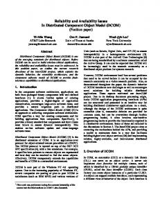
STATE-OF-THE-ART IN MOBILE AGENTS AND MULTI-ROBOT AREA COVERAGE Distributed computation, communication and coordination have been occupying the center-stage in Computer Science ever since the success in networking. Research and Development in distributed computation, information, storage and control resulted in tremendous interest in “Actors” or “Robots” related research. Coincidentally, all these areas suggested the “concept of a mobile agent” in their respective arena. One such field of study is the Mobile Robot based System, used for a variety of tasks that require navigation, exploration and coverage among several other interesting and demanding dimensions. Besides, the knowledge about the distributed environment varied from no knowledge to full knowledge in various studies. Of these, area coverage using multiple robots is central to several applications such as robotic de-mining, surveillance, robotic rescue and covert applications. Figure 2.1 depicts the historical developments in Distributed computing and the evolution of multi-robot area coverage.

Distributed Computation, Coordination, Communication

Computation

Information

Actors or Robots

Storage

Control

Mobile Agents …

…

Multi-Robot Systems

Navigation

Coverage

Exploration

…

…

Figure 2.1 Evolution of Multi-Robot Area Coverage Problem

In this chapter, we survey research in multi-agent systems at a macro level and critically analyze the work related to multi-robot area coverage at micro level. This chapter

11

concludes by highlighting some of the outstanding research challenges, which are examined in this thesis. Sycara [Kati98] discusses challenges in the design of multi-agent systems and states that formulating, decomposing and allocating tasks and synthesizing results are important in understanding multi-agent systems. Further, communication techniques and types of interaction among the agents must be explicitly stated in order that the system so designed remains simple. While the languages and protocols for achieving interactions affect the performance of the multi-agent system, they are left to designer’s choice and they often depend on (and are influenced by) the application at hand.

2.1 Coordination in Multi-agent Systems: A Survey A new direction for research in multi-agent systems is in the area of cooperative multiagent systems. Cooperative frameworks for multi-agent systems that are found in literature are of two basic kinds; namely, the Joint-Intentions [Cohe90] framework and the SharedPlans [Gros96] framework. In Joint-Intentions, a team of agents jointly commit to achieving a persistent goal and in SharedPlans, a coordinating agent helps schedule the tasks for the other agents. In yet another cooperative framework, STEAM [Tamb97], a combination of Joint-Intentions and SharedPlans are implemented. In-depth study of coordination and cooperation in multi-agent systems is provided in [Less99]. The author reckons that challenges in achieving coordination among cooperative agents working with local information are as follows: •

Limited computational capabilities and communication bandwidth makes it infeasible for large data transfers.

•

Heterogeneity among agents makes the task sharing complicated.

•

Dynamic environment and associated stochastic nature often makes it impossible to anticipate resource requirements and coordination needs.

12

The author reiterates that in order to develop efficient multi-agent systems, one must explicitly account for the costs incurred for the benefits and costs of coordination in a quantifiable way. In [Tamb97], the author proposes a new coordination framework typically suited to continuous, dynamic and unpredictable domains. The work highlights how an agent must inter-twine modeling the behavior of other agents, in order to anticipate what to do next. In [Davi02], the authors provide a comprehensive analysis of all teamwork theories and the computational complexities. This work decomposes the complexities in terms of use of communication and levels of observability.

2.2 Multi-agent Systems as Software MobileVCE, MOHICAN & the GAIA Methodology: The authors present a flexible coordination framework [Exce05] that allows agents to commit/decommit midway through a task by reasoning on their commitment levels and imposing penalties. Having committed to a coordinated task, the framework allows the agents to choose from within a fixed list, the most appropriate coordination mechanism to carry out the task. In case an agent needs to travel to another location to complete the task, an incentive is given for the time steps taken to reach that location. Every commit action is associated with expected reward and probability of success. The agent then chooses a task that gives the best reward. In [Jenn99], the author stresses on the need for a Social layer over the (decisionmaking) Knowledge layer, so that the system behavior and conceptual structures can be studied by abstracting the implementation details and the interaction protocol details. ExcelenteToledo [Exce01] outlines different techniques to switch between various coordination mechanisms dynamically by setting up a dynamic coordination evaluation model. On evaluation, the agent chooses the then best mechanism to coordinate on future tasks until next evaluation [Exce04, Exce03, Exce02].

Interaction Frames - InFFrA: In [Rova03], the authors propose a domain-independent communication framework which associates semantics to the messages based on the 13

agent experience. While the framework assumes ability for each agent to observe and record all interactions and predict future interaction trajectories [Rova04], it is observed to be a contingency-reducing and autonomy-respecting protocol. The authors then propose learning methods [Rova04] to adapt to unknown environments and learn to coordinate by communication. Here, the communicative interactions are modeled as MDP (Markov-Decision-Process). They define an implicit hierarchical architecture to validate the same.

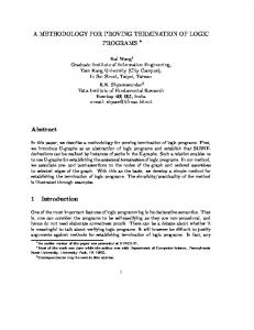
Agent-Oriented Programming: Agent-Oriented Programming (AOP), shown pictorially in Figure 2.2, is a relatively new programming paradigm introduced by Shoham that “promotes a societal view of computation, in which multiple agents interact with one another” [Yoav93]. At the conceptual level, this view presents AOP as a specialization of the Object-Oriented Programming (OOP) Paradigm. This framework supports the development and delivery of agents that use the reasoning

models

discussed in the previous section.

Further,

by

presenting the decision-

Object Object Engine

Agent Agent Engine

Figure 2.2 Agent Oriented Programming

making machinery as a generic agent interpreter the agent is reduced to a lightweight software entity (mental state + program) that is easily transmitted over a network. Finally the relationship between a class and an agent is of paramount interest in terms of the design of agents. This relationship supports the use of design patterns in the agent development process and promotes the reuse of agent code.

2.3 Beliefs-Desires-Intentions Framework (BDI Framework) Belief-Desire-Intentions: Majority of research in this area has been concerned with developing practical deliberative reasoning models. Perhaps the most successful attempt at constructing such models has come from the application of a mental state comprising a

14

set of mental attitudes such as beliefs, obligations, goals, and commitments. Within this field, a consensus mental state has emerged, the Belief-Desire-intention (BDI) architecture. In this terminology, an agent can be identified as having: a set of beliefs about its environment and about itself; a set of desires which are computational states which it wants to maintain, and a set of intentions which are computational states which the agent is trying to achieve.

Joint Intentions: While past research has comprehensively dealt with multi-agent systems, coordination mechanisms, and communication as means of coordination, no work has really gone into understanding the coordination infrastructure required for analyzing cooperative multi-agent systems working in real-time environments. In our work, we intend to address this challenge and develop an adaptable architecture for coordination as well as communication protocols needed for tackling a range of cooperative mobile multi agent tasks.

2.4 Coordination in Multi-Robot Systems Subsumption Architecture: The Subsumption Architecture or the Brooksian Architecture views a robot task as a vertically decomposable set of parallel computational modules interacting with the physical sensors to obtain input and process them to control those using actuators. This architecture provides a tight coupling between the Sensors and Actuators for a Mobile robot separated by a thin line of subtle rules that forms the reasoning layer.

Noreils, Mataric, Batalin, and Parker describe different approaches for mobile robot coordination with varying initial spread of the agents and propose heuristics that address the area coverage problem. Of these, Parker [Park02] and Noreils [Nori93] look at the problem in a distributed setting using only local sensory information. Mataric [Mata97] and Batalin [Bata02] have described various algorithms for distributed coverage of a given area using several mobile sensors that can spread out to optimally position 15

themselves balancing out maximum coverage while maintaining certain level of connectivity with the sensor network. A cost function C is assumed to mimic the functional requirements of the application. The inter-sensor distance is based on signal strength and the sensors move farther apart from a given initial placement until an optimal value of the cost function is obtained. Farinelli et al. [Fari04] present a comprehensive survey of multi-agent robot coordination techniques and classify them based on the coordination and system dimensions; where coordination dimension takes care of cooperation, knowledge, coordination, and organization – whereas system dimension refers to tackling issues related to communication, team composition, system architecture, and team size. The work in [Cao97] provides a classification of the multi-agent robotics domain along the dimensions of communication, computation and other capabilities. Communication is itself classified along range, bandwidth and topology. As the robots do not possess significant capabilities, some work in literature has viewed at ant-like movements [Kube00] using pheromones as a kind of sensory information to enable the following robot to sense the presence of another earlier at a location. In such works, a leader is elected and the remaining robots follow the leader. But such techniques do not suit coverage problems where all agents need to distribute themselves rather than follow a particular agent. In [Bata02], a coverage algorithm for dynamic area coverage using mobile sensors and landmark stationary nodes has been demonstrated. This work assumes the area to be a planar and devoid of any obstacles.

2.5 Robotic Exploration and Coverage Choset and Pignon [Chos01] introduce a new decomposition known as the Boustrophedon which works without a priori knowledge of the region unlike Morse function decomposition [Miln63]. “Boustrophedon” is a term used to describe the manner in which a bull or a yak ploughs a field. Figure 2.3 shows a sample Boustrophedon path

16

for single robot coverage of a given area. The challenge in this approach is to minimize the number of turns required by the robot at each boundary or obstacle without altering the rate of coverage.

Figure 2.3 Boustrophedon Path

Huang [Huan01] presents an approach to minimize the number of line sweeps in covering an area. The work achieves this goal by minimizing the sum of sub-region altitudes (a measure of the relative sweep directions). The algorithm employs planar line sweep to divide the coverage region into monotone sub-regions. The work also claims that decomposition of the region is not independent of the sequence in which robot must visit the cells and cover the area. Mathematically, the equation to be optimized is given by: S (θ) = dp(θ) + Σ dhi(θ)

… (2.1)

…where dp(θ) is the diameter function and dhi(θ) is the hole I of dp(θ) and θ is the angle of rotation. Acar et al. [Acar01] describe a single-robot coverage algorithm that makes use of prior knowledge about the positions of obstacles and then generates a line sweep through the space. The line sweep generated is according to critical points of Morse functions [Miln63] to decompose the regions into exact cells as illustrated in Figure 2.4. The line sweep is generated parallel to the tangent at the starting point for the robot. Acar et al. claim that the critical points are generated only at the boundaries of robot’s free space. According to this algorithm, once the starting robot location and the obstacle positions

17

are known, the exact cell decomposition is automatically computed and then a simple search algorithm is employed to determine a walk-through of the cells, which is represented as an adjacency graph, to cover the area.

...

Cell 2

Cell 1

Cell 3

Figure 2.4 Boustrophedon Decomposition

Acar et al. [Acar01] also present a complete sensor-based coverage algorithm using exact cellular decomposition. This work assumes a priori knowledge about mine patterns and uses a probabilistic method to identify them with imperfect sensors. Morse functions [Miln63] are used to decompose the region into cells and the generated critical points occur only at the boundaries of robot’s free space. Mines, laid out in regular patterns, are assumed to be characterized by 6 parameters and these are estimated using the Bayesian estimation theory. Butler et al. [Butl99] propose an algorithm for incremental cellular decomposition called CCRM to perform coverage of an area using contact sensors. The robot always executes a straight-line trajectory which is comparable to the line-sweep algorithm for coverage. After each straight line trajectory is executed, a new trajectory is chosen based only on the region C and the robot’s current position. This decision is governed by a set of rules that guarantee coverage in all possible conditions. Completeness of this algorithm has been shown by modeling it as a 3-state FSA with no infinite loops and describing all ways of evolving region C under CCRM.

18

Zelinsky et al. [Zeli93] introduce a distance transform method to determine paths of complete coverage to reach a single goal from its starting location. This is an offline technique and assumes prior knowledge about the coverage region and the positions and shapes of the obstacles. The distance measure (in terms of cell movement) is calculated and a wavefront is generated which marks all neighboring points around the goal with 1 and the cells surrounding those with 2 and so on. The distance transform technique for complete area coverage is illustrated in Figure 2.5. This distance measure is back propagated until the start location is reached. Then the robot begins by traversing all regions of equal distance and then proceeding inwards. The transform describes a numeric potential function which repels all obstacles and boundaries.

7 7 7 7 7 7

6 6 6 6 6 7

5 5 5 5 6 7

4 4 4 5 6 7

3 3 4 5 6 7

2 2 2 2 2 3 4 5 6 7

2 1 1 1 2 3 4 5

2 2 2 1 1 2 Go 1 2 al 1 1 2 2 2 2 3 3 3 4 4 4 5 5 5

Figure 2.5 Zelinsky’s Distance Transform

Wong and Macdonald present two performance metrics in [Wong02] for measuring the efficiency of area coverage using the support of computer vision. Assuming that the entire task can be video graphed, the paper identifies percentage area covered and distance moved by the robot as two metrics which are computed using a series of difference images with respect to a reference image. The reference image is initially taken before the task begins and this provides complete knowledge about the environment to the robot during coverage. Wong and Macdonald [Wong01] present a new approach called topological maps which uses exact cell decomposition information. The algorithm assumes the presence of natural landmarks for localization and a connectivity graph to represent the adjacency relations between sub-regions is constructed. The authors also claim that if the sub-region is intersected at 2 points, then the region can be fully covered using a zigzag pattern which is parallel to sweep line. The algorithm is modeled as a 3 – state FSA represented by

19

Normal, Boundary and Travel states. It is assumed that the robot always begins at a boundary. Gabriely and Rimon [Gabr01] present a theoretical study on coverage approaches for providing optimal paths in grid-like regions with exact cellular decomposition. The region with exact decomposition is represented as an adjacency graph and the optimal path for coverage is obtained for a single robot starting at a particular node. The work claims to provide exact-once coverage and has 3 versions. The first one is an off-line algorithm which assumes complete knowledge about the region and covers it in O(N) time where N represents the number of cells. The second version is an on-line algorithm, also covers the region in O(N) time without any prior knowledge but requires O(N) memory to store the covered locations details. The third version is an on-line version which functions in an ant-like fashion using pheromones with no prior knowledge and requires on O(1) memory to cover the region in O(N) time. In Rekleitis et al. [Rekl00], a tightly coupled algorithm for area coverage using 2 mobile robots is described. The work keeps the two robots in closely-coupled coordination and each is always in line-of-sight of the other. At any time, only one of them may explore while the other is stationary and functions as an artificial landmark. If, during exploration, line-of-sight view is lost, them the mobile robot backtracks and the roles are interchanged. The essential operation in coverage here is triangulation and the robots explore one triangle of free space area at a time. This work claims advantages of introducing artificial landmarks as being detectable and unambiguous. The algorithm assumes a priori knowledge of the environment and the triangulated regions. Butler et al. [Butl01] present a cooperative sensor based coverage algorithm using multiple robots based on CCRM is described which runs independently on all robots. CCRM decomposition algorithm for rectangular area is shown in Figure 2.6. Coverage and cooperation are totally decoupled which ensures a simpler completeness proof. This work uses the CCRM algorithm [Butl00] which incrementally constructs a cellular decomposition of the region and also uses a component called the Overseer which

20

integrates incoming data from other robots in region C. The Overseer operates in such a way that CCRM may continue without being aware that cooperation has occurred.

Y

X

Figure 2.6 Cell Decomposition Using CCRM

Simmons et al. [Simm00] describe a mapping algorithm which is an on-line approach to likelihood maximization using hill-climbing to find maps maximally consistent with sensor data are presented. Each robot processes its own laser data and a central mapper integrates the local maps to create a consistent global map. Each robot estimates expected information gain and associated costs for traveling to various locations and then forms bids which describe these estimates. A central evaluator receives all these bids and assigns the various locations in a manner that maximizes the global utility. The work assumes that the world is static and that it has a priori knowledge of starting positions of all the robots. By its assumption that the world is static, this work is restricted to domains with small number of robots as a large number tend to render the world dynamic. For this algorithm to work efficiently, all robots must possess the knowledge of the relative pose of one another and also have access to high bandwidth communication to exchange data.

Zlot et al. [Zlot02] present an approach to multi-robot exploration & mapping using market economy architecture for maximizing information gain and minimizing costs. The system is robust to communication failures and dynamic inclusion and failure of robot team members. Each robot which senses the area estimates a map M of the region and communicates the same. An agent called the Operation Executive mimicking the user’s (application) interests, awards a revenue to that robot based on revenue function R. A cost function C which is a mapping from set of resources used to the positive real number 21

function is also calculated and awarded to that robot. Depending on these two inputs, the robot computes its profit as the difference between revenue and cost and then chooses the locations which minimize its costs while maximizing profits. As the robot makes its bid public, other robots are allowed to enter into an auction and bid for that location. If a robot receives a bid better than the one it proposed, it relinquishes its claim for that location and proceeds to the next bid or to explore other locations. In Sheng et al. [Shen04], a totally distributed coordination algorithm for exploration using a distributed bidding model is explained. It assumes communication between robots to be range-limited and accommodates the same by using a nearness factor λ in the coordination algorithm. The algorithm is based on frontier cell exploration described in [Yama97] and maintains a gain function g which varies as a function of information gain i, distance to frontier cell d and nearness factor λ:

g = ω1i – ω2d + ω3λ

… (2.2)

… when w1, w2, and w3 are constant

The nearness factor ensures that no robot is isolated and that robots move in subnetworks which are always in communication. When a robot places a bid and finds no response within a preset time-bound, the robot declares it winner and proceeds with the task. The robot behavior is modeled as a 3-state FSA, viz., mapping, bidding and traveling. Whenever the mapping state is complete, a robot communicates that information to other robots within the sub-network and then it begins the bidding process. The work is contrasted with work reported in [Simm01] who propose the use of a central agent to evaluate the bids. According to this algorithm, when a terrain is identified, the robot evaluates certain criteria to check if it can explore the area. If the area is too small of if the robot is too tiny, it may transfer the task to another efficient robot. [Zlot02] present a distributed scalable bidding strategy based on market economy which is reliable and robust to one or more robot failures.

22

Solanas and Garcia [Sola04] present an unsupervised clustering algorithm that partitions the unknown space into as many clusters as the number of mobile robots. The partitioning is performed on-line as new regions are identified. The assignment of regions to the various robots is based on bids that are estimates of information gain traded-off against traveling costs to that region. The work assumes that robots are aware of the global state at all times and the algorithm attempts to spread the robots to explore their assigned cells. This work uses a regular 2D occupancy grid and each robot moves to its least cost frontier cell [Yama97] and penalizes other frontier cells within its sensor range. The new regions are partitioned using K-means least squares partitioning algorithm and the assignments are maintained throughout the exploration. In ant-robot based terrain coverage [Koen01], simple robots with minimal sensory capabilities perform at least once-coverage or continual coverage of an unknown terrain. The terrain is exactly decomposed into cells, each of which is the size of a robot. The work assumes that multiple robots may visit a single cell simultaneously without hindering the coverage path of other robots. Robots move in perfect synchronization during coverage without communicating with one another but rely on pheromone trails left by other robots earlier at that location. The action selection mechanism is based on an arbitrary function used to select the action that minimizes some cost function known a priori. Kube and Bonabeau have also looked at ant-like movements for robot exploration [Kube00] where a leader is elected and the remaining robots follow the leader along some arbitrary path. But the objective function in such techniques is either at least once coverage or continual coverage of a terrain, both of which are not advocated by our thesis. Our work attempts to avoid revisits to cells in the terrain whenever possible.

2.6 Need for Simplicity and Scalability In this chapter, we surveyed the evolution of the Multi-robot Area Coverage problem since the advent of distributed computing and coordinating multi-agent systems. We analyzed various coordination modes and elicited new directions for research in multiagent systems. Related frameworks in existence (SharedPlans, Joint-Intentions, STEAM,

23

InFFrA, BDI, etc.) in literature were also presented. Recent work in coordinated multirobot systems conclude that a multi-robot system can be classified along coordination and system dimensions, taking into account the knowledge level, communication requirements and system cost. Robotic exploration and coverage have emerged as key applications in the context of multi-robot systems and several research results were reported. Exploration focused on optimal path determination for robots to spread out and explore a given unknown area, while coverage focused on minimizing the system overhead while exhaustively visiting all locations in a given area. There appears to be a general consensus that coordination is the key to optimizing system utilization and this required effective communication techniques to be employed [Kati98, Less99, Exce01, Exce03]. In the next chapter, we introduce the multi-robot area coverage problem and propose a family of algorithms for minimizing the system overhead in coverage for different contexts. Some key requirements in achieving this endeavor involve the development of a methodology for solving Multi-Robot Area Coverage through Communication & Coordination and develop a class of light-weight algorithms for Multi-Robot Area Coverage to be integrated with simple mobile robots. Implementation of this solution methodology in a real scenario also requires that we design suitable Coordination Architecture for communication among mobile robots for performing the area coverage. Moreover, it is essential that we implement the solution using our custom-built MultiRobot Area Coverage Simulator (with Graphical User Interface) to understand the intricacies involved in a holistic sense. Finally, we design suitable simulation experiments to understand the behavior of these algorithms for varying coverage area and robot team sizes.

24

Chapter

3

ALGORITHMS FOR MULTI-ROBOT AREA COVERAGE PROBLEM 3.1 Exploration and Coverage Consider a scenario where a bomb squad is in operation to detect and diffuse all the explosives in an unknown territory to enable the battalion to move freely. This task requires that a bomb squad move ahead of the battalion to comb the entire area and diffuse all explosives. Ideally, while performing a combing operation, the area under consideration should be covered with a single forward sweep. However, in practice, a few back-and-forth movements will be unavoidable, resulting in repeated visits to a location, thereby increasing the overlap. An example of such a bomb squad is a team of robots working in close coordination. The requirements placed on the squad in achieving the above task are the following: • •

The squad must analyze the terrain and distribute work in such a fashion that it can be completed in minimum time. All robots should do near equal work

This example underlines the need for communication between the team of robots for area coverage tasks. The communication facility should enable message passing between the robots; the messages themselves should be selected / sequenced based on a protocol specifically designed for this purpose. A coverage area can be visualized as a grid consisting of M × N cells, each of square geometry and identical size. Representing an area in this form is called the vacancy grid representation. In this representation, a zero denotes free unexplored space and a nonzero value denotes either a covered cell or obstacles, as the case may be. Typically, positive numbers are used to represent robot visits and negative numbers are used to represent obstacles. A team of M homogeneous mobile robots, which can communicate with each other, is deployed for coverage. When the robots communicate, they exchange 25

‘state’ information. We assume that the robots have the capability to sense the locations (or cell) and the boundaries when they reach them. The problem is to develop a distributed algorithm that directs the robots to cover the area effectively. In this paper, we focus on minimizing the number of revisits to the cells and measure this using the overlap_ratio. The main challenge is that the area to be covered is unknown to the robots as they possess only limited visibility. The robots often have knowledge only about the extent of this area and can sense/detect the adjacent cells. It forces the robots to take coverage decisions based on their view of the environment. It is therefore essential that the team of robots spread out as far apart as possible in the initial stages and cover ‘nearby regions’ with minimal external input. External input in such situations is available only through messages containing ‘state information’ sent by other team members. Hence, robots communicate with each other periodically to synchronize and possibly take the optimal decisions. Of course, there is an implicit assumption that the robots are selfless in discharging their duties. It is also true that the robots do not have complete information of the environment in which they perform the area coverage. How do we frame this problem? Given an area, we employ a group of N robots to cover the area. The area can be divided into integral number of smaller shapes, again of regular geometry. It is required that the robots sweep the area completely with minimal repetitive scanning in the shortest possible time. In order that coordinated task completion is achieved, it is necessary to ensure that robots resolve conflicts in finite time. To facilitate this, we assume that all robots are equally capable and uniquely addressable. Each robot also knows the total number of robots in the team used for the area coverage task. Further, we assume that the robots are aware of the territory boundaries and can communicate, when required, with other robots at all times. The state information of a particular location can be obtained by a robot in two distinct ways. Either, the robot possesses additional sensors with computation capability to scan a

26

location and assess if it requires coverage or the robot can communicate with other robots to find out if the location has been covered. In the latter, if the area has been covered, then the robot which covered the area must store and recall this information and such a solution should be scalable to large number of robots. Every robot actively interacts with its environment that periodically evaluates its performance and provides a feedback. The robots also communicate to ensure that all other robots are aware of the regions covered and the regions remaining to be covered. For a given initial positioning of the robots, we use the Manhattan Distance (represented by dij) as a measure of the distance of roboti from another robotj. Intuitively, we feel that increasing dij allows a robot to maintain a reasonable number of future directions open that allows easy movement for coverage without cell overlap or collisions. Whenever dij is small, the robots are forced to move along the only available directions when overlap is critical. Such movements often lead to unequal coverage as it affects all future movements as well. In the next section, we describe the role of coordination and communication in Multi-robot systems and the need for a functional architecture for Multi-robot systems when applied to Area coverage problems.

3.2 Role of Coordination and Communication Coordination in multi-robot systems can be achieved either by centralized arbitration or by distributed arbitration with global knowledge of the system. Centralized arbitration requires a central arbiter, who always has global knowledge of the system and its environment and can control all robots directly. This framework makes an implicit assumption that there exists a hierarchy among the robots and that all robots are aware of its existence. This also requires that all robots remain in constant communication with the central arbiter, either directly or indirectly. There are two issues arising out of such a centralized design. In order to ensure that available resources are effectively utilized, the central arbiter needs to be a robot, just as any other, taking part in covering the area. But this entails arbiter performing more work than other robots which could drain the power

27

faster if it is battery-operated. One solution is to use a time-based sharing of central arbitration among the robots to ensure that all get equal work and share the load. In addition, each robot, when it becomes the central arbitrator must have the global system information to guide the other robots in the right direction. Suppose the arbiter is not a robot, then this would

Centralized Arbiter

require additional infrastructure for coordination which may not be suitable to all situations. While this is a fairly simple coordination technique to realize, it will turn out to be too limiting as the functioning of the system is critically dependent of the arbiter and its knowledge of the system. In our example one of the robots has to play the role

Agent

of central arbiter. The central arbiter decides on Figure 3.1 Centralized Coordination the optimal work to be done by each of the robots at every step and communicates the same through messages. Again, communication would warrant the need for sequencing since a single arbitrator must communicate with all subordinates. In the context of area coverage with large number of robots, the decision-making process becomes very tedious and results in significant delays to the area coverage application. The messages and associated communication will result in a star topology with two-way communication as illustrated in Figure 3.1. Distributed arbitration with global knowledge assumes that every robot knows exactly what it is doing, where

Any-to-Any Communication

the others are, what they are doing, and what needs to be achieved. Distributed systems

with

global

knowledge

exchange

state

information

periodically.

Usually,

the

information

consists

of

state current

Agent

Figure 3.2 Distributed Coordination

28

location and ‘proposed’ future location resulting from the individual ‘motion prediction’ algorithm. When such global information is available, each robot can effectively coordinate, implying that they can work towards avoiding ‘conflict’ in the ‘proposed’ future locations. Such algorithmic decisions – heuristic or otherwise – can be tuned to cover the area faster with minimal overlap. The successful execution of such distributed algorithm requires that each robot has the ability to communicate messages to all other robots, as illustrated in Figure 3.2. Communication: The functional block diagram depicting the requirements of a MultiRobot application scenario is shown in Figure 3.3. As mentioned earlier, Area Coverage is integral to applications involving multiple robots and coordination among the robots. For example, to cover a given area using multiple robots, one needs the following: •

Algorithm to decide the next step(s) to cover – such a decision needs “awareness” on the part of the robot about the “environment” and “context”.

•

Messaging facility which enables coding of “environment” and the “context” by each robot and ability to communicate the same to the other robots through appropriate communication protocols.

•

Network Technology Support for physically communicating the messages to the other robots with an appropriate choice of topology (star, tree, mesh, etc.) and mode (unicast, multicast or broadcast).

Application (Area Coverage) Algorithmic Decisions Context Sensitive Input

Context Sensitive Output

Messaging System Architecture Network Technology Support Figure 3.3: Functional Block Diagram of a typical Multi-Robot Coordination Scenario

29

In area coverage applications, each robot takes part in the distributed discovery of the next position through exchange of messages. Each application-level action is translated into actions to be performed by each robot. In order to achieve this, the coordination algorithm for coverage must take each robot through a series of steps such as localizing the robot, selecting the next action and communicating the same to other robots. This calls for direct communication between robots in order to maintain global knowledge. Besides, area coverage application requires that such transitions by each robot should result in covering the entire area – that too with a rider that the overlap in coverage is maintained near zero. In order to conform to these stringent requirements of the application, the algorithms (that execute within each robot) should decide the next state of the robot based on a contextsensitive input. This has led to the discovery of several algorithms which suit different contexts. To enable the robots to participate in the context-sensitive algorithmic decision making, messaging system architecture is essential. Typically messaging system architecture consists of the definition of different types of messages to suit (different) contexts and their exchange sequences or protocols to realize the meaning associated with the algorithmic actions. All these require a set of assumptions that are valid in the framework used in this thesis. In the sequel, we describe the Area coverage problem, the scenario, the assumptions, their impact and the performance metrics used.

3.3 Assumptions and their Impact As we proceed to solve the multi-robot area coverage problem, it is necessary to highlight the assumptions made in this thesis about the nature of the problem and its solution. The robots must communicate with each other periodically and they communicate before every action is chosen in order to coordinate their actions and minimize overlap. We also assume that these robots can sense the boundaries and can avoid actions that take them outside the grid.

30

Since all robots need to be aware of a particular robot’s state and intention (next step action), all robots communicate to the team and all communication are broadcast in nature. In order to be able to communicate any useful information, the robots must be able to sense the information from their respective environment. Each robot should be capable of localization to identify itself with respect to the coverage grid. While communicating the state information, it will be inappropriate if each robot senses the state information of the grid with respect to itself. This could result in anomalous interpretation of the state message by the other robots (during communication), unless there is a “global director”. Hence it is essential that all robots share a common frame of reference and all information sensing be done with respect to that reference. To verify each chosen action as appropriate (which do not result in robot collisions), a robot communicates this information to all the other robots and obtains a feedback on its validity. It is necessary that the robot is aware of the number of responses that it has to wait for. This indicates that the robots also require knowledge on the number of robots deployed for coverage. In the unlikely situation that two or more robots disagree on a decision, we need a mechanism to break ties quickly and proceed with coverage. Assuming the robots are able to distinguish each other among themselves based on some IDs, in our work we assume that during ties, the robot with the smallest ID always wins. This implies that during a tie, the robot with a smaller ID gets precedence over the other(s) and is allowed to retain its decision. The other robot(s) then change(s) its decision(s) by selecting a different action for movement. This assumption ensures that in the worst case when all robots attempt to move into one particular cell, repeatedly, the number of robots involved in the tie reduces by one at each turn and is completely resolved in M-1 turns where M is the number of robots. In our experiments, each robot can perform four actions and therefore the tie will get resolved within three turns. In general, if the total number of directions of movement is greater than M, then resolving a tie requires M-1 steps. On the other hand, if the total number of directions for movement is less than M, then steps to resolve tie is Number of actions – 1.

31

For certain algorithms, we also assume that the robots can recognize covered cells onestep ahead to avoid selecting that action which takes a robot to that cell. To recognize cells covered by self, each robot uses a unique feature to mark all covered cells which may be used to recognize prior coverage of the region at some later point in time. To recognize all covered cells, we assume that the robots have an a priori understanding on a common feature used to mark all covered cells. Checking for this mark would provide the robot with the information whether that cell has been visited previously.

3.4 Performance Measure: Overlap Ratio and Steps for Complete Coverage In our work on area coverage, there are two important metrics that are used to measure the performance of our algorithms for covering a given area using a given team of robots. In most area coverage problems, it is sufficient for any one robot to visit a location and repeated visits do not provide additional value. Hence such back-and-forth movements by robots are detrimental to system performance. Figure 3.4 illustrates the overlap in the coverage of an 8x8 grid using 3 robots. Each robot is identified by varying shades of gray color and all cells with revisits are marked in black. Therefore, in given figure there are 5 cells in overlap across the 3 robots. We measure this factor to compute what is called the overlap-ratio. The overlap-ratio is defined as the ratio between number of revisits to cells to the total number of cells to be covered. This factor is bounded by zero at the lower end and is unbounded at the higher end. A value of zero therefore signifies effective and coordinated coverage with no revisits. Since, it is difficult to obtain complete coordination in a distributed setting, that too when only partial information is available, we attempt to get as close to this idealistic case as possible by successively tuning the coordinated movement strategy across different algorithms that we design. Overlap-ratio = Number of revisits to cells / Total number of cells in the area

… (3.1)

The other parameter, steps to complete coverage denoted by ‘S’, focuses on the speed of attaining complete coverage in a given setting. Having designed algorithms for coverage, 32

it is important, to study and understand the efficiency of coverage which is decided by the number of decision epochs required to perform coverage. Algorithms that progressively bring this value down provide significant enhancement on the performance efficiency and cost of coverage as communication cost reduces with each step. This is required as a metric to determine, in a given setting, the configuration of the robot team that must be used in performing coverage with highest efficiency in terms of cost and time. By configuration, we refer to the capabilities of the robots, number of robots and the algorithm to be used for a given area with specific application constraints.

4 3 2 5

1

Figure 3.4 Illustration of Overlap in Coverage

This was computed as (1/M) × (overlap-ratio + 1) × number of cells in grid, where M is the number of robots used in coverage. Since overlap ratio is bounded by zero on the lower end, the minimum number of steps to complete is given by, SMin = Number of cells in Grid / Number of Robots

… (3.2)

Clearly, this is in accordance to expectations as in perfectly coordinated movement, each robot covers exactly the same number of cells and there are no revisits. For a given grid, the number of steps required to complete is directly proportional to the overlap ratio and it is in our interest to keep that value as low as possible. For a fixed team size and varying grid sizes, it is interesting to note that the steps to completion are directly proportional to

33

the overlap ratio obtained. For a given coverage grid, increase in the number of robots provides significant speedup in terms of completion steps, which can help reduce the number of decision epochs and therefore communication costs. Having described the problem and the application scenario, we move on to describe a family of algorithms developed as part of our work. For evaluating the algorithms through simulation and to understand the impact of changes in grid sizes and number of robots in the coverage teams, and the algorithms on the efficiency of area coverage, we designed a simulator and designed specific experiments using the simulator. In the sequel, we describe the simulator and then the area coverage algorithms and their performance.

3.5 Multi-agent Simulator for Area Coverage The multi-agent area coverage simulator has a hierarchical architecture as shown in Figure 3.5. The architecture has 3 levels in its hierarchy, of which the first level, containing the M0 module, is responsible for integrating the coverage actions of the various robots. At the second level, an initiator module M11 controls initiation actions for the area coverage problem and is also responsible for spreading the robots either in a way which provides efficient coverage based on a heuristic or through random spreading. M0

Area Coverage Simulator M11

M12

M13

Coverage Module

Initialization

Output Generator

M21 Terminal Module

M22 Collision Avoidance Module

Decision Module

M31

D-Distance Calculator

M32

New-State Evaluator

M33

Modify State

Number of levels to follow

M34

Retain State

Figure 3.5 Multi-agent Simulator Architecture

34

The output control module M13 is responsible for calculating the performance measures for the coverage problem based on the strategy used and calls a GUI based interface that projects an animated view of the coverage pattern performed by the robots. This is a very useful module as it has often helped us in providing key insights into the working details of our strategies and helped us improve their performance. In this coverage simulator, the most important module is the coverage module M12 which permits the use of several heuristic based strategies to perform coverage of an unknown environment. While M11 and M13 are both terminal modules in that they do not expand themselves within the hierarchy, the M12 module calls the decision module M21 and the collision avoidance module M22. The algorithm for coverage is positioned within this module and its logic decides the sequence in which the M21 and M22 will be called. M21 handles the communication that needs to be done with the other robots of the team and is responsible for each robot selecting its next desired location through the list of valid actions permitted to it. On completion of this process, the control is transferred to the M22 module which checks for collision possibilities and if so, calls M21 if there is a need to alter decision. In the last level of the hierarchy, there are four modules, D-distance module (M31), Newstate evaluator (M32), Change new-state (M33) and Retain state (M34). M31 is the interrobot distance computation module which is called at every step of the coverage operation for each of the robots. The inter-robot distance measure is a positive and symmetric measure such that Distance (i, j) = Distance (j, i). This distance measure (computes the Manhattan distance between any two robots i and j, denoted by dij) reads 1 when two robots are adjacent to each other along either axis and is highest when they are at the diagonal ends of the grid. New-state evaluator is called whenever a robot chooses a new direction for motion in order to communicate this message to the other robots and seek their input on whether to proceed or not. A robot may object to such a decision whenever: • •

It proposes to move to the same location It has already covered that location

35

•

It has observed an obstacle at that location

When any one of these above three situations arises, the control is transferred to the M21 module that handles change of decisions and their communication. Change state is invoked when a robot proceeds with its intention of moving to a particular location from its current position while retain state keeps the robot at the same location if it gets surrounded by cells which are all covered or if it gets stuck at the boundaries of the coverage grid. The simulator maintains a global controller that monitors the progress of the coverage task and calls the termination module on completion of the same. The simulation of the area coverage problem is characterized: 1

Number of robots

2

Grid Size

3

Maximum number of permitted actions

4

Number of reruns of the experiment

5

Inter-robot distance variation

6

Coverage strategy

The coverage rate and the overlap ration are strongly dependent on the parameters listed above. It is observed that as the number of robots assigned to a given grid is increased, the overlap ratio decreases irrespective of the coverage strategy used. This may be attributed to the fact that M31 module forces the robots to take and maintain decision which keep them at least cells apart and in effect spreading them to achieve effective coverage. In the unlikely case that a robot gets stuck at a boundary or within a group of already covered cells, it is forced to retain its location until surrounding robots move away in order to avoid cluttering.

36

3.6 Algorithms and their Performance 3.6.1 Area Coverage in the absence of Complete Knowledge To perform coordinated coverage of a given area with multiple robots, it is essential to understand the behavior of these robots when there is no coordination or communication. As a result, each robot may visit a cell many times and many robots may simultaneously be present in a single cell. The robots continue to move in this manner until coverage is complete. The algorithm is given below and is called the NCC – No-Coordination-orCommunication algorithm. NCC Algorithm NCC Coverage Algorithm Given GRID of size (XMax, YMax) and M number of robots Initialize: Spread the Robots Randomly within the Grid Repeat while coverage not complete, For each robot, do Select a direction of movement at random Change state End of For-loop END of Algorithm

Figure 3.6 No-Coordination-or-Communication (NCC) Algorithm

Simulation Experiments for NCC Algorithm: Controlled experiments were conducted using the Area coverage simulator described earlier. The parameters – grid size and number of robots within the coverage team – were varied from 4 × 4 to 81 × 81 and 2 to 64 respectively. The experiments were done in two parts, reflecting the robot behavior as per NCC algorithm in smaller and larger grid sizes. The results are presented in Figures 3.7 – 3.9. Of these, Figure 3.7 gives the overlap ratio v/s number of robots plot for small grid sizes and Figure 3.8 and 3.9 give the same for larger grid sizes. The overlap obtained is the cumulative overlap ratio value across all robots in the coverage team. We assumed

37

that the initial placements of the robots are based on uniform distribution – that is all cells are equally likely – and that the placements of robots are independent events. The action selection mechanism uses uniform distribution to select the “next-step” for each robot. It is further assumed that the robots can move in four directions – north, east, west, and south.

Overlap Ratio Vs Number of Robots

Overlap Ratio

10 8

4x4 Grid 5x5 Grid

6

6x6 Grid 4

7x7 Grid 8x8 Grid

2 0 2

3

4

5

6

7

8

Number of Robots Figure 3.7 Performance of NCC algorithm for varying number of Robots (11% error margin)

Overlap Ratio 140

Overlap Ratio

120 100

27x27 Grid

80

32x32 Grid

60

64x64 Grid

40

81x81 Grid

20 0 2

3

4

8

16

24

32

64

Number of Robots Figure 3.8 Performance of NCC algorithm on large grids for varying number of Robots (11% error margin)

38

Overlap Ratio 140 2 Robots

Overlap Ratio

120

3 Robots

100

4 Robots

80

8 Robots

60

16 Robots

40

24 Robots 32 Robots

20

64 Robots

0 27

32

64

81

Grid Sizes Figure 3.9 Performance of NCC algorithm for given robot team size for varying grid sizes (11% error margin)

Observations and Inference: The overlap ratio remains within a band of 2 to 3 for small grid sizes and small number of robots. On the contrary, when we look at larger grid sizes, the overlap ratio significantly decreases from 120 to approx. 20 as we move from 2 robots in an 81 × 81 grid to 64 robots in a 27 × 27 grid. Besides, for larger grids the overlap ratio reduces as the number of robots increases. In fact, it is consistent where the grid size is very large. Perhaps, NCC algorithm is ideal for non-critical multirobot systems such as cleaning of the Empire State Building where the grid sizes and the robot team size are literally very large. It is simpler to implement and hence is likely to be least expensive to incorporate into automatic cleaning using robot technology. However, it is interesting to see the impact of coordination on overlap ratio as we move to the next algorithm. Coordinated Robot Movement Strategy: At each decision-making step, there is a current state and a next state as shown in Figure 3.10. The Motion predictor module maintains the list of current valid actions and a criterion to select the next best action. Each of the algorithms designed, differ in this selection criterion and they are successively refined to minimize the overlap. Every robot has an action sequence as shown in Figure. From its current state, a robot evaluates its available actions, selects and 39

communicates a decision to the team. If all the robots in the

team

accept

Already Selected action list

this

decision, the robot may

Current State

Evaluate action list

Motion Predictor

Communicate

Accept Action

Next State

move to the next state. If, however,

some

robot(s)

disagrees with the decision

All Actions Rejected

Figure 3.10 Coordinated Robot Movement Strategy

(such a robot has to be one with a lower robot ID), then the robot re-evaluates its actions. The process continues in the context of contention until either a valid action is chosen and accepted by the team or until all actions are rejected. On rejection, the action rejected is stored (temporary memory, like a cache) to ensure that the predictor module does not repeat the selection of the same action. If all the actions are reje cted, then the robot defers its decision by one step and stays in the same state. Only a robot that has the highest robot ID may need to defer its action selection owing to the assumptions detailed above. In such a case, other robots would move away and in the subsequent epoch the high ID robot is forced out of its location. This is the basis for decision-making at each step in the area coverage algorithms. OSC Algorithm The One-Step-Communicate algorithm requires each robot to communicate its current position and the next intended action to the team. All robots then compute the inter-robot distance between themselves. Since this strategy tries to separate two robots when a collision is expected, it provides more efficient coverage when compared with NCC algorithm where no a priori information is available.

OSC Coverage Algorithm Given GRID of size (XMax, YMax) and M number of robots Initialize: Spread the robots randomly in GRID. For each pair of robots (i, j), compute dij = Manhattan distance (robot i, robot j) Repeat while coverage not complete,

40

For each robot, do Let (x,y) represent the current coordinates of the robot Evaluate action choice list and select action such that it doesn’t reduce dij. Communicate with other robots to exchange state, action information. Compute the 1-step new states for all robots and check for overlap. If no collision, communicate accept message and change state On collision, omit action from action list. Re-evaluate action list If boundary along X-axis, select direction of which (YMax – y) or y is greater. If boundary along Y-axis, select direction of which (XMax – x) or x is greater. Else select an action with dij ≥ 2 and change state. End of For-loop END of Algorithm

Figure 3.11 One Step Communicate (OSC) Algorithm

Simulation Experiments for OSC Algorithm: The OSC coverage algorithm related simulation experiments were designed along the same lines as we have described earlier in this section in the context of NCC algorithm. The main difference, however, is that the simulator has motion predictor as defined in Figure 3.10 and the accept action in conformity with the OSC coverage algorithm. As a consequence, two robots will not be in the same cell in the same step. The results of the experiments are depicted in Figures 3.12 – 3.14.

Overlap Ratio

Overlap Ratio Vs Number of Robots 10 8 6 4 2 0

4x4 Grid 5x5 Grid 6x6 Grid 7x7 Grid 2

3

4

5

6

7

8

8x8 Grid

Number of Robots Figure 3.12 Performance of OSC algorithm for varying number of Robots (8% error margin)

41

Overlap Ratio 140

Overlap Ratio

120 100

27x27 Grid

80

32x32 Grid

60

64x64 Grid 81x81 Grid

40 20 0 2

3

4

8

16

24

32

64

Number of Robots Figure 3.13 Performance of OSC algorithm on large grid sizes for varying number of Robots (11% error margin)


Overlap Ratio

120

3 Robots

100

4 Robots

80

8 Robots

60

16 Robots 24 Robots

40

32 Robots

20

64 Robots

0 27

32

64

81

Grid Sizes Figure 3.14 Performance of OSC algorithm for given robot team size for varying grid sizes (11% error margin)

Observations and Inference: The overlap ratio remains within a band of 1.6 to 2.4 for small grid sizes and small number of robots, which is a marked improvement over the results obtained in the NCC algorithm case. For large grid sizes, the overlap ratio significantly decreases from 103 to approx. 20 as we move from 8 robots in an 81 × 81 grid to 64 robots in a 27 × 27 and 32 × 32 grids. Besides, for larger grids the overlap ratio reduces as the number of robots increases as we proceed from 8 robots to 42

64 robots in the team. In fact, it is consistent where the grid size is very large. Perhaps, OSC algorithm is ideal for non-critical multi-robot systems such as component classification and gathering in shop-floors, where the grid sizes and the robot team size vary from medium to large. It is simpler to implement and hence is likely to be less expensive to incorporate into automatic shop-floor robot technology. Deadlock Avoidance Mechanism In the following algorithms, we describe an explicit mode of behavior for the robots to avoid deadlock/trapped state. Such behavior is exhibited by a robot when it gets into such states and the goal under these situations is to get out of this state as quickly as possible. Deadlock/trapped state occurs when a robot finds itself in a cell surrounded by covered cells in all directions. Normal behavior (standard action selection according to the algorithm) in such states could lead to significant increase in overlap in the grid; the robot selects an arbitrary direction and moves linearly along this path until it reaches an uncovered cell. In comparison, ANT robot based terrain coverage does not have explicit notion of deadlock during robot movements. The objective of coverage is at least once or continual coverage of the terrain and permit robots to revisit cells as many times as necessary without penalty. Since such movements involve a penalty on the objective function in our work, we have explicitly called this behavior so. OSCSD Algorithm The next step is to build in the capability to recognize the local environment in each robot through sensor-implantation in the robots. Since each robot covers the area in its own way, it is fairly straightforward to integrate additional sensors in each robot to help detect and recognize cells covered by it earlier. The robot can therefore avoid those cells when a decision is taken. In this case, each robot marks a cell uniquely on its first visit to that cell. It evaluates its action-choices from an adjacent cell, recognizes its mark and avoids the action to selects another. But in the unlikely situation that a robot finds itself in

43

deadlock, it changes it mode of behavior into Deadlock avoidance and attempts to get out of this situation. In that situation, the main criterion is to release the robot rather than to avoid overlap. The algorithm called OSCSD – One Step Communicate – Self Discovery is given in Figure 3.15.

OSCSD Coverage Algorithm Given GRID of size (XMax, YMax) and M number of robots Initialize: Spread the robots randomly in GRID. For each pair of robots (i, j), compute dij = Manhattan distance (robot i, robot j) Repeat while coverage not complete, For each robot, do Let (x,y) represent the current coordinates of the robot Avoid previously covered cells by self; Identify and evaluate action list. Select action that doesn’t reduce dij Communicate with other robots to exchange state, action information. Compute the 1-step new states for all robots and check for overlap. If no collision, communicate accept message and change state On collision, omit action from action list. Re-evaluate action list On trapped, choose random direction and break-loop If boundary along X-axis, select direction of which (YMax – y) or y is greater. If boundary along Y-axis, select direction of which (XMax – x) or x is greater. Else select an action with dij ≥ 2 and change state. End of For-loop END of Algorithm

Figure 3.15 One Step Communicate – Self Discovery (OSCSD) Algorithm

Simulation Experiments for OSCSD Algorithm: The OSCSD coverage algorithm related simulation experiments were designed for the smaller grid sizes and along the same lines as we have described earlier. The main difference, however, is that the motion predictor in the simulator employs OSCSD in the decision loop. As a consequence, a robot will try and avoid revisits to the same cell unless trapped in deadlock. The results of the experiments are depicted in Figure 3.16.

44


Overlap Ratio

10 8

4x4 Grid 5x5 Grid

6

6x6 Grid 4

7x7 Grid 8x8 Grid

2 0 2

3

4

5

6

7

8

Number of Robots Figure 3.16 Performance of OSCSD algorithm for varying number of Robots (11% error margin)

Observations and Inference: The overlap ratio presents a divergent picture for small team sizes for all grid sizes. However, as the number of robots in the team increases from 2 to 8, the overlap ratio for grid sizes ranging from 4 × 4 to 8 × 8 converges to 2. As there is no marked improvement in the overlap ratio, simulation experiments were not conducted for higher grid sizes and larger number of robots. Perhaps the information that is gathered in OSCSD is insufficient to make any significant impact on the overlap ratio. This also underlines the need for communication between robots so that they exchange all the state information between themselves and take more informed decisions resulting in better performance. OSCARD Algorithm Since we deal only with homogeneous robots and the same algorithm executes in each of these, all robots cover a given cell in exactly the same way. Therefore a feature used to mark a covered cell by any one of these robots should be detected and recognized by all the other robots as well. In our next algorithm, we refined the OSCSD algorithm and came up with another algorithm called OSCARD – One Step Communicate – All Robots Discovery – that allows robots to recognize all covered cells in their path and therefore 45

avoid them when picking a direction to move. Though this is the ultimate goal of the work reported in our thesis, overlap could not be eliminated completely because robots are one-step greedy and myopic in decision-making. However, the algorithm shows significant improvement over the Self-Recognize (OSCSD) strategy. The OSCARD algorithm is given in Figure 3.17.

OSCARD Coverage Algorithm Given GRID of size (XMax, YMax) and M number of robots Initialize: Spread the robots randomly in GRID. For each pair of robots (i, j), compute dij = Manhattan distance (robot i, robot j) Repeat while coverage not complete, For each robot, do Let (x,y) represent the current coordinates of the robot Avoid ALL previously covered cells; Identify and evaluate action list. Select action that doesn’t reduce dij Communicate with other robots to exchange state, action information. Compute the 1-step new states for all robots and check for overlap. If no collision, communicate accept message and change state On collision, omit action from action list. Re-evaluate action list On trapped, choose random direction and break-loop If boundary along X-axis, select direction of which (YMax – y) or y is greater. If boundary along Y-axis, select direction of which (XMax – x) or x is greater. Else select an action with dij ≥ 2 and change state. End of For-loop END of Algorithm

Figure 3.17 One Step Communicate – All Robots Discovery (OSCARD) Algorithm

Simulation Experiments for OSCARD Algorithm: The OSCARD coverage algorithm related simulation experiments were designed along the same lines as we have described earlier. The main difference, however, is that the motion predictor in the simulator employs OSCARD in the decision loop. As a consequence, a robot will try to avoid revisits to all already covered cells (unless trapped in deadlock) based on the

46

communication capability which is built in for recognizing the global context. The results of the experiments are depicted in Figures 3.18 – 3.20.


Overlap Ratio

5 4

4x4 Grid

3

5x5 Grid 6x6 Grid

2

7x7 Grid 8x8 Grid

1 0 2

3

4

5

6

7

8

Number of Robots Figure 3.18 Performance of OSCARD algorithm for varying number of Robots (7% error margin)

Overlap Ratio

Overlap Ratio

50 40 27x27 Grid

30


20

81x81 Grid

10 0 2

3

4

8

16

24

32

64

Number of Robots Figure 3.19 Performance of OSCARD algorithm on large grid sizes for varying number of Robots (8% error margin)

47


Overlap Ratio

40

3 Robots 4 Robots

30

8 Robots 16 Robots

20

24 Robots 32 Robots

10

64 Robots

0 27

32

64

81

Grid Sizes Figure 3.20 Performance of OSCARD algorithm for given robot team size for varying grid sizes (8% error margin)

Observations and Inference: The overlap ratio remains within a band of 0.5 to 2.1 for small grid sizes and small number of robots, which is a marked improvement over the results obtained in the earlier cases. For large grid sizes Figure 3.21 Spiraling Paths

the overlap ratio varies from 5 to

20, which is a very significant reduction compared to earlier algorithms. Besides, we observe that the overlap ratio is nearly stable at very low values irrespective of the grid size and the number of robots in the team. This trend is nearly the same for all the experiments. This is mainly because in the OSCARD case overlap is possible only when robots are trapped within covered cells, as the deadlock is broken by random jump out of the trapped cell. This gives rise to a phenomenon, which we call “Spiraling Inwards”, as depicted in Figure 3.21. If this situation can be avoided the performance can still be better. This is attempted in the next algorithm. In spite of this Spiraling Inward Problem, OSCARD algorithm

48

is ideal for even critical multi-robot systems such as robotic de-mining applications. NJ Algorithm In our next algorithm called NJ - Neighbor Jurisdiction - we introduce the concept of jurisdiction that ensures that the robots maintain a certain minimum distance from each other at each step. Each robot fixes its center of operation and communicates the same to the team members. The robots would then follow a random coverage pattern for covering the cells within that jurisdiction without spiraling inwards. When two or more robots had to contend for coverage in the same region, it was arbitrarily decided that the robot with lower ID wins the bid. The other robots then choose random directions and move k steps away and then resume their normal coverage behavior. NJ Coverage Algorithm Given GRID of size (XMax, Ymax) and M number of robots Initialize: Spread the robots randomly in GRID. For each pair of robots (i, j), Compute dij = Manhattan distance (robot i, robot j) If dij < 2, push robot with higher ID 3 steps away Repeat while coverage not complete, For each robot, do Let (x,y) represent the current coordinates of the robot Avoid ALL previously covered cells; Select an action and cover cells in jurisdiction On trapped, choose random direction and break-loop If boundary along X-axis, select direction of which (Ymax – y) or y is greater. If boundary along Y-axis, select direction of which (Xmax – x) or x is greater. Else select an action with dij ≥ threshold and change state. End of For-loop END of Algorithm

Figure 3.22 Neighbor Jurisdiction (NJ) Algorithm

Simulation Experiments for NJ Algorithm: The NJ coverage algorithm related simulation experiments were designed along the same lines as we have described earlier.

49

The main difference, however, is that the motion predictor in the simulator employs NJ in the decision loop. As a consequence, any two robots maintain certain minimum distance (denoted by threshold) between themselves at each step during coverage. For the small grids, this threshold was kept at 25% of the side of grid and for larger grids it was fixed at 3 as it provided best results. The results of the experiments are depicted in Figures 3.23 – 3.25.


Overlap Ratio

5 4

4x4 Grid

3

5x5 Grid 6x6 Grid

2

7x7 Grid 8x8 Grid

1 0 2

3

4

5

6

7

8

Number of Robots Figure 3.23 Performance of NJ algorithm for varying number of Robots (7% error margin)

Overlap Ratio

Overlap Ratio

50 40

27x27 Grid

30

32x32 Grid

20


10 0 2

3

4

8

16

24

32

64

Number of Robots Figure 3.24 Performance of NJ algorithm on large grid sizes for varying number of Robots (8% error margin)

50


Overlap Ratio

40

3 Robots 4 Robots

30

8 Robots 16 Robots

20

24 Robots 32 Robots

10

64 Robots

0 27

32

64

81

Grid Sizes

Figure 3.25 Performance of NJ algorithm for given robot team size for varying grid sizes (8% error margin)

Observations and Inference: The overlap ratio remains within a band of 0.4 to 3.6 for small grid sizes and small number of robots, which is along the same lines as OSCARD with additional improvements for smaller grids and lesser number of robots and marginally higher values for overlap ratio in the case of larger number of robots. For large grid sizes the overlap ratio varies from 4 to 18, which is better compared to OSCARD. We also observe that the overlap ratio is nearly stable at very low values irrespective of the grid size and the number of robots in the team. However, the overlap ratio shows a rising trend for grid sizes 27 × 27 and 32 × 32 as we move from 2 to 64 robots in a team and the trend is concave for grid sizes 64 × 64 and 81 × 81 as we move from 2 to 64 robots. In the Neighbor Jurisdiction algorithm, if the initial positioning of the robots is such that the robots are clustered in one section of the grid, then these robots contend for positioning thereby increasing the number of messages exchanged between the robots significantly. This also resulted in bulk movements by robots (those which lost the bid) in certain directions. As a consequence, the overlap momentarily shoots high until the

51

requirements are met. This explains the phenomenon observed in the results of the simulation experiments associated with NJ algorithm which are reported in Figures 3.24 and 3.25. Notwithstanding the above, NJ algorithm is ideal for critical multi-robot systems such as rescue robotics and robotic de-mining applications.

3.6.2 Incorporating Memory into Robots A lot of messages are being exchanged between the team of robots at each decision epoch. To take advantage and make maximum utilization of the information, each robot may retain information (to store and recall) regarding the status of cells. A robot could use this information to locate and move to the closest uncovered cell when trapped. In other words, incorporating memory into these robots allows them to take informed decisions at each step by performing multi-step look-ahead to determine the most suitable candidate. Therefore this methodology allows the robots to intelligently decide on the next cell for coverage in a trapped situation and minimize the overlap. Each time, when trapped, a robot will refer to its memory and direct itself toward the closest uncovered cell thereby reducing overlap. OSCSD-m Algorithm In NCC algorithms, robots take independent decisions at each step and are not governed by communication between the robots. Through a similar argument, robots executing OSC algorithm work on a step-by-step basis and use communication only to avoid robot collisions. Since these two algorithms were designed to be memory-less, incorporating memory in those robots will provide no additional improvement in performance. On the other hand, robots executing OSCSD and OSCARD algorithms communicate to recognize and/or remember events and therefore can benefit by incorporating memory. In our work, we incorporated memory into each of the robots and tested the algorithms on grids of sizes 4 × 4 to 8 × 8. The algorithms for coverage on robots with incorporated

52

memory are given in Figures 3.26 and 3.30 and for the sake of uniqueness these algorithms are named OSCSD-m and OSCARD-m respectively.

OSCSD-m Coverage Algorithm Given GRID of size (XMax, YMax) and M number of robots Initialize: Spread the robots randomly in GRID. For each pair of robots (i, j), compute dij = Manhattan distance (robot i, robot j) Repeat while coverage not complete, For each robot, do Let (x,y) represent the current coordinates of the robot Avoid previously covered cells by self; Identify and evaluate action list. Select action that doesn’t reduce dij Communicate with other robots to exchange state, action information. Compute the 1-step new states for all robots and check for overlap. If no collision, communicate accept message and change state On collision, omit action from action list. Re-evaluate action list

On trapped, search for closest uncovered cell from memory and move to cell If boundary along X-axis, select direction of which (YMax – y) or y is greater. If boundary along Y-axis, select direction of which (XMax – x) or x is greater. Else select an action with dij ≥ 2 and change state. End of For-loop END of Algorithm

Figure 3.26 OSCSD-m Algorithm

Simulation Experiments for OSCSD-m Algorithm for Robots with memory: The OSCSD-m coverage algorithm related simulation experiments were designed along the same lines as we have described earlier. The main difference between OSCSD and OSCSD-m is that a robot remembers all cells visited. When it is trapped, it searches for the closest uncovered cell from its memory and moves to that cell. By this process of searching the robot performs a multi-step look-ahead in decision making. This approach enables the robots to avoid repeated visits to ‘trapped cells’. As a result, the performance of the algorithm should show marked improvement over the memory-less case. The results of the simulation experiments carried out for different grid sizes and varying robot team sizes are depicted in Figures 3.27 through 3.29a.

53

Comparison - Memory Vs No Memory (6x6 Grid) 20

10 8 6 4 2 0

Overlap Ratio

Overlap Ratio

Comparison - Memory Vs No Memory (4x4 Grid)

No Memory With Memory

2

3

4

5

6

7

16 No Memory

12

With Memory

8 4 0

8

2

Number of Robots

3

4

5

6

7

8

Number of Robots

Figure 3.27 Performance of OSCSD-m algorithm for 4x4 grid and varying robot team sizes

Figure 3.28 Performance of OSCSD-m algorithm for 6x6 grid and varying robot team sizes

Observations and Inference: When compared to the memory-less case, the overlap ratio drops significantly when the algorithm executes on robots with memory. While the “drop” is not perceptible for small grids (4 × 4 grid with 6 robots and beyond), it is prominent in larger grids. This is mainly due to the fact that the robots have ‘other options of cells’ to go to, when they are trapped. In order to understand the behavior of OSCSD-m algorithm better, we present in Figure 3.29b the percentage savings obtained in overlap ratio when robots with memory execute OSCSD-m algorithm as compared to robots without memory executing OSCSD algorithm. For grid sizes 6 × 6 and 8 × 8 having fewer than 6 robots, the savings are at least 50% when compared with the memory-less case.

54

25 20 15 10 5 0

100

Percentage Savings

Overlap Ratio


No Memory With Memory

2

3

4

5

6

7

80 4x4 Grid

60

6x6 Grid 40

8x8 Grid

20 0

8

2

Number of Robots

3

4

5

6

7

8

Num ber of Robots

Figure 3.29a Performance of OSCSD-m algorithm for 8x8 grid and varying robot team sizes

Figure 3.29b Percentage Savings in overlap ratio – With and without memory – Across Grid Sizes

On the contrary, for large team sizes, as coverage progresses, the possibility that each robot decides on its next move to a cell already visited by another robot increases. Such behavior is due to the lack of information about the movement and coverage by other robots and shows up as increase in overlap ratio in the results of our simulation experiments. OSCARD-m Algorithm To overcome the performance deficiencies exhibited by OSCSD-m, we design another simulation experiment based on the modification to OSCARD algorithm incorporating memory. OSCARD-m Coverage Algorithm Given GRID of size (XMax, YMax) and M number of robots Initialize: Spread the robots randomly in GRID. For each pair of robots (i, j), compute dij = Manhattan distance (robot i, robot j) Repeat while coverage not complete, For each robot, do Let (x,y) represent the current coordinates of the robot Avoid ALL previously covered cells; Identify and evaluate action list. Select action that doesn’t reduce dij Communicate with other robots to exchange state, action information.

55

Compute the 1-step new states for all robots and check for overlap. If no collision, communicate accept message and change state On collision, omit action from action list. Re-evaluate action list

On trapped, search for closest uncovered cell from memory and move to cell If boundary along X-axis, select direction of which (YMax – y) or y is greater. If boundary along Y-axis, select direction of which (XMax – x) or x is greater. Else select an action with dij ≥ 2 and change state. End of For-loop END of Algorithm

Figure 3.30 OSCARD-m Algorithm

Simulation Experiments for OSCARD-m Algorithm for Robots with memory: The OSCARD-m coverage algorithm related simulation experiments were designed along the same lines as we have described earlier. The main difference between OSCARD and OSCARD-m is that a robot remembers all the cells visited by itself and others robots in the team. When it is trapped, it searches for the closest uncovered cell from its memory and moves to that cell. By this process of searching the robot performs a multi-step lookahead in decision making. “Memory” of each robot carries complete coverage information at any point. As a result, the performance of the algorithm should show marked improvement over all the earlier cases. The results of the simulation experiments carried out for OSCARD-m algorithm for different grid sizes and varying robot team sizes are depicted in Figures 3.31 through 3.33a. Observations and Inference: The overlap ratio drops when the OSCARDm algorithm executes on robots with memory as compared to OSCARD algorithm executing on robots without memory. However, the ‘drop’ is perceptible only when the number of robots used for coverage is low, unlike the OSCSD-m case. In order to understand the behavior of OSCARD-m algorithm better, we present in Figure 3.33b the percentage savings obtained in overlap ratio when robots with memory execute OSCARD-m algorithm as compared to robots without memory executing OSCARD algorithm – this is to enable direct comparison with the OSCSD-m case described earlier. 56


10

10

8

8

6

No Memory

4

With Memory

Overlap Ratio

Overlap Ratio


2 3

4

5

6

7

No Memory

4

With Memory

2

0 2

6

0

8

2

3

Number of Robots

Figure 3.31 Performance of OSCARD-m algorithm for 4x4 grid and varying robot team sizes

Percentage Savings

Overlap Ratio

8 6

No Memory

4

With Memory

2 0 4

5

6

6

7

8

100

10

3

5



2

4

Number of Robots

7

80 60

4x4 Grid

40

6x6 Grid

20

8x8 Grid

0 -20

2

3

4

5

6

7

8

-40

8

Number of Robots

Number of Robots

Figure 3.33a Performance of OSCARD-m algorithm for 8x8 grid and varying robot team sizes

Figure 3.33b Percentage Savings in overlap ratio – With and without memory – Across Grid Sizes

We infer from the experimental results for larger number of robots, that the cells get covered quickly, often leading to traps. As a consequence, the robots are unable to find a ‘free cell’ to jump to. The robot takes a ‘random decision’ to move under such circumstances. Besides, we observe that linear increase in the number of robots did not necessarily result in linear increase in the number of traps. This may perhaps be the reason why we observe some cases having overlap ratios higher than their memory-less counterparts.

57

Overlap Ratio Vs Number of Robots (64x64 Grid)

20

20

16

16

12

W/O Memory With Memory

8 4

Overlap Ratio

Overlap Ratio

Overlap Ratio Vs Number of Robots (27x27 Grid)

0

12

W/O Memory 8

With Memory

4 0

2

3

4

8

16

32

64

2

Number of Robots

3

4

8

16

32

64

Number of Robots



When the algorithm was executed directly on grids of large sizes (27 × 27 and 64 × 64), the improvement was pronounced - over 60% drop in the overlap ratio for all cases. The results of these experiments are given in Figures 3.34 and 3.35. We infer that larger grids provide more opportunities for the robots to jump out of a trap situation and also reduce the possibility of overlap. These results indicate that OSCARD-m algorithm is suitable to critical applications like Robotic De-mining and Rescue Robotics where the areas generally tend to be very large and require large number of robots to cover the area in as short a time as possible.

3.6.3 Computing the Communication Overhead In each of the algorithms described above, we have mentioned that the robots communicate their decision to the team and will proceed only if all the team members accept the decision. Reject occurs when at least one robot in the team disagrees with the action chosen by another as it could potentially lead to two or more robots being present at the same cell at the same time. This situation by our assumption represents a collision and hence must be avoided. When a reject occurs, the affected robot discards that action and selects another from the remaining set of actions using a uniform distribution. Every reject requires the robot to re-obtain team’s approval by proposing a new action. It is 58

evident that rejects result in communication overhead for the team that affects performance. We conducted experiments to determine the number of re-decisions that occur during the coverage of a 6 × 6 grid for different number of robots. Each time the team rejected an action, the re-decision counter was incremented by one. The plot (See Figure 3.36) gives us the cumulative re-decisions across all robots in a coverage scenario averaged over 200 runs.

Number of Re-decisions

600 450 OSC Algorithm

300

OSCARD Algorithm NJ Algorithm

150 0 2

3

4 5 6 7 Number of Robots

8

Figure 3.36 Communication Overhead in decision making across algorithms for a 6x6 coverage grid for robots without memory

Observations and Inference: Robots executing the NCC algorithm, by definition, do not communicate and re-decisions in this algorithm occur only when the robots are at the boundaries. For other algorithms such as OSC, OSCARD and NJ, robots need to avoid cells where a collision can occur. In those algorithms, the contention is resolved by the lowest-ID robot getting priority in retaining its decision. We also observe that the number of collisions is significantly lower in above-mentioned algorithms. This behavior is attributed to the fact that while executing OSCARD and the NJ algorithms, robots eliminate already visited cells before considering the next step. Since higher number of re-decisions implies larger communication overhead, OSC is not a perfectly coordinated multirobot system. On the contrary, OSCARD and NJ are more coordinated in

59

this aspect (communication overhead) as they have global knowledge on the coverage status at any time during coverage. In Figure 3.37, the plot is shown for OSCARD and NJ algorithms when the same is performed on robots with memory. It is observed that the savings are not significant as the memory will get called in only if a robot realizes that it is trapped. The idea behind incorporating memory was to avoid getting trapped repeatedly than to avoid contentions completely. Therefore, the initial levels of re-decisions are not avoided in this process, hence the result.

Number of Redecisions

50 40 30

OSCARD Algorithm NJ Algorithm

20 10 0 2

3

4

5

6

7

8

Number of Robots

Figure 3.37 Communication Overhead in decision making across algorithms for a 6x6 coverage grid for robots with memory

3.6.4 Area Coverage in the presence of Complete Knowledge AAA Algorithm Thus far, we have studied coverage algorithms that make no assumptions about the infrastructure support in terms of grid shape, structure or the availability of global knowledge. In our next algorithm AAA - Align-Allocate-Achieve, we emphasize on the importance of finding the optimal positions for initial positioning for a given coverage area. In the AAA algorithm (given in Figure 3.38), each robot is aware of the grid extent and avails the support of a central arbiter with global information to provide its initial

60

starting location. Initial placements are computed based on robot ID and grid size information and is based on equal distribution of cells in the grid among all the robots. Having positioned themselves, the robots use a deterministic coverage pattern to cover the area. This requires each robot to move in a straight line pattern covering the cells along the way and turning into the grid at the boundaries. The coverage path for each robot is based on Boustrophedon coverage [Chos97] and the coverage behavior has been extended to the context of multi-robot scenario. After covering its share of cells, a robot stops unless called for by the central arbiter. AAA Coverage Algorithm Given GRID of size (XMax, YMax) and M number of robots Set S = (XMax * YMax) / M For i = 1 to M, do robot (i).dest_x = i × S While (robot (i).dest_x > XMax) robot (i).dest_x = robot (i).dest_x – XMax robot (i).dest_y = robot (i).dest_y + 1 End while While (robot (i).position ≠ robot (i).destination) Move robot (i) to destination Cover cells along the path On destination_reached, do Line_sweep_coverage (region) End For-loop End of Algorithm

Figure 3.38 Assign-Align-Achieve (AAA) Algorithm

Simulation Experiments for AAA Algorithm: Controlled experiments were conducted using the Area coverage simulator described earlier. The parameters – grid size and number of robots within the coverage team – were varied from 4 × 4 to 81 × 81 and 2 to 64 respectively. The experiments were done in two parts, reflecting the robot behavior as per AAA algorithm in smaller and larger grid sizes. The results are presented in Figures 3.39 – 3.41. Of these, Figure 3.39 gives the overlap ratio v/s number of robots plot for small grid sizes and Figure 3.40 and 3.41 give the same for larger grid sizes. The overlap 61

obtained is the cumulative overlap ratio value across all robots in the coverage team. We have assumed a fixed initial positioning for the robots – each robot enters the grid from the bottom left corner and move towards its initial position. The action selection mechanism is fixed since the robots execute a deterministic movement pattern.

Overlap Ratio Vs Number of Robots Overlap Ratio

10 8

4x4 Grid

6

5x5 Grid 6x6 Grid

4

7x7 Grid

2

8x8 Grid

0 2

3

4

5

6

7

8

Number of Robots Figure 3.39 Performance of AAA algorithm for varying number of Robots

Observations and Inference: As the robots use a deterministic movement pattern to cover the area, overlaps are limited to occurring only during the initial placement phase on a fixed number of cells. As a consequence, the overlap ratios obtained are very low when compared with the random placement counterparts. Similar to cases described above, the overlap ratio increases with increase in the number of robots and is the lowest for 2 robots. Further as a result of the deterministic placement, the overlap ratio decreases with increase in the coverage area. Such an algorithm would be an ideal contender for critical applications such as robotic de mining and enemy site navigation where terrain information is available through aerial surveys conducted a priori.

62

Overlap Ratio 10

Overlap Ratio

8 27x27 Grid

6


4

81x81 Grid

2 0 2

3

4

8

16

24

32

64

Number of Robots

Figure 3.40 Performance of AAA algorithm on large grid sizes for varying number of Robots

Overlap Ratio 10 2 Robots Overlap Ratio

8

3 Robots 4 Robots

6

8 Robots 16 Robots

4

24 Robots 32 Robots

2

64 Robots 0 27

32

64

81

Grid Sizes

Figure 3.41 Performance of AAA algorithm for given robot team size for varying grid sizes

OPLS Algorithm Suppose the positioning of these robots could be done with external aid, then we can avoid the overlap accrued during the initial positioning phase of the robots. This restricts the overlap ratio to account for overlaps during actual coverage. But by design, each robot stops after covering its assigned area and therefore the overlap during coverage is nil. Such an algorithm is presented below in Figure 3.42 and is called the OPLS – Optimal Placement Line Sweep algorithm. The coverage path for each robot is based on Boustrophedon coverage [Chos97] and the coverage behavior has been extended to the context of multi-robot scenario. 63

OPLS Coverage Algorithm Given GRID of size (XMax, YMax) and M number of robots Set S = (XMax * YMax) / M For i = 1 to M, do robot (i).x = i × S While (robot (i).x > XMax) robot (i).x = robot (i).x – XMax robot (i).y = robot (i).y + 1 End while Do Line_sweep_coverage (region) End For-loop End of Algorithm

Figure 3.42 Optimal Placement Line Sweep (OPLS) Algorithm

Simulation Experiments for OPLS Algorithm: The OPLS coverage algorithm related simulation experiments were designed along the same lines AAA. The main difference between AAA and OPLS is the availability of external support in positioning the robots for OPLS during the initial positioning phase. No explicit plots are provided as the overlap is zero in all the cases. OPLS is the best solution available to a multi-robot area coverage problem but this holds strictly under the assumption that external support in positioning these robots at their appropriate locations is available. Reiterating the assumptions, OPLS algorithm is optimal with respect to overlap ratio (and hence system overhead for coverage) provided the system has a central arbiter with global knowledge which can communicate with the robots and direct them to their appropriate locations.

3.7 Performance and Scaling 3.7.1 When do we use more Robots? Consider a scenario where a team of M0 robots cover an area of size A and we obtain an overlap ratio of x0. Suppose we had used M1 (M1 > M0 without loss of generality) for the

64

same task, let us call the overlap ratio obtained as x1. Let these two tasks be called T0 and T1. Note that the product of overlap ratio and area is a measure of extra work done (in other words, wasted effort). We also note that the time required for completing T0 (denoted by t0) is A/M0 and for T1 (denoted by t1) it is A/M1. By our assumptions that M1 > M0, t1 finishes faster than t0. Since each robot moves exactly one step at a time, the (per robot average) work done w1 for T1 is given by (x1 + 1) × A/M1. Similarly for T0, the average work done w0 is (x0 + 1) × A/M0. We may choose T1 over T0 if (x1 + 1)/M1 < (x0 + 1)/M0. This means that the average work done by each robot reduces and robot utility increases. OR, (M1/M0) < (x1 + 1) / (x0 + 1)

… (3.2)

Now, let us suppose that in coverage, the number of re-decisions encountered in the two cases is given by R0 and R1 respectively. Since this is the communication cost associated with the coverage, we must convert it to coverage cost in terms of mechanical work involved. Let us assume that the communication cost contributes a fraction p to coverage cost in terms of mechanical work. Then the additional quantity contributed due to communication overhead is captured by the expression: Total work required for coverage = (x+1) × A + pR

… (3.3)

Average work done per robot = [(x+1) × A + pR]/M

… (3.4)

This would modify Eqn. 3.2 to the following: (M1/M0) < [(x1 + 1)A + pR1] / [(x0 + 1)A + pR0]

… (3.5)

In this case, the specifics of the application (like the value of A for the coverage area) and the values obtained for x0, x1, R0, R1 on the test cases for the application will dictate the use of M1 over M0.

65

3.7.2 Performance Plots Having developed various area coverage algorithms, one needs to understand their performance from a system utility stand-point. The performance also has to be understood in terms of algorithms used in a given grid for a particular team size. This would also enable one to understand the development that has gone into the design of these algorithms and appreciate the research issues addressed in this thesis. The following figures profile the various algorithms for a grid of given size and show the incremental improvements in the overlap ratio.

10

10

2 Robots 4 Robots 5 Robots 6 Robots 7 Robots 8 Robots

6 Robots 7 Robots 8 Robots

2

AAA

NCC

Algorithms

Algorithms

Figure 3.43 Profiling algorithms for a 3x3 Grid


10

10

2 Robots

Overlap Ratio

4 Robots 5 Robots 6 Robots 7 Robots 8 Robots

6 Robots 7 Robots 8 Robots

2

NCC

Algorithms

AAA

0

AAA

NJ

OSCARD

OSCSD

OSC

NCC

0

5 Robots

4

NJ

2

4 Robots

6

OSCARD

4

3 Robots

OSCSD

6

2 Robots

8

3 Robots

OSC

8

Overlap Ratio

NJ

0

AAA

NJ

OSCARD

OSCSD

OSC

NCC

0

5 Robots

4

OSCARD

2

4 Robots

6

OSCSD

4

3 Robots

OSC

6

2 Robots

8

3 Robots

Overlap Ratio

Overlap Ratio

8

Algorithms



66

10

10 8

3 Robots

Overlap Ratio

4 Robots

6

5 Robots 6 Robots

4

7 Robots 8 Robots

2

3 Robots 4 Robots

6

5 Robots 6 Robots

4

7 Robots 8 Robots

2

AAA

NJ

OSCARD

NCC

AAA

NJ

OSCARD

OSCSD

OSC

NCC

OSCSD

0

0

OSC

Overlap Ratio

2 Robots

2 Robots

8

Algorithms

Algorithms


Figure 3.48 Profiling algorithms for an 8x8 Grid

Observations: 1. For small grid sizes and small number of robots OSC provides a marked

improvement over the results obtained in NCC algorithm. However, the random nature results in frequent tie resolutions and hence the high overlap values. 2. As the number of robots in the team increases from 2 to 8, the overlap ratio for

small grid sizes converges to 2. But no marked improvement is observed in performance over OSC algorithm. 3. For small grid sizes and small number of robots the overlap ratio is far lower

than NCC, OSC or OSCSD. Even in the case of larger grids the overlap ratio varies only from 5 to 20, as compared to variations from 60 to 120 for NCC algorithm. Besides, we observe that the overlap ratio is nearly stable at very

low

values

irrespective of the grid size and the number of robots in the team.

Covered Covered Covered Covered Covered Covered Covered

Covered Covered

Covered Covered

Covered Covered

Not Allowed

Covered Covered Covered Covered Covered Covered Covered Covered Covered Covered

Figure 3.49 Poor Performance of NJ Compared to OSCARD

4. In small grids, NJ performs poorly as compared to OSCARD because simple optimal decisions for coverage are often rejected when they do not satisfy the minimum distance requirement. This results in forcing robots to visit covered cells until the distance criterion is met. Figure 3.49 illustrates this observation.

67

5. For large grid sizes the overlap ratio varies from 4 to 18, which is better

compared to OSCARD. We also observe that the overlap ratio is nearly stable at very low values irrespective of the grid size and the number of robots in the team. 6. The overlap ratio drops significantly when the algorithm executes on robots with

memory as compared with when executed on robot without memory. In specific cases for 6 × 6 and 8 × 8 grids with 2 to 7 robots per coverage team, the savings were at least 50% when compared with the memory-less case. 7. AAA algorithm covers the area in a liner manner by positioning the robots at different cells calculated through equal sharing of coverage. Its performance indicates that the effort involved is only about 1/10th of the effort required for NCC to cover a given area. But this algorithm requires global knowledge of the area. 8. OPLS algorithm covers the area with zero overlap. But it assumes the availability of global knowledge of the area and external support for positioning the robots at their allotted locations.

In Comparison: In literature, the work by Butler et al. [Butl00] is comparable to solutions for the multi-robot coverage problem discussed in this thesis. The work describes coordinated coverage of a mini-factory by multiple robots that are used for the development of small electromechanical products such as telephone, disk drives etc. In order to perform self-calibration, multiple robots perform intrinsic contact-sensing to determine platen geometry, which requires coverage. A sweep invariant decomposition of the region results in the formation of cells, coverage of which guarantees coverage of the region. The algorithm assumes the presence of a module, called Overseer, which maintains all coverage related information, globally. Overseer is responsible for centrally distributing the robots to the various cells in which each robot performs line-sweep coverage (also called seed-sow coverage). The robots keep track of all covered cells which are communicated to the Overseer. This information, in addition to the orientation of each robot, is integrated by Overseer to form the coverage map. The map is then used in directing the robots to newer uncovered cells. Within a cell, the algorithm assumes the presence of virtual exploration boundaries to restrict a robot’s movement to within the cell until coverage is achieved. 68

By the nature of coverage techniques employed in the above algorithm, the work by Butler et al is comparable to AAA in our set of coverage algorithms with exactly 2 robots. We compared the work by Butler et al with our AAA for Grid sizes 8 × 8 to 1024 × 1024 and the results are shown in Figure 3.50.

1

Overlap R atio

0.8 0.6

Butler et al.

0.4

AAA

0.2 0 8

10

16

32

64

256

1024

Grid Sizes Figure 3.50 Overlap Ratio Vs Grid Sizes comparing the results of Butler et al. and AAA

A brief summary of the algorithms and their requirements on inherent robot capabilities are outlined in Table 3.1. Table 3.1 Table showing Comparison between the various Coverage Algorithms Algorithm NCC

Recognize Recognize Recognize Minimum Optimal Computation Cells & Robots Covered Distance Placement Boundaries Cells Yes No No No No On-line

OSC

Yes

Yes

No

No

No

On-line

OSCSD

Yes

Yes

Self

No

No

On-line

OSCARD

Yes

Yes

All

No

No

On-line

NJ

Yes

Yes

All

Yes

No

On-line

AAA

Yes

Yes

All

Yes

Yes

Off-line

OPLS

Yes

Yes

All

Yes

Yes

Off-line

69

3.8 Chapter Summary In this chapter, we have seen a series of area coverage algorithms to exhaustively visit all points of a given area in a coordinated manner by a team of mobile robots. The robots move one step at a time and communicate their state information at each decision epoch to all their team members for

coordination.

We

began this chapter by trying to understand the performance of a very naïve

and

simple-to-

NCC No Filter

OSC

Negate Self Revisits

(NCC)

with

NJ

Min. dist Negate all revisits

Collision Avoidance

OPLS

AAA

No Filter

Decision on Next Move Random

Deterministic

Initial Placement

implement random walk algorithm

OSCARD

OSCSD

Figure 3.51 Positioning the Area Coverage Algorithms

very minimal restrictions on the movements and successively improved on it by providing the robots with capabilities such as sensors to avoid collisions, recognize already covered cells and also to maintain certain minimum distance at each step during the coverage operation. Then we also analyzed two deterministic algorithms with central computation capability to optimally place the robots at their respective positions and cover near equal areas. These were found to be most efficient in terms of distributed coverage using mobile robots as compared to their random variations. We also observed a steady increase in the overlap ratio as the size of the coverage teams increased due to increased interactions between the robots to arrive at a coordinated solution. Each of the algorithms discussed above assume certain inherent robot capability which is pictorially illustrated in Figure 3.51. In the next chapter, we explore ways to integrate these various algorithms in an effective manner to scale the coverage solutions to very large areas where direct coverage strategies using these algorithms would prove costly.

70

Chapter 4

HIERARCHICAL COMPOSITION FOR COVERAGE OF LARGE AREAS

4.1 What is Hierarchy? Hierarchy – as per Webster’s Dictionary – means ‘according to successive orders or classes’. As hierarchy is built from the basic order or class to the highest level, a system expands in capacity and capabilities enormously. What is challenging is the fact that such expansion (or should we call it growth) is often several orders of magnitude greater than the corresponding monolithic (single) system. In our work on area coverage, we attempt to devise a methodology to scale the algorithms to cover very large grids using what we accomplished hitherto as primitives or building blocks. Simple examples that motivate us are Lego blocks where small blocks (primitive) of size 1 in × 1 in × 1 in in different color are stacked together to make a larger 1½ ft × 1½ ft × 1½ ft block. The property that emerges suddenly is that one can sit on such a large block! What a sudden increase in area strength and hence usage potential! We believe that simple primitives and simple coverage strategies can be used profitably to achieve coverage of larger area with considerable ease. In this chapter, we explore this idea in detail.

4.2 Hierarchy in Area Coverage In this thesis, we have already proposed several algorithms, both random and deterministic, which perform coverage of a given area while trying to minimize overlap. While trying to answer the most natural question of scaling up these algorithms to cover very large areas, it would be wonderful if we could just combine these smaller areas 71

together in some form in order to compose a larger area. It is, but, natural to think along these lines as it gives one the liberty to distribute the work involved (in coverage) among as many robots present so as to keep the complexity of operation to a minimum. Multiple teams could, therefore, work independently while coordinating within themselves in performing coverage. A composition of areas formed as described above would give rise to a hierarchy. Figure 4.1 illustrates a hierarchy so formed using a 10 × 10 grid. In this figure, we refer to the 2 × 2 grid as the primitive and the 4 × 4 as the non-primitive compositional grid.

... ..

.

... Figure 4.1a: Composition of a 10 × 10 grid Using 2 × 2 primitives

A hierarchy thus formed, would ensure that robots cover sections of the area and proceed to the next, thereby, controlling the extent of overlap incurred. In such hierarchies, the area at the lowest level in the hierarchy is called a primitive which is covered by a team of robots. Grids formed as a consequence of stacking the primitives together give us gridcells at various levels which jointly constitute the overall grid. Several such teams of robots occupy and cover these primitives in an order as directed by some meta-level area coverage algorithm and in effect cover the entire area. In the level immediately next to the primitives in the hierarchy, each primitive can be treated as a cell (each is a grid-cell) and the each team of robots covering the primitive may be treated as a single “more 72

powerful” robot covering that “cell”. We may then use the same set of algorithms to cover the area at the next higher level in hierarchy.

... ..

.

... Figure 4.1b: Composition of a 10 × 10 grid Using 5 × 5 primitive

Figure 4.1c: Composition of a 10 × 10 grid Using 4 × 4 and 2 × 2 primitives

73

This idea can be extended to any number of levels in the hierarchy constructed to perform coverage. Such a hierarchy would not only scale but also prove more efficient if one were to suitably choose the algorithms to be used at the different levels. This is illustrated in Figure 4.2. Grid Primitives and Coverage Operations: In Figure 4.1, we compose a 10 × 10 grid using multiple 2 × 2 grids and 5 × 5 grids. As its composition is not unique, we can choose the composition type with regard to size of primitive, the number of robots in each primitive and the algorithm(s) used in the primitives and their higher layers to minimize the overlap. For example, if one were to cover the area of this 10 × 10 grid using few robots, one would select the 2 × 2 grid composition technique as it guarantees quick coverage of each primitive with low overlap. On the other hand, if one had a larger number of robots at one’s disposal, then 5 × 5 grid composition would be more useful as these robots can cover the 5 × 5 much faster and hence be efficient in coverage although the overlap ratio may not be in its favor. This is owing to the fact that lesser number of 5 × 5 primitives and hence faster coverage as compared to 2 × 2 primitives within the same grid.

... ..

.

... Figure 4.2: Visualizing a 10 × 10 Grid as a 5 × 5 Using 2 × 2 primitive. Each 2 × 2 grid is a cell at the immediate higher level

74

1024x1024 grid

(a) 2 × 2 primitive

1024x1024 grid

1024x1024 grid

(b) 4 × 4 primitive

(c) 8 × 8 primitive 1024x1024 grid

1024x1024 grid

(d) 16 × 16 primitive

(e) 32 × 32 primitive 1024x1024 grid

(f) 64 × 64 primitive Figure 4.3: Composition of a 1024 × 1024 grid using different primitive grids

75

Numerical Example: Consider a 64 × 64 area to be covered by 64 robots hierarchically using the OSCARD algorithm. Based on our simulation experiments, we use 4 × 4 as the primitive in coverage. This gives rise to 256 such primitives. To simplify the coverage of these may primitives, we introduce an intermediate grid, each cell of which is made of 16 primitives. In order to minimize the overlap ratio in the 64 × 64 grid, we use 4 robots in each primitive. Therefore, at the intermediate level, we have 4 organized teams of 4 robots each, in all 16 robots and 4 teams of these 16 robots in the overall grid. From Figure 3.18, we find that the overlap ratio in the primitive 4x4 grid using 4 robots is 0.77. To obtain the overlap ratio in the 64 × 64 grid, we first obtain the overlap in this grid. Overlap ratio in intermediate grid

= ((0.77 × 16) × 16 + (16 × 0.77) × 16) / (16 × 16) = 1.54

Therefore, Overlap ratio in 64 × 64 grid = ((1.54 × 16) × 16 + (16 × 0.77) × 16) / (16 × 16) = 2.31 Readers are referred to Figure 3.19 for comparison, where the overlap ratio for covering a 64 × 64 grid with 64 robots is approximately 18. This suggests that it is beneficial to cover larger grids hierarchically by composing them with the help of smaller grids. We investigate this idea formally as reported in the sequel.

4.3 Homogeneous Hierarchical Composition (H2C) Theorem 4.3.1 Homogeneous Composition of Large areas The homogeneous hierarchical composition (H2C) theorem for obtaining the overlap in hierarchical grid composition is given below: Theorem 1: The overlap in covering any N × N grid using some n × n as the coverage primitive for two levels in a hierarchical manner is given by – Overlap = x0 + x1,

where, N, n ∈ I, n < N and N/n ∈ I.

And x0 is the overlap ratio measured in each primitive grid in the hierarchy and x1 is the overlap for the grid cells formed out of primitive grids for composing the larger N × N grid. Proof for H2C Theorem: Consider a square grid of area N × N being covered by a team of M robots; let us assume that the grid can be

76

composed using primitives of area n × n. Then the N × N grid consists of k2 = (N × N)/(n × n) primitives (say). We assume that these k2 grids are arranged in the form of a square to cover the entire grid. Let M = a × b and let each n × n grid be covered by ‘a’ robots. Then there are ‘b’ such teams to cover the N × N grid. Let these b teams be deployed in the k2 grid for coverage. The problem is illustrated in Figure 4.4.

...

k primitives

NxN M robots

‘a’ robots n

n

... k primitives

Figure 4.4: Illustration of the H2C theorem

Let us suppose that the coverage of k2 grid using a team of ‘b’ robots results in an overlap ratio of x1. We obtain an overlap ratio of x0 in the coverage of each primitive grid by a team of ‘a’ robots. Coverage of k × k grid necessitates the coverage of each primitive n × n and together, they guarantee the coverage of the N × N grid, as specified. Hence, the total number of cells in overlap is given by – Number of cells in overlap for the primitive grid coverage

=

77

(x0 × n2) × k2

Number of grid-cells in overlap =

(x1 × k2)

=

(x1 × k2) × n2

Total number of cells in overlap

=

(x0 + x1) × k2 × n2

Overlap ratio (By Definition)

=

(Total number of cells in

during coverage of k × k grid Each cell of k × k grid is an n × n grid. Hence number of cells in overlap is given by –

overlap / Total number of cells) =

(x0 + x1) × k2 × n2 / N2

=

(x0 + x1) × N2 / N2

=

(x0 + x1)

This concludes the proof for Homogeneous Hierarchical Composition Theorem for obtaining the overlap in a large grid hierarchical composition of primitive grids.

□

Note: When non-uniform primitive grids are used in hierarchical area composition, the overlap_ratio will be distinct for the individual grids which we shall refer to as xi in the ith primitive grid. In this case, we will be able to provide an upper bound on the overlap_ratio since equality does not hold. Assuming that the overlap_ratio at the higher level in hierarchy is X0, the total overlap in the entire area is given by, Total number of cells in overlap

=

∑ ( x * m2) + X0 * N2 i

78

In this case, since each term under summation is distinct by the nature of hierarchical composition, it is difficult to provide a closed form solution as above. In order to simplify the case, let us assume that there exists one primitive among the composition that exhibits the highest overlap ratio. Let m be the size of that primitive and m2 give its area. Then, MAX(x) is the overlap ratio of that primitive and MAX(x) × m2 gives the overlap in that grid. Now we may be able to provide an upper bound on the maximum overlap ratio in such the hierarchy as follows: Total overlap ratio in the grid

≤

( ∑ ( MAX ( x) × m2) + X0 * N2) / N2 i

=

∑ (MAX ( x) × m2)/N2 + X0 i

Generalization of Theorem 1: The overlap ratio obtained, as obtained from Homogeneous Hierarchical Composition Theorem, in coverage by hierarchically composing the region of coverage using smaller regions that can be covered effectively is given by O(m): x0 + x1 + x2 + … + xm …where O(m) is the overlap ratio obtained at the mth level in the hierarchy and x0 through xm are the overlap ratios obtained at the corresponding levels using the primitive grids Proof of generalization of Theorem 1: Proof by Principle of Mathematical Induction (PMI) P(1): The H2C theorem holds true for one level of hierarchy. O(1): = x0 + x1 Proof: ---(Proved in Theorem 1)--Therefore P(1) is true.

79

At the induction step, by PMI, we assume that the statement is true for some natural number m. That is to say, P(m): The H2C theorem holds true for m levels in the coverage hierarchy. Therefore O(m): x0 + x1 + x2 + … + xm is true. To show that P(m+1) is true whenever P(m) is true. Then by PMI, statement P(N) is true for all natural numbers N. P(m+1): The H2C theorem holds for m+1 levels in coverage hierarchy whenever P(m) is true. O(m+1): x0 + x1 + x2 + … + xm + x(m+1) From P(m), it is evident that any coverage grid can be composed for m levels in hierarchy and their overlap ratio can be obtained as the sum of overlap ratio at the corresponding levels. Let us now construct a grid of r2 cells, each of which is an ‘m’ level coverage grid in hierarchy with a total of L cells. Let the actual number of cells in its side be M. Then we have the relation, M2

=

r2 × L2

… (1)

Overlap ratio obtained in the L x L grid is given by – OL

=

x0 + x1 + x2 + … + xm

{from induction step P(m)}

…(2)

Let the overlap at the highest level in hierarchy (m+1) be x(m+1). The total number of cells in overlap is then given by, Overall Overlap =

[(x0 + x1 + x2 + … + xm) × L2] × r2 + [x(m+1) × r2] × L2

80

… (3)

=

[x0 + x1 + x2 + … + xm + x(m+1)] × r2 × L2 … (4)

Overlap ratio

=

[(x0 + x1 + x2 + … + xm + x(m+1)] × r2 × L2/M2 … (5)

Substituting from equation (1), we obtain, Overlap ratio

=

[x0 + x1 + x2 + … xm + x(m+1)] which proves our P(m+1) statement

Therefore P(m+1) is true whenever P(m) is true. Hence, by Principle of Mathematical Induction, statement P(N) is true for all Natural Numbers. This concludes the proof for Theorem for scalability of the H2C for any arbitrary N levels in hierarchy.

□

4.3.2 Implications of H2C Theorem on Scalability and Performance One should note that the theoretical result we have obtained from the General Statement of the H2C Theorem is independent of either the scaling factor or the order of scaling. As a consequence of this result, a particular grid may be decomposed into as many levels in hierarchy as required and in any order so desired by the application to minimize overlap. Based on these results, we use the algorithms, described in Chapter 3, and show how to effectively cover very large grids and minimize overlap. We have shown that even with the NCC algorithm, robots can cover an area with over 90% reduction in overlap ratio as compared to direct coverage, using the same number of robots and algorithm. While using hierarchical compositions to cover an area using robots with memory, complete grid information may be dispensed with and it is sufficient to store information related to coverage status of the current grid and its level in the hierarchy. This provides significant savings in terms of memory to the system while obtaining similar levels of performance.

81

4.3.3 Theoretical v/s Actual Overlap Ratio in Hierarchical Grids When we described the coverage algorithms in Chapter 3, we quoted the overlap ratios obtained exactly until the completion of coverage of a given grid. However, in the case of hierarchical grids, one also has to account for the additional overlap as a consequence of teams of robots moving from one primitive grid to another. Therefore the actual resulting overlap ratio is the sum of overlap ratio obtained theoretically and the additional overlap ratio due to movement of robot team within the grid. Let x* denote this overlap ratio; its actual value depends on the number of covered cells each robot has to cross when a primitive grid coverage completes. Since coverage is probabilistic, one can only provide an expectation on the actual overlap ratio or an expectation on the increase in the overlap ratio with respect to overlap ratio obtained directly using the coverage algorithm. When one analyzes the situation at hand, a robot may move one step into the next primitive grid with zero overlap in the best case or may require moving through n steps, n-1 of which will contribute to overlap, in the worst case. Since this distribution is uniform, the expected increase in overlap ratio in primitive grids using the hierarchical framework is given by – E [(x* - x)]

=

E(x*) – E(x)

=

(x + m/n2 × (1 + 2 + 3 + … + (n-1))/n) – x

=

(x + m/n2 × (n-1) × n/(2n)) – x

=

m/n2 × (n-1)/2 + x – x

=

m (n-1)/2n2

=

½ (m/n)

{approximating (n-1)/n = 1}

This excess overlap ratio depends purely on the ratio between the number of robots deployed in the primitive grid (m) to the length of its side (n). According to our observations on the behavior of overlap ratio with increasing number of robots, using small number of robots at the primitive level simplifies the expression to ½ (m/n), where (m/n) < 1. The expected increase is therefore always less than 0.5. Further, it is reduced by the factor (n-1)/n if we choose to use small sized primitive grids to compose the large

82

coverage grid. For primitive grids of sizes 2 × 2 to 8 × 8, the ratio (n-1)/n ranges from 0.5 to 0.875. Expected worst case increase for an 8 × 8 grid is now given by (0.4375)*(m/n). 4.3.4 Limitations of the H2C theorem According to the H2C theorem, we assume that the team of robots operating within one primitive grid functions as a single unit at the immediate next higher level. This implies that while moving from one primitive to the next, all the robots must move as a cohesive unit from the current primitive to the same next primitive grid. This requires close coordination to be maintained between the robots within a primitive grid (even for the NCC coverage algorithm!). One way to mitigate this issue is by electing a leader for each team within a primitive. One should note that when the robot-collision avoidance is performed at an intermediate level in the hierarchy, it corresponds to a team of robots avoiding another team while shifting across primitives. This requires the leader-elects to communicate between themselves and maintain the required distance between their corresponding teams as dictated by the meta-level coverage algorithm. While this operation amounts to overhead for using the hierarchical framework in area coverage, the alternative (direct coverage of the large grid) requires all robots to communicate with each other until they moved into mutually undisturbed positions. The overhead involved in achieving the latter far exceeds the cost of coverage in terms of number of steps to complete coverage or resources required. In comparison, the complexity would reduce by several orders of magnitude by using the leader election technique for inter-team coordination. It is always possible to restrict the number of such teams sent in to cover a given area and effectively reduce the communication overhead. 4.3.5 Non-Homogeneous Extensions to the H2C Theorem In the case of non-homogeneous compositions for large grids, the resultant overlap ratio is not a simple closed-form solution as obtained earlier. However, we can still show that it scales up linearly with size. We assume that the overlap ratio x0 is the average overlap ratio per primitive grid and we have k2 such grids. Further, we also have the overlap ratio x1 in the non-primitive, compositional grids and let there be c2 such grids. We also

83

assume that robots restrict their coverage to either the primitive cells or the non-primitive compositional cells, but not both. Suppose there are n × n cells in each primitive and m × m in each non-primitive compositional grid, then the total overlap is given by:

(k2 × n2 × x0) + (c2 × m2 × x1).

Therefore, the overlap ratio is: (k2 × n2 × x0) + (c2 × m2 × x1) / (N × N) Since we do not have any relation information about the composition, let us now assume that the non-primitive composition grid is twice the side as a primitive and the number of such grids as half as many as the number of primitives. Then, we have the relations,

Therefore,

Overlap ratio

m

=

2n

k2

=

2c2 and the total overlap is now given by,

=

(k2 × n2 × x0) + ((1/2)k2 × (2n)2 × x1)

=

(k2 × n2 × x0) + (2k2 × n2 × x1)

=

k2 × n2 × (x0 + 2x1)

This shows that we can still obtain a linear scale up in the H2C theorem with nonhomogeneous composition, provided we have additional information regarding the composition itself.

4.4 H2C Theorem applied to Very Large Grids The power of the H2C theorem is highlighted when we study its performance in comparison to direct coverage of large grids using the same algorithms. In each of the following figures shown, the algorithm indicated was used in performing direct coverage as well as in hierarchical coverage. In the case of hierarchical coverage with several levels of hierarchy, the same algorithm was employed at all the levels with equal number of robots at the lower and each higher level.

84

Overlap Ratio Vs Algorithms (16 Robots) 100

80

80

40

Hierarchical Coverage

AAA

NCC

0

NJ

0 OSCARD

20

OSC

20

Algorithms

Algorithms

Figure 4.5 Performance Comparisons for Direct Vs Hierarchical Coverage of 64 × 64 Grid Using 8 Robots


Ov e rlap Ratio Vs Algorithms (32 Robots)

Direct Vs Hierarchical Coverage (64x64)

100

100

60

Overlap Ratio

80

Direct Coverage Hierarchical Coverage

40

80

Direct Coverage

60

H2C 8x8-8R H2C 4x4-2R

40

H2C 2x2-2R

20

20

AAA

NJ

AAA

NJ

OSCARD

OSC

NCC

0

OSC AR D

NCC

0 OSC

Overlap Ratio

AAA

Hierarchical Coverage

Direct Coverage

NJ

40

60

OSCARD

Direct Coverage

OSC

60

Overlap Ratio

100

NCC

Overlap Ratio

Overlap Ratio Vs Algorithms (8 Robots)

Algorithms

Algorithms


Overlap Ratio Vs Algorithms (81x81 - 16 Robots)

Overlap Ratio Vs Algorithms (81x81 - 81 Robots)

100

100

80

80

Overlap Ratio

Overlap Ratio


60

Direct Coverage Hierarchical Coverage 40

60

Direct Coverage Hierarchical Coverage 40

20

20

0

0 NCC

OSC

OSCARD

NJ

NCC

AAA


OSC

OSCARD

NJ

AAA

Algorithms

Algorithms


85

Overlap Ratio Vs Algorithms (1024x1024 - 64 Robots) 50

Overlap Ratio

40 30 20 10 0 NCC

OSC

OSCSD

OSCARD

NJ

AAA

Algorithms

Figure 4.11 Performance of Hierarchical Composition in a 1024 × 1024 Grid for 64 Robots (Obtained using H2C Theorem)

4.5 Design of Experiments It is noteworthy to mention that when the coverage related simulation experiments were conducted on grids of very large sizes (256 × 256, 512 × 512 and 1024 × 1024, for example), all algorithms other than the NCC algorithm did not run to completion even when simulated for over 36 hours. We figured that this behavior was because all random decision

algorithms

barring

the

NCC

algorithm

require

consensus

through

communication from all robots in the team at every step. This was significant communication overhead on the system and the robots are busy most of the time communicating to obtain acceptance. This drastically slowed down the coverage rate as a result of which completion was never reached. On the other hand, when the number of robots was decreased to an acceptable number, there are lesser number to perform coverage, most of which were attempting to cover a section of this grid and were unable to get out of this region owing to their random behavior in action selection. Hence, in these cases, we have reported the results obtained using the H2C theorem both simulated and obtained theoretically. By the nature of robot deployment, we have maintained the excess overlap obtained at the primitive grid level to be below 0.5 in all cases and is hence not noticeable in the graphs shown. A comparison of the performance of direct coverage against hierarchical coverage is shown in Figure

below for a 1024 × 1024 grid for varying number of robots using the NCC algorithm. As mentioned before, NCC algorithm was applied at all levels in the hierarchical case.

Direct Vs. Herarchical Coverage (1024x1024) 500

Overlap Ratio

400 300

Direct Coverage Hierarchical Coverage

200 100 0 64

256

1024

Number of Robots

Figure 4.12 Comparing Performance of Coverage for varying robot team sizes in 1024x1024 grid

4.6 Chapter Summary In this chapter, we have discussed the hierarchical composition theorem (H2C theorem) for theoretically computing the overlap ratio in very large grids using the empirical results obtained from overlap ratio for small grids of various configurations. The theorem states that “The overlap in covering any N × N grid using some n × n as the coverage primitive for two levels in a hierarchical manner is given by sum of the overlap ratios in the grids at the two levels”. Further, we have proved that this result can be incrementally extended to any number of levels in hierarchy for computing the overlap ratios of large grids. We have also shown that the computed overlap ratio deviates from the experimental overlap ratio for the same hierarchical composition by a factor given by m(n-1)/2n2. For appropriate values chosen in coverage of a given grid, it was shown that this factor is always less than 0.5. Such movements were assumed to be deterministic across the primitives and require communication between the various primitive team leaders to coordinate their movement and minimize the overlap. We also discussed that

using memory in robots during hierarchical coverage eliminates the need for each robot to remember the entire grid, rather just remember the primitive currently being covered. Further, we discussed the need for this hierarchical composition and the effect of direct coverage techniques on large grids resulting in infinite looping due to ambiguous coverage strategies. Therefore, the hierarchical framework effectively spreads the robots into teams across the grid and achieves coverage at very acceptable levels in overlap ratio. Finally, the framework was validated on large grids of size 1024 × 1024 for various team sizes and the results clearly indicated that the system can save over 90% of effort even using the naïve NCC algorithm in covering the area.

Chapter

5

PSEUDONET – A MULTI-AGENT COORDINATION ARCHITECTURE 5.1 Introduction to Pseudonet For inter-robot communication, wireless technology holds the key, as it endows the robots with the necessary degrees of freedom to be mobile. Over the years research related to robotics has witnessed significant growth in algorithms that empower robots to understand their environment, which is often hostile. Time has come when this body of algorithmic knowledge has to be coupled with wireless communication technologies which are becoming more sophisticated and powerful. In this chapter, we describe an architecture called Pseudonet for communication and coordination among robots and show as to how it can be used effectively in area coverage problems. Pseudonet is equivalent to the “middleware” in typical computing environment as it bridges the communication requirements of the robot-centric algorithms to modern sophisticated wireless technologies. For physical transmission between the robots, we emphasize Bluetooth wireless technology, as it combines low-power, moderate-coverage and high speeds - which reflect the requirements in the robotic world. In this physical plane, the robots send their context information to all other robots – resulting in the familiar broadcast scenario. Besides, area coverage applications tend to cover larger areas by fielding robots in smaller colonies. So the physical transmission technology should have the natural ability to support a broadcast domain for each of the colonies and integrate the broadcast domains into single distributed scenario. Bluetooth enables broadcast in a robot colony through piconet and integrates broadcast domain by sharing slaves or masters across piconets.

5.2 5-Layer Architecture We define Pseudonet as the Multi-agent coordination architecture is presented in Figure 5.1. The Pseudonet architecture, as conceived by us and as used in our work, consists of 5 layers. They are:

Application Layer Multiagent Coordination Layer

Message Definition Layer

Messaging Layer

Message Interpretation Layer

Broadcast Layer

Message Sequencing Layer

Bluetooth Layer Figure 5.1 Pseudonet Multi-agent Coordination Architecture

Application Layer The Application Layer (AL) is responsible for carrying out the ultimate application goal by integrating the actions of the various robots. This is accomplished with the help of multi-agent coordination function calls (MACFC), which is available as a service from the Multi-agent Coordination Layer. The area coverage problem is one such application. Multi-agent Coordination Layer The Multi-agent Coordination Layer (MACL) consists of a series of multi-agent coordination algorithms that are responsible for guaranteeing task completion to the applications they support. The algorithmic decisions are executed through Messaging Function Calls (MFC), which is available as a service from the Messaging Layer. Messaging Layer The function of the Messaging layer (ML) is to form the messages corresponding to the algorithmic decisions handed down by the MACL. ML works with three generic packet

formats, called Information, Acknowledgement and NegativeAcknowledgement. Besides, ML considers sending of the packets through the Broadcast Layer so that the packets reach all robots in guaranteed time with an upper limit. As explained in the sequel, the ML consists of three sub-layers devoted to Message Definition, Message Interpretation and Message Sequencing. Broadcast Layer The Broadcast Layer (BL) adapts the Piconet based on Bluetooth to the Messaging Layer by providing a 2-hop unacknowledged broadcast for all robots. Pseudonet Broadcast Layer follows a process that deftly combines a fully acknowledged transfer for a robot desirous of sending a message to the robot perceived as Master by the Piconet. Bluetooth Layer This is the most fundamental layer, responsible for setting up Bluetooth piconet in order to facilitate the robots to communicate with each other. At the topmost level in the architecture, a variety of multi-agent applications can execute with the support of the corresponding multi-agent coordination algorithms. The algorithms are implemented as a sequence of function calls at the Messaging layer which is responsible for transmitting the appropriate message depending on the state of the robot. The messaging layer consists of three sub-layers, viz. Message Definition layer responsible for definition the various classes of messages, Message sequencing layer that handles out-of-turn messages and sequences them in the appropriate order, and the Message interpretation layer that translates the messages to corresponding domainactions by the robot in a goal directed fashion.

Table 5.1 Pseudonet function-calls at the different layers

Layer

Functions

Parameters

Application

initialize ()

number of robots

do_area_coverage () Multi-agent

obtain_global_state ()

Coordination

obtain_state ()

Robot ID

find_action () collision_test () Messaging

packetize_message ()

message type,

send_info_pkt ()

message content

send_ack () send_nak () Broadcast

broadcast_to_robots ()

hop sequence, robot

poll_next_slave ()

ID, master robot

set_timer () Bluetooth

find_master ()

Time slot duration,

piconet_setup ()

channels, range,

piconet_teardown ()

power-level

In the area coverage application, it is necessary that all robots have the global state information before they select their next action. This helps the robots to act in a way that reduces overlap. Allowing robots to request for this information at different times reduces the efficiency of both communication and coverage. Each robot must therefore be able to broadcast its state information as and when necessary. As a consequence, a broadcast framework is necessary for all messages that are exchanged between the robots. It is interesting to visualize as to how the multi-robot area coverage algorithms use Pseudonet.

5.3 Profiling Pseudonet for Multi-Robot Area Coverage Application The area coverage operation using Pseudonet comprises of four distinct phases with respect to multi-robot coordination. They are the initialization phase, the state exchange

phase, the algorithmic decision phase and the termination phase. The actual exchange of messages in each phase will depend on •

The nature of the area coverage problem,

•

The assumptions made about the environment; and

•

The capabilities of the robots themselves.

Application Multi-agent Coordination

Pseudonet

Messaging Broadcast Bluetooth

Bluetooth Piconet Bluetooth Baseband

Figure 5.2 Mapping Pseudonet Architecture to Multi-robot Area Coverage

The initialization phase involves robots discovering their neighbors, setting up a network and exchanging messages to decide which robot covers what part of the grid. After completing this phase the robots independently move to their respective locations (if required) and begin coverage. During coverage, it is essential for the robots to exchange information related to location and coverage periodically so that the algorithm enables them to select the next location in a manner that improves the efficiency (reduces overlap). To do this, the robots go through the state exchange phase followed by the algorithmic decision phase in which each robot selects an action as directed by the coverage algorithm. After covering each cell, the robots collectively interact to understand completion (of coverage) by exchanging information related to coverage of the grid up to that point. Since the total number of cells within the grid is known a priori, the robots can identify completion and it therefore forms the termination phase.

Initialization State Xchg Algo. Decision Termination

Pseudonet

Polling

Bluetooth Piconet

Poll Ack. Broadcast

Bluetooth Baseband

Freq. Match Transmission

Figure 5.3 Different Phases in the operation of Pseudonet for Multi-Robot Coordination

Initialization

Initialization

State Xchg

Termination

State Xchg Algo. Decision Algo. Decision

Termination

Figure 5.4 State diagram for Pseudonet Operation

M

Bluetooth Baseband

ck ll A Po

Bluetooth Piconet

Po ll

Pseudonet

S1 . . . S7

→

M Broadcast

S1 . . . S7

Figure 5.5 Piconet supporting Broadcast

All these four phases together constitute the Pseudonet Multi-agent architecture as shown in Figure 5.4. The state machine representing the four phases is also depicted in the figure. For each step taken at the Pseudonet level, the underlying technology layer, viz., Bluetooth handles three steps, viz., Polling, Poll acknowledgement and Broadcast. All message exchanges in Pseudonet, when viewed within a single Piconet, are unacknowledged broadcasts by design. Since the master initiates all communication, when it generates a packet, it sends the packet via the Bluetooth physical link as a broadcast along with a polling message (Poll step) inviting the next robot to transmit. The

robot receiving the poll, acknowledges the request by communicating its state information (Poll Acknowledgement step) to the sender (master in Piconet) in the subsequent time-slot. When a particular robot does not respond to its poll message, the master cognizes its absence from the team and informs other team members to alter team size appropriately. Such a robot may have either lost synchronization with the piconet frequency sequence or may have been destroyed due to unforeseen circumstances. In both cases, it is unlikely that the robot rejoins the team and the remaining robots cover the grid in its assumed absence. All packet transmissions occur through the Bluetooth Baseband layer that is responsible for Channel access. Its duties lie in identifying the next hop-frequency for transmission, hopping to that frequency (Frequency match step), synchronizing with the Bluetooth master’s clock and physically transmitting the packets through the wireless medium (Transmission step). The scenario described hitherto maps Broadcast topology of Pseudonet to the piconet of Bluetooth, subject to the upper limit of 8 robots.

5.4 Pseudonet Messages and Packets Pseudonet Packet Structure: To enable communication between robots for the coordination task, Psudonet must provide different types of packets, different types of messages and different types of services to the multi-robot application. The Pseudonet packet structure is built using four packet types, viz. Information packet, Synchronization packet, Acknowledgement packet and NegativeAcknowledgement packet. The generic structure of a packet (see Figure 5.6) consists of three fields viz., source, type and checksum. The state information related to location and or coverage for each robot is sent using an information packet. When a robot initially synchronizes with the master robot in its piconet, the synchronization packet is used to provide information required to maintain context. The acknowledgement and negativeacknowledgement packets are used

whenever the applications require reliable transmission of information. The source address is a unique 16-bit address as used by the Bluetooth piconet to identify the sender and type field is encoded in 2-bits. In our application, the checksum generates a unique 32-bit sequence to verify correctness of the message transmitted at the other end. Since our application addressed only homogeneous multi-agent systems, the destination address was deliberately left out in the design. All messages are broadcast to the robot team. Synchronization Packet Src SynTyp Syn Syn

...

CRC

Information Packet Src InfTyp Par1 Par2

...

CRC

Acknowledgement Packet Fillers … Src AckTyp

CRC

NegativeAcknowledgement Packet Fillers … Src NakTyp

CRC

Figure 5.6 Pseudonet Packet Structure

Pseudonet Message Types: The Pseudonet multi-agent architecture supports four types of information messages that provide state information about a particular robot. As a robot moves within the coverage region and covers the cells, it periodically sends a ‘state’ message using information packets that provides robot specific context information. The periodicity of this message depends on the robot coverage rate and the choice of coverage algorithm. If a robot is surrounded on all sides either by covered cells or by other robots, it sends a ‘help’ message in addition to the context message and requests for support. A help message contains the directions that were evaluated and their reasons for failure along with its location information. If any other team member has information about that location, it responds with an ‘answer’ message directing the robot to the nearest uncovered cell.

When a robot discovers that it has revisited one or more cells often (the robot requires memory to have this detection capability), it triggers a ‘trap’ message which contains the trapped location sequence and requests an answer in return. The response (if any) allows the robot to make its next decision to avoid overlap. In the absence of a response, the robot would arbitrarily select a direction and move k steps (k > 1) along that direction to forcibly break loop to continue coverage. This ensures that a robot does not wait indefinitely for some non-existent response. A robot that covers a fixed ratio of cells within the GRID as programmed a priori may send a ‘stop’ message to indicate its departure from the team. This action forcibly takes the robot to its dormant mode and it no longer participates in coverage. All special messages are sent in addition to the information message describing state information and are triggered by poor decision sequences on part of the robot team. These messages constitute communication protocol overhead and must be minimized. Given a specific coverage algorithm, measuring this overhead will provide valuable insights into efficiency of the Pseudonet architecture and its protocols. Conversely, Pseudonet architecture can help study the various coverage algorithms and compare their performance using the messages as described above. While Pseudonet supports only five message types for the multi-robot area coverage application, it can be extended to other multi-agent applications by suitably modifying the information packet structure.

5.5 Pseudonet Setup Pseudonet initialization phase occurs when the robots discover each other through the Bluetooth services provided as part of the Bluetooth Protocol stack in the Logical Link Control & Adaptation Protocol (L2CAP) layer of each robot. The initiating robot requests connection

setup

with

the

neighboring

robots

using

a

L2CAP

layer’s

connection_request() message. The Host Controller Interface (HCI) translates these calls

into procedures that perform the required signaling for detection and link establishment with the neighboring Bluetooth devices, i.e. robots. The Link Manager (LM) and Link Controller (LC) modules are then invoked to perform device inquiry and paging to setup the initial piconet.

Device ID Packet Start

. . .

Device ID Packet Device ID Packet

Enable Configure

Result

FHS Packet

Figure 5.7 Pseudonet Initialization Phase - Discovery

DETECTION PROTOCOL: To perform inquiry, the inquiring robot broadcasts the

Generic Inquiry Access Code (GIAC), common to all robots. The hopping sequence for this procedure is random and performed over 23 channels with a hopping rate of one every 2048 time slots (1 time slot equals 625 μsecs). The inquiring robot sends a GIAC transmission in one-half slot and listens in the other half-slot at the associated hop frequency. The inquiring device hops twice per time slot and the time for processing an inquiry packet is also half the time take taken as compared to a normal data packet. The scanned robot, on receiving the code (or part of it) sets a random back-off before responding to the inquiring robot. The back-off mechanism is essential to suppress multiple responses on the same frequency channel. When the robot backs-off, it is tuned out of the channel and hence cannot receive any more messages. On re-entry, it waits for another GIAC. This is necessary to fully synchronize with the inquiring robot. On synchronization, it responds with an FHS packet. This requires the inquiring robot to keep inquiring for a long period, often longer than the period of random back-off. The idea behind increasing the duration of the inquiry procedure is purely to maximize the chance of coinciding with neighboring robots. Since this robot always listens on the corresponding response channel, it remains ready to receive the FHS packet and process it.

Slave. ID Pckt . . Connection Request

Slave ID Pckt

Enable

Slave ID Pckt Configure

FHS Pckt Ack Pckt Connection Request Connection Complete

ACL Pckt (POLL)

Connection Complete

ACL Pckt (NULL) LMP Link Conf.

Figure 5.8 Pseudonet Initialization Phase - Connection

CONNECTION PROTOCOL: To connect two robots through Bluetooth successfully it is

essential to synchronize the frequency sequences before connection is established. During paging, a robot attempts to connect to its neighbor (detected during the inquiry phase or known a priori) by sending an ID packet whose semantics is a simple connection request. The hop sequences are decided when the inquiry is performed and the robots are therefore aware of the frequencies on which they may transmit or listen. To be able to respond, a robot must listen to the paging request on the same frequency. The scanning robot starts a device time and then starts off a periodic scan when it elapses. The robot thus performs periodic page scans of specified duration and at specified intervals. If the page scanner receives an ID packet during this period, it immediately replies with another ID packet having its own robot address. The robot address detected during the inquiry phase must be unique. Multiple responses, interferences and packet losses are thus avoided. The pager robot, on receiving the response packet, sense that the page scanner is ready for receiving the pager’s FHS packet and sends it. This FHS packet contains the necessary information for the page scanner robot to synchronize with the pager device by extracting CLK, and the AM_ADDR values. The page scanner device acknowledges the FHS packet with another ID packet. Now the two devices are ready synchronize and they move to the Master’s hop sequence and synchronize with the Master’s clock.

5.6 Message Exchange Sequence The communication phase, during which the robots exchange messages for coordinated coverage according to the algorithm, is shown in Figure 5.9. The Figure provides a pictorial view of the messages exchanged between the layers of Pseudonet when a robot transmits its state information to other robots. All functions for delivering the messages are performed through a series of function calls at the interfaces between the layers. For example, when the robots need to decide on their next step action, the application layer calls the obtain_global_state() procedure which in turn calls the obtain_state() procedure in each of the robots. Each robot then performs localization to obtain its positional information with respect to the grid. The robots evaluate their available choices to select the most suitable actions for coverage.

Application

Coordination

obtain_globa

Message

Broadcast

Bluetooth

l_state

obtain_state

find_action packetize send_info_ pkt send_pkt _robots

message interpret_ erage do_cov

t_to_sla broadcas

ves

identify_maste

send_ack

r

Bluetooth Connection Setup

collision_test

Figure 5.9 Message Sequence Diagram

Consider for example, a higher level action like the move_next_step action as shown in Figure 5.10. From the application layer, this action gets translated into several service calls at the lower layer interfaces. First, this call gets translated to select_next_action() at the application layer of each robot. At each robot, these calls use the services of from the procedures like localize() and evaluate_actions() from the coordination layer to determine their positions and select the next action. After performing these actions, each robot communicates the information to other robots using the communicate action. To facilitate this, the messaging layer creates an information packet and embeds the message

suitably. If the robot is stuck in a trap or covered state, it creates and sends a help packet to the team. The Broadcast layer then obtains the master device ID and sends the information packets through the Bluetooth Protocol stack. This requires the master of the piconet to be identified using the find_master() service available from the broadcast layer and transmitting to the master. The master then broadcasts the message to all robots using the broadcast_to_robots () service call. Move_next_step()

Localize()

Evaluate_actions()

Communicate()

Obtain_cell_info() Select action()

create_pkt()

Send_pkt()

Find_master() Send_to_master()

Broadcast()

L2CAP functions

Figure 5.10 Mapping Robot actions to Pseudonet

The Bluetooth layer, on its part, uses the services provided as part of the L2CAP layer to synchronize the various robots at their respective frequency slots and send the messages to all. The piconet master is identified and actual data transfer takes place through between the robots. On receiving a message, the master robot acknowledges its receipt and broadcasts it to the entire team. Further, it sends a poll message inviting the next robot to share its state information. Each robot interprets the message appropriately using the messaging layer and this is reflected in the action selection at the successive stages in coverage.

5.7 Pseudonet Topology In order that the robots are aware of what other team members are attempting to achieve, it is essential to communicate effectively. Within a Bluetooth piconet, the master is the initiator of transmission and all slaves within transmit only to the master. Hence, any oneto-one communication between two robots, of which neither is a master, must take place through 2 hops. As mentioned in chapter 3, area coverage applications require broadcast support for effective coordination and to minimize overlap. Supporting broadcast at the application level through multi-step unicasting at the network level will result in linear increase in delay with the team size. It is therefore necessary for broadcast support even at the network level. Within a Bluetooth piconet, a master can broadcast to all slaves at the same time with increased reliability due to repeated transmissions. When a robot sends its information to the master, the master can broadcast it to all the robots in one go. Pseudonet supports such a 2-hop broadcast strategy.


Messaging

M

M

Po ll

Broadcast

Po ll A

ck

Bluetooth

S1

...

S7

Broadcast

→ S1

...

S7

Figure 5.11 Broadcast in Pseudonet through Piconet

On establishing the piconet between all the robots, the frequency hop sequences are communicated. This paper assumes that all robots remain active in communication throughout the duration of coverage. The assumption is required to maintain synchronous hopping among the robots to support broadcast. The master initiates the information exchange sequence by communicating its state and desired future state along with a poll message to the slave robot in the first time slot as per the sequence communicated a priori (during piconet setup). The state information is encapsulated in an information packet

and the poll message as a synchronization packet. Since all slaves receive this information, the master’s action is global. In the slot following, the respective slave communicates its state to the master through an information packet. The master acknowledges that message and broadcasts the same to all in the subsequent slot. The master also sends a poll the next slave to obtain its state information. This broadcast now makes global the slave’s state and desired future state. Broadcast Algorithm for Bluetooth Master to perform State Information Exchange Broadcast state, action information to all devices in piconet For each slave, do Send poll to next slave Obtain response (state, action) from slave Interpret response message Broadcast slave’s (state, action) information to all devices in piconet End of For Loop Repeat steps every 3200 time slots while previous state not equals current state

Figure 5.12 Algorithm for Bluetooth Master in Pseudonet

Messaging Delay 45

Number of Time Slots

40 35 30

Unicast Delay

25

Ps eudonet Broadcast Delay

20 15 10 5 0 2

3

4

5

6

7

8

Number of Robots

Figure 5.13 Total Messaging Delays in Bluetooth for Unicast & Broadcast

An illustration of this method is shown in Figure 5.11 where slave S1 transmits its information to the master M during its period and this information is broadcast to all in the next time slot by the master. This process of polling, response and broadcast is

repeated until all slaves are polled and the global state is known. Figure 5.13 shows a comparison between the delays experienced in unicast and Pseudonet broadcast modes.

5.8 Chapter Summary In this chapter, we have discussed 5-layer coordination architecture, called Pseudonet, through inter-robot communication using the Bluetooth Wireless technology. Each robot has inbuilt Bluetooth radios through which it communicates with the other team members to provides its state information periodically. The topmost layer, the Application layer, is responsible for integrating the actions of the various robots to achieve complete coverage of a given area.

Random Application Multi-agent Coordination

Deterministic

Initial Placement Multi-agent Coordination

Messaging

Messaging

Broadcast

Broadcast

Bluetooth

Bluetooth

Figure 5.14 Pseudonet to Area Coverage Mapping - Initial Placement

There are several decisions that need to be taken from the application standpoint such as Initialization and Termination check. Under initialization, depending on the algorithms decided for coverage, the positioning should be either deterministic (for AAA and OPLS) or random (for NCC, OSC, OSCSD, OSCARD and NJ) and the application needs to handle that in a coordinated manner. This is illustrated in Figure 5.14. The Multi-agent coordination layer is responsible for selecting the most applicable action at each step and this depends of several criteria such as collision avoidance, omit already covered cells, etc whose information are available through the use of additional sensors in

the mobile robots. The decisions then taken can themselves be either deterministic or random depending, again, on the coverage algorithm. The Messaging layer is responsible for selecting the appropriate packet and sending the same to the other robots which is based on the state information and additional information for each robot. The Broadcast layer then performs the task of transmitting the state information of each robot to all the other team members by leveraging on the communication sequence between the robots through the Bluetooth Piconet. The lowest layer called the Bluetooth layer is responsible for setup and teardown of the Bluetooth Piconet and it supports the network through L2CAP layer of the Bluetooth protocol stack by periodically monitoring and maintaining the Piconet. A comprehensive view of the various operations involved in multi-robot area coverage using the Pseudonet architecture is illustrated in Figure 5.15.

NCC No Filter


Messaging Broadcast Bluetooth

OSC OSCSD OSCARD

NJ

AAA

Min. dist Negate all revisits

Negate Self Revisits

No Filter

Collision Avoidance Decision on Next Move Random

OPLS

Deterministic

Initial Placement

Multi-agent Coordination Messaging Broadcast Bluetooth

Figure 5.15 Positioning Pseudonet in Coverage

Chapter 6

FUTURE WORK AND CONCLUSION 6.1 Objective of this thesis The objective of this thesis was to solve the multi-robot area coverage problem with minimal overlap using simple mobile robots that can communicate with each other using the Bluetooth Wireless technology. This required us to develop algorithms that perform coordinated robot movement and coverage with minimal overlap between them. It also required these robots to collectively decide on next best step for the team and to determine the completion point. Some of the associated challenges were: •

To develop a methodology for solving Multi-Robot Area Coverage through Communication & Coordination

•

To develop of a class of light-weight algorithms for Multi-Robot Area Coverage to be integrated with simple mobile robots

•

To design suitable Coordination Architecture for communication among mobile robots for performing the area coverage

•

To implement a Multi-Robot Area Coverage Simulator in C++ and Java (with Graphical User Interface) to understand the intricacies involved

•

To design simulation experiments and understand the behavior of the algorithms with variable grid size and variable robot team sizes.

6.2 Achievements of this thesis In this thesis, we have discussed one approach to area coverage using multiple mobile robots. Area coverage involves exhaustively visiting all points in a given area by a team of robots. While every point must be visited to complete the task, back-and-forth movements between cells result in what is called overlap that amounts to wastage of resources and time. The overlap in coverage is measured by a parameter called the

overlap_ratio computed as the ratio of number of cells in overlap to the total number of cells to be covered in the area. In our work, we developed a methodology to solve this problem in a coordinated manner using these robots. We began the study by understanding the coverage performance under a random walk scenario with minimal constraints on the robot movement. Then, we successively refined these algorithms to minimize the overlap_ratio. We have also developed several algorithms, suitable in various contexts, to optimally solve the area coverage problem within given constraints. We also proposed a hierarchical framework for integrating these solutions for coverage of small areas to cover arbitrarily large areas. We proved the Homogeneous Hierarchical Composition Theorem (H2C Theorem) that states that the overlap ratio in coverage of a given area consisting of a grid of multiple primitive grids is simply the sum of the overlap ratios in coverage of the primitive grid and the composing grid. This result was further shown to be scalable to any number of levels in hierarchy. As a consequence, we can cover a large area using the hierarchies. Since the additional overlap ratio incurred in the practical coverage over the theoretical value is negligible, we conjecture that there are no interdependencies on the algorithms or their order of usage in the different hierarchical layers for complete coverage for a perfectly symmetrical hierarchy and minimal interdependencies in the case of asymmetric hierarchies. As a consequence, given a ceiling on the maximum overlap ratio tolerated by a particular application, one may decide appropriately on the required number of levels and the appropriate algorithms and the corresponding robot team size to cover each of the layers. Further, we developed Bluetooth-based Coordination architecture, called Pseudonet, for inter-robot communication. Each robot is equipped with a Bluetooth radio for this purpose and it sets up a Piconet to communicate with the other robots. The Pseudonet architecture supports broadcast and enables each robot to communicate its state information to all the others by leveraging on the Piconet time-slot sequencing between the connected robots. The architecture can also be scaled to any number of robots and across piconets by escalating the messages to the messaging layer which appropriately forwards the messages to the intended recipients. All the coordination algorithms for

deciding the next best step for coverage is implemented on the Multi-agent Coordination layer. The application layer integrates the actions of the robots to determine completion point in area coverage. Finally, we developed a multi-agent area coverage simulator for validation and discussed its architecture and design. The design of the experiments was explained and the results were presented. We studied the performance of all the algorithms for varying number of robots in a team and for varying grid sizes and listed out the various observations. We have also compared our work against the state-of-the-art in multi-robot coverage presented in [Butl00] and the results obtained from our methodology are far superior.

6.3 Future Work The robots in a multi-robot system can be either static or mobile, depending on the application needs. This thesis addresses issues specific to robots which are mobile in their environments. Since the robots are collectively trying to achieve a particular task, one can intuitively feel that the mobility patterns are not random. The group of mobile robots can be viewed as an ad-hoc network with the robots themselves representing the nodes of the network. Non-random mobility patterns in mobile ad-hoc networks have been studied in Mobile Computing literature and the different patterns characterize the environment under which the network functions. More often than not, the tasks that robots need to perform in order to achieve their goals involve unknown environments where no prior information is available. Such areas include regions affected by natural calamities or enemy camp sites and so on. In such critical applications, robots can gain information only during execution and they will have to understand the environment in real-time and act accordingly. This will require that each robot is aware of their task and communicate the same to other robots to adapt themselves better to the prevailing situation. Assuming that some layered communication protocol is followed, it will be interesting to understand what type of communication must take place to yield maximum efficiency in bandwidth utilization and study the minimum time required for the robots to adapt to the

environment. We also want to investigate if this knowledge would help in better utilization of the ad-hoc network under the constraints already discussed. In this thesis, we have studied the performance of homogeneous mobile robots in performing coordinated area coverage. It will be interesting to extend this approach and understand the complexities for heterogeneous robots with varying capability levels in coverage. Distributing coverage between the robots will be a significant challenge and no unique solution exists. We had also assumed that these robots communicate before each step is taken to determine in a collective fashion, the team’s next best step. Relaxing this assumption requires us to look beyond periodic synchronization and rely on asynchronous communication between the robots. This would also mean that communication itself would become point-to-point and therefore new strategies must be developed for collective decision making. While designing such solutions, it must be kept in mind that the cost of communication should only contribute a portion of total cost and should not be a major component. Finally, extending this work to communication technologies beyond Bluetooth is also a significant challenge. One should objectively analyze the system requirements and come up with novel solutions. We are currently researching on novel communication hierarchies to take advantage of the mobility patterns. Work is also underway to extend the existing work to heterogeneous robots in a similar setting as described in this work.

BIBLIOGRAPHY [Acar01] Acar E., Zhang Y., Choset H., Schervish M., Costa A., Melamud R., Lean D., and Graveline A, “Path Planning for Robotic Demining and Development of a Test Platform”, Proceedings of the 2001 International Conference on Field and Service Robotics, pp. 161 – 168, 2001. [Acar00] Acar E., Choset H., Rizzi A. and Luntz J, “Exact Cellular Decompositions in terms of Critical Points of Morse Function”, Proceedings of IEEE International Conference on Robotics and Automation (ICRA), Vol. 3, pp. 2270 – 2277, April 2000. [Anth97] Anthony Chavez and Alexandros Moukas and Pattie Maes, “Challenger: Multi-agent System for Distributed Resource Allocation”, Autonomous Agents, First International Conference on, ACM Press, pp 323-331, 1997. [BluSIG] Bluetooth.com,

The

Official

Bluetooth

SIG

Website,

http://www.bluetooth.com [Beer01] Beer M., M. d'Inverno, M. Luck, N. R. Jennings, C. Preist and M. Schroeder, “Negotiation in Multi-Agent Systems”, Knowledge Engineering Review 14 (3) 285-289, 2001. [Baum98] Baumann J, Hohl F, Rothermel K, and Strasser M, “MOLE – Concepts of a Mobile Agent System”, World Wide Web Journal, Special Issue on Distributed World Wide Web Processing: Applications and Techniques of Web Agents, 1998. [Bata02]

Batalin M. A., and Sukhatme G., “Spreading Out: A Local Approach to Multi-Robot Coverage” Distributed Autonomous Robotic Systems, Springer-Verlag Vol. 5, pp. 175-184, New York 2002.

[Bata02]

Batalin M., A., and Sukhatme G. S., “Sensor Coverage using Mobile Robots and Stationary Nodes”, Proceedings of SPIE, Vol. 4868, Boston MA, pp. 269-276, August 2002.

[Beer99] Beer M, d'Inverno M, Luck M., Jennings N. R., Preist C, and Schroeder M, “Negotiation in Multi-Agent Systems”, Knowledge Engineering Review 14 (3) 285-289, 1999. [Bour01] Bourne R. A., Shoop K., and N. R. Jennings, “Dynamic Evaluation of

Coordination

mechanisms

for

Autonomous

Agents”,

Proceedings of 10th Portuguese Conference on AI, Porto, Portugal, LNAI 2258, pp. 155-168, 2001. [Bour00] R. A. Bourne, C. B. ExcelenteToledo and N. R. Jennings “RunTime Selection of Coordination Mechanisms in Multi-Agent Systems” Proceedings of 14th European Conf. on Artificial Intelligence (ECAI-2000), Berlin, Germany, pp. 348-352, 2000. [Buse04] Buse, D.P, and Wu Q. H., “Mobile Agents for Remote Control of Distributed Systems”, Industrial Electronics, IEEE Transactions on, Vol. 51, No. 6, pp 1142-1149, December 2004. [Butl00]

Butler Z. J., Rizzi A., and Hollis R. L., “Cooperative Coverage in Rectilinear Environments”, Proceedings of the International Conference on Robotics and Automation (ICRA), San Francisco, CA, pp. 2722-2727, April 2000.

[Butl99]

Butler Z. J., Rizzi A., and Hollis R. L., “Contact Sensor-based Coverage of Rectilinear Environments”, IEEE Internaional Symposium

on

Intelligent

Control/Intelligent

Systems

and

Semiotics, Cambridge, MA, pp. 266 – 271, September 1999. [Cao97]

Cao Y. U., Fukanga A., and Kahng A., “Cooperative Mobile Robotics: Antecedents and Directions”, Autonomous Robotics, Vol. 4, pp. 1-23, 1997.

[Chos01] Choset H., “Coverage for Robotics – A Survey of Recent Results”, Annals of Mathematics and Artificial Intelligence, Kluwer, Vol. 31, pp. 113-126, Norwell, MA 2001. [Chos97] Choset H. and Pignon P, “Coverage Path Planning: The Boustrophedon

Decomposition”,

Proceedings

of

the

2001

International Conference on Field and Service Robotics, 1997.

[Cohe90] Cohen P. R., Levesque H. J., “Intention is Choice with Commitment”, Artificial Intelligence, 42 (2-3) pp. 213-261, 1990. [Cork83] Corkill D. D. and Lesser V., “The Use of Meta-Level Control for Coordination in a Distributed Problem Solving Network”, Proceedings of the Eight International Joint Conference on Artificial Intelligence, pp. 748-756, 1983. [Dora97] Doran J. E., Franklin S., Jennings N. R. and Norman T. J, “On Cooperation in Multi-agent systems”, The Knowledge Engineering Review, 12(3), pp. 309-314, 1997. [Davi02] David V. Pynadath, Tambe M., “The Communicative Multi-agent Team Decision Problem: Analyzing Teamwork Theories and Models”, Journal of Artificial Intelligence Research 16, pp. 389423, 2002. [Dude96] Dudek G., Jenkin M., Milios E., and Wilkes D., “A Taxonomy for Multi-Agent Robotics”, Autonomous Robotics, Vol. 3, No. 4, pp. 375-397, 1996. [Dude02] Dudek G., Jenkin M., and Milios E, “Robot Teams: From Diversity to polymorphism”, A Taxonomy of Multi-robot Systems, AK Peters, Wellesley MA, 2002. [Dutt05]

Dutta P. S, Jennings N. R. and Moreau L, “Cooperative information sharing to improve distributed learning in multi-agent systems”, Journal of Artificial Intelligence Research (JAIR), Vol. 24, pp. 407-463, 2005.

[Durf91] Durfee E., Victor R. Lesser, “Partial Global Planning: A Coordination Framework for Distributed Hypothesis Formation”, Systems, Man and Cybernetics, IEEE Transactions on, Vol. 21, No. 5, Sept-Oct 1991. [Endo04] Endo Y, MacKenzie D. C., and Arkin R. C., “Usability Evaluation of High-Level User Assistance for Robot Specific Applications”, Systems, Man and Cybernetics Part C – Application and Reviews, IEEE Transactions on, Vol. 34, No. 2, , pp 168-180, May 2004.

[Exce05] ExcelenteToledo C. B. and N. R. Jennings, “Using Reinforcement Learning to Coordinate better”, Computational Intelligence 21 (3) pp. 217-245, 2005. [Exce04] ExcelenteToledo C. B. and N. R. Jennings, “The Dynamic Selection of Coordination mechanisms”, Journal of Autonomous Agents and Multi Agent Systems 9 (1-2) pp. 55-85, 2004. [Exce03] ExcelenteToledo C. B and N. R. Jennings, “Learning when and how to Coordinate” International Journal of Web Intelligence and Agent Systems 1 (3-4) pp. 203-218, 2003. [Exce02] ExcelenteToledo C. B. and N. R. Jennings, “Learning to select a Coordination Mechanism”, Proceedings of 1st International Joint Conference on Autonomous Agents and Multi-Agent Systems, Bologna, Italy, pp. 1106-1113, 2002. [Exce01] ExcelenteToledo C. B., R. A. Bourne and N. R. Jennings, “Reasoning about Commitments and Penalties for Coordination between Autonomous Agents”, Proceedings of 5th International Conference on Autonomous Agents (Agents-2001), Montreal, Canada, pp. 131-138, 2001. [Fari04]

Farinelli A., Iocchi L., and Nardi D., “Multirobot Systems: A Classification Focused on Coordination”, IEEE Transactions on Systems, Man, Cybernetics-Part B, Vol. 34, No. 5, Oct. 2004.

[Fari03]

Farinelli A., Iocchi L., and Nardi D., “An analysis of coordination in Multi Robot Systems”, IEEE Transactions on Systems, Man, Cybernetics, pp. 1487-1492, Washington DC, Oct. 2003.

[Fati01]

Fatima S. S., Wooldridge M. J. and N. R. Jennings, “Optimal negotiation strategies for agents with incomplete information”, Proceedings of 8th International Workshop on Agent Theories, Architectures and Languages (ATAL), Seattle , USA, pp. 53-68, 2001.

[Fisc04]

Fischer F., Rovatsos M., & G. Weiss, “Hierarchical Reinforcement Learning in communication-mediated Multi-agent Coordination”,

Proceedings of Third International Conference on Autonomous Agent and Multi-Agent Systems, AAMAS 04, 2004. [Gabr01] Gabriely Y. and Rimon E, “Spanning-tree based coverage of continuous areas by a mobile robot”, Annals of Mathematics and Artificial Intelligence (AMAI), Vol. 31, No.1-4, pp. 77-98, March 2001. [Gerk02] Gerkey B. P., and Mataric M. J., “Sold! Auction methods for multirobot coordination”, Robotics and Automation, IEEE Transactions on, Special Issue on Multi-robot Systems, Vol. 18 No. 5, pp 758768, Oct. 2002. [Ghav04] Ghavamzadeh M, and Mahadevan S., “Learning to Communicate and Act in Multi Agent Systems Using Hierarchical Reinforcement Learning”, Autonomous Agents and Multi Agent Systems, Third International Conference on, IEEE Computer Society, 2004. [Gros96] Grosz B., Kraus S., “Collaborative Plans for Complex Group Actions”, Artificial Intelligence, 86(2), pp. 269-357, 1996. [Hodg03] Hodge L, and Karnel M., “An Agent-Based Approach to Multi Sensor Coordination”, Systems, Man and Cybernetics Part A – Systems and Humans, IEEE Transactions on, Vol. 33, No. 5, pp 648-662, September 2003. [Huan01] Wesley H Huang., “Optimal Line-sweep-based Decompositions for Coverage Algorithms”, Proceedings of IEEE International Conference on Robotics and Automation, May 21-26, Seoul, Korea, pp. 27-32, 2001. [Huge04] Huget Marc-Philippe, “Agent-UML Notation for Multi Agent System Design”, IEEE Internet Journal, special Track on Agents, July-Aug 2004, pp. 63-71, IEEE Computer Society 2004. [Howa02] Howard A., Mataric M. J., and Sukhatme G., “An incremental deployment algorithm for Mobile Robot Teams”, Proceedings of International Conference of Intelligent Robots Systems, pp. 28492854, 2002.

[Iocc01]

Iocchi L, Nardi D., and Salerno M., “Reactivity and Deliberation: A Survey on Multi-Robot Systems”, Balancing Reactivity and Deliberation in Multi-Agent Systems, LNAI Springer-Verlag, Vol. 2103, pp. 9-32, New York 2001.

[Jenn99] Jennings N. R, “Agent-based Computing: Promise and Perils”, Proceedings of 16th International Joint Conference on Artificial Intelligence (IJCAI-99), Stockholm, Sweden pp. 1429-1436, 1999. [Kati98]

Katia Sycara, “Multi-agent Systems”, Article of the AI Magazine, American Association of Artificial Intelligence, pp. 79-92, 1998.

[Koen01] S. Koenig and Y. Liu. “Terrain Coverage with Ant Robots: A Simulation Study”, In Proceedings of the International Conference on Autonomous Agents (AGENTS 2001), 600-607, 2001. [Kotz99] Kotz D. and Gray R.S., “Mobile Agents and the Future of Internet”, ACM Operating Systems Review 33(3), pp 7-13, August 1999. [Kube00] Kube C. R., and Bonabeau E., “Cooperative Transport by ants and robots”, Robotics and Autonomous Systems, Vol. 30, No. 1, pp. 85-101, 2000. [Less99]

Lesser V, “Cooperative Multi Agent Systems: A Personal View of the State of the Art”, Knowledge and Data Engineering, IEEE Transactions on, Vol. 11, No. 1, pp 133-142, 1999.

[Mata95] Mataric M. J., “Issues and Approaches in the Design of Collective Autonomous Agents”, Robotics Autonomous Systems, Vol. 16, No. 2-4, pp. 321-331, 1995. [Mata97] Mataric M. J., “Using Communication to Reduce Locality in Distributed

Multi-Agent

Learning”,

Proceedings,

AAAI-97,

Providence, Rhode Island, pp. 643-648, July 1997 [Miln63] Milnor, “Morse theory”, Annals of Mathematics Studies, Princeton University Press, Princeton, NJ, 1963. [Nguy04] Nguyen T. D. and Jennings N. R., “Coordinating multiple concurrent negotiations” Proceedings of 3rd Int. Conf. on

Autonomous Agents and Multi-Agent Systems, New York, USA pp. 1064-1071, 2004. [Nick05] Nickles

M.,

Rovatsos

M.,

W.

Brauer,

&

G.

Weiss,

“Communication systems: A Unified model of Socially Intelligent agents”, In M. Florian & K. Fischer (Eds.), Socionics. SpringerVerlag. 2005. [Nore93] Noreils F. R., “Toward a Robot Architecture integrating cooperation between mobile Robots: Application to indoor environments”, International Journal of Robotics, Vol. 12, No. 1, pp. 79-98, 1993. [Panz02] Panzarasa P, Jennings N. R. and Norman T. J., “Formalising collaborative decision making and practical reasoning in multiagent systems” Journal of Logic and Computation (JLC), Vol. 12 (1) 55-117, 2002. [Panz01] Panzarasa P. and Jennings N. R. “Negotiation and joint commitments in multi-agent systems” Sozionik aktuell 3 65-81, 2001 [Also appearing in: Proceedings of 2nd International Workshop

on

Modeling

Artificial

Societies

and

Hybrid

Organizations, Vienna, Austria]. [Park02]

Parker L. E., Fregene K., Guo Y., and Madhavan R., “Distributed Heterogeneous Sensing for Outdoor Multi-Robot Localization, Mapping and Path Planning”, Proceedings NRL Workshop MultiRobot Systems, pp. 21-30, Washington DC, 2002.

[Park00]

Parker L. E., “Current State-of-of-the-Art in Multi-Robot Teams”, Distributed Autonomous Robotic Systems (DARS), SpringerVerlag, pp. 3-12, New York, 2000.

[Park98]

Parker L., “ALLIANCE: An architecture for fault-tolerant multirobot

cooperation”,

IEEE

Transactions

on

Robotics

and

Automation (ICRA), Vol. 14 No. 2, pp. 220-240, 1998. [Pars98]

Parsons S. and Jennings N. R, “Argumentation and multi-agent decision making”, Proceedings of AAAI Spring Sym. on

Interactive and Mixed-Initiative Decision Making, Stanford, USA pp. 89-91, 1998. [Rekl00] Rekleitis I, Dudek G and Milios E. E, “Graph-based exploration using multiple robots”, Proceedings of the Fifth International Symposium of Distributed Autonomous Robotic Systems (DARS), October 4-6, 2000, Knoxville, Tennessee, pp 241-250, 2000. [Rova04] Rovatsos M., Fischer F., & G. Weiss, “Hierarchical Reinforcement Learning for Communicating agents”, Proceedings of the 2nd European Workshop on Multi-agent Systems (EUMAS) 2004. [Rova04] Rovatsos M., Nickles M., & G. Weiss, “An Empirical Model of Communication in Multi-agent systems”, In F. Dignum (Ed.), Agent Communication Languages, LNCS, pp. 18-36, Vol. 2922, Springer-Verlag 2004. [Rova03] Rovatsos M., Nickles M., and G. Weiss, “Interaction is Meaning: A new Model for Communication in Open-Systems”, Proceedings of Second International Conference on Autonomous Agents and Multi-Agent Systems, AAMAS 03, 2003. [Shen04] Sheng W., Yang Q., Ci, S. and Xi N., “Multi-Robot Area Exploration with Limited range Communications”, Proceedings of the International Conference on IEEE/RSJ Intelligent Robots and Systems (IEEE IRS 2004), pp. 1414-1419, Soncial, Japan 2004 [Simm00] Simmons R, Burgard W., Moors M., Fox D. and Thrun S, “Collaborative Multi-Robot Exploration”, Proceedings of the IEEE International Conference on Robotics and Automation (ICRA), San Francisco, CA, 2000. [Sola04]

Solanas, A., Garcia, M.A., “Coordinated multi-robot exploration through unsupervised clustering of unknown spaces”, Proceedings of IEEE/RSJ International Conference on Intelligent Robots and Systems (IROS), Vol. 1, pp. 717- 721 2004.

[Tamb97] Tambe M., “Towards Flexible Teamwork”, Journal of Artificial Intelligence Research (JAIR), Vol. 7(1), pp. 83-124, 1997.

[Turn00] Turner P. J. and Jennings N. R. “Improving the scalability of multiagent systems”, Proceedings of First International Workshop on Infrastructure for Scalable Multi-Agent Systems, Barcelona, Spain 2000. [Velo02] Veloso M., and Stone P., “Robot Teams: From diversity to polymorphism” Survey of Multi-agent and Multirobot Systems, AK Peters, Wellesley MA, 2002. [Wolp99] Wolpert D. H., Wheeler K. R., and Tumer K., “General Principles of Learning-Based Multi Agent Systems”, Third International Conference on Autonomous Agents, AGENTS 1999, pp 77-83, ACM Press 1999. [Wolp99] Wolpert D. H., Wheeler K. R., Tumer K., and Frank J, “Using Collective Intelligence to Route Internet Traffic”, Advances in Neural Information Processing Systems (NIPS) Vol. 11, pp 952958, MIT Press 1999. [Wool99] Wooldridge M. J. and N. R. Jennings, “Cooperative Problem Solving”, Journal of Logic and Computation (JLC), Vol. 9(4) 563592, 1999. [Wool97] Wooldridge M., “Agent-based Software Engineering”, IEE Proceedings on Software Engineering, Vol. 144(1), pp. 26-37, February 1997. [Wong03] Wong S. C and MacDonald B. A, “A Topological Coverage Algorithm for Mobile Robots”, Proceedings of the IEEE/RSJ International Conference on Intelligent Robots and Systems (IROS), Vol. 2, pp. 1685-1690, October 2003. [Wong02] Wong S. C and MacDonald B. A, “Performance metrics for robot coverage tasks”, Proceedings of Australasian Conference on Robotics and Automation (ACRA), Auckland, New Zealand, pp. 7-12, 2002.

[Wong01] Wong J, Helmer G, Naganathan V, Polavarapu S, Honavar V, and Miller L, “SMART – Mobile Agent Facility”, The Journal of Systems and Software 2001, pp 9-22, Elsevier Science 2001. [Wong97] Wong D, Paciorek N, Walsh T, DiCelie J, Young M, and Peet B, “Concordia: An Infrastructure for Collaborating Mobile Agents”, First International Workshop In Mobile Agents, MA'97, LNCS 1219, Springer-Verlag, pp 86-97, 1997. [Yama97] Yamauchi B., “A Frontier-Based Approach for Autonomous Exploration”, Proceedings of IEEE International Symposium on Computational Intelligence in Robotics and Automation (ICRA), Monterey, pp. 146-151, CA, July 1997. [Yoav93] Yoav Shoham, “Agent Oriented Programming”, Journal of Artificial Intelligence Research (JAIR), Vol. 60 (1), pp. 51-92, 1993. [Zamb99] Zambonelli F., Wooldridge M. J. and N. R. Jennings, “Organizational rules as an Abstraction for the analysis and design of Multi-agent systems”, International Journal of Software Engineering and Knowledge Engineering, Vol. 11(3) pp. 303-328, 1999. [Zeli93]

Zelinsky A. Jarvis R. A, Byrne J. C, Yuta S, “Planning Paths of Complete Coverage of an Unstructured Environment by a Mobile Robot”, Proceedings of of the International Conference on Advanced Robotics (ICAR), pp. 533-538, Tokyo, Japan, November 1993.

[Zeli92]

Zelinsky A., “A Mobile Robot Exploration Algorithm”, Procedings of IEEE Transactions of Robotics and Automation (ICRA), Vol 8. No. 6, pp 707-17, December 1992.

[Zlot02]

Zlot R, Stentz A., Dias M and Thayer S, “Multi-Robot Exploration Controlled By A Market Economy”, Proceedings of IEEE International Conference on Robotics and Automation (ICRA) 2002.

Publications from this Thesis

1. Sriram Raghavan and Ravindran B, “Profiling Pseudonet Architecture for Coordinating Mobile Robots”, Second International Conference on Communication System Software and Middleware (COMSWARE), Jan 7-12, Bangalore, India 2007

2. Sriram Raghavan and Ravindran B, “Homogeneous Hierarchical Composition of Areas in Multi-Robot Area Coverage”, Accepted for publication

in

Seventh

AAAI

Symposium

on

Abstraction,

Reformulation and Approximation (SARA 2007), as poster, July 1821, Whistler, Canada 2007

Appendix A

TECHNOLOGY STUDY: BACKGROUND ON BLUETOOTH A.1 What is Bluetooth? Bluetooth is a wireless communication technology operating in the license-free 2.4GHz ISM band having 79 channels of 1 MHz each hopping using the Frequency-Hop Spread Spectrum. Bluetooth technology has achieved global acceptance such that any Bluetooth enabled device, almost everywhere in the world, can connect to other Bluetooth enabled devices in proximity. Bluetooth enabled electronic devices connect and communicate wirelessly through short-range, ad hoc networks known as piconets. Each device can simultaneously communicate with up to seven other devices within a single piconet. Each device can also belong to several piconets simultaneously. Piconets are established dynamically and automatically as Bluetooth enabled devices enter and leave radio proximity. A fundamental Bluetooth wireless technology strength is the ability to simultaneously handle both data and voice transmissions. This enables users to enjoy variety of innovative solutions such as a hands-free headset for voice calls, printing and fax capabilities, and synchronizing PDA, laptop, and mobile phone applications to name a few. A piconet is the fundamental communication unit in Bluetooth which is established between two or more Bluetooth-enabled devices when they need to communicate. In Bluetooth, establishing a piconet involves two distinct phases, i.e. inquiry phase where the device that wants to communicate attempts and detects neighbors in its range, and the connection phase, where each of the neighbors is given a three-bit identification number and the device assumes the role of a master. All devices in a piconet are fully synchronized with the master. On connection, synchronization is also achieved among the devices and they may exchange messages.

Bluetooth Hardware Requirements: Bluetooth hardware can be divided into two primary functions, the Radio Module and the Link Module. The Radio Module: As mentioned above, Bluetooth devices operate in the 2.4GHz Industrial Scientific Medicine (ISM) band. This is an unlicensed band and, in most countries, includes the frequency range from 2400 to 2483.5 MHz. Of course, as always when dealing with international standards, there are a few exceptions. The primary geographies with exceptions are France (2446.5 to 2483.5 MHz) and Spain (2445 to 2475 MHz). At this time, Bluetooth products for these two markets are local versions that are not interoperable with the international versions which implement the full range. These localized versions have a reduced frequency band and a different hopping algorithm. However, the Bluetooth SIG is working with authorities in both countries to open the full range. For the sake of simplicity, this article will only deal with the international frequency range implementation. The RF channels used are from 2402 to 2480 MHz with a channel spacing of 1 MHz. Frequency hopping has been implemented to reduce interference and fading. This means that every 625 μsec the channel will hop to another frequency within the 2402 to 2480 MHz range. This translates to 1600 hops every second. Each piconet has a unique hopping sequence which is determined using an algorithm the uses the Bluetooth device address of the master device. All Bluetooth units in the piconet are then synchronized to this hopping sequence. All packet transmissions are started at the beginning of one of the 625 μsec time slots. A packet may last up to 5 time slots. A time division duplex scheme is used to facilitate full duplex transmission. During even numbered slots, the master may begin a transmission. During odd numbered slots, a slave may begin a transmission. In addition, these time slots can be reserved for synchronous applications such as voice data. Bluetooth devices are classified according to three different power classes, as shown in the following table.

Table A.1 Table listing the various Bluetooth Power Classes

Power Class Maximum Output Power 1

100 mW

(20 dBm)

2

2.5 mW

(4 dBm)

3

1 mW

(0 dBm)

Most portable Bluetooth devices will probably be in Power Class 1 or 2 (with a nominal output power of 0 dBm) due to cost and battery life issues. A Power Class 1 device requires that you utilize a power control to limit the transmitted power over 0 dBm. While a little more costly and power hungry, this will provide up to 100m of range, which should be sufficient for home networking and other applications that require a greater range. Bluetooth radio modules use Gaussian Frequency Shift Keying (GFSK) for modulation. A binary system is used where a one is signified by a positive frequency deviation and a zero is signified by a negative frequency deviation. The data is transmitted at a symbol rate of 1 Ms/sec. The radio module is covered in detail in Part A of the Specification of the Bluetooth System published by the Bluetooth SIG. The Link Module: The Link Module and the closely associated Link Manager software are responsible for the baseband protocols and some other low level link functions. This includes sending/receiving data, setting up connections, error detection and correction, data whitening, power management, and authentication. The link module is responsible for deriving the hop sequence. This is accomplished using the Bluetooth Device Address (BD_ADDR) of the master device. All Bluetooth devices are assigned a 48-bit IEEE 802 address. This 48-bit master device address is used by each of the devices in the piconet to derive the hop sequence. The Link Module is also responsible for performing the three error correction schemes that are defined for Bluetooth:

•

1/3 rate FEC

•

2/3 rate FEC

•

ARQ scheme for the data

The purpose of the two FEC (forward error correction) schemes is to reduce the number of retransmissions. The ARQ scheme (automatic retransmission request) will cause the data to be retransmitted until an acknowledgement is received indicating a successful transmission (or until a pre-defined time-out occurs). A CRC (cyclic redundancy check) code is added to each packet and used by the receiver to decide whether or not the packet has arrived error free. Note that the ARQ scheme is only used for data packets, not synchronous payloads such as voice. In order to reduce highly redundant data and minimize DC bias, a data whitening scheme is used to randomize the data. The data is scrambled by a data whitening word and then unscrambled using the same word at the receiver. This descrambling is done after the error detection/correction process. Bluetooth provides provisions for three low power modes to conserve battery life. These states, in decreasing order of power requirements are Sniff Mode, Hold Mode, and Park Mode. While in the Sniff mode, a device listens to the piconet at a reduced rate. The Sniff interval is programmable, providing flexibility for different applications. The Hold mode is similar to the Park mode, except that the Active Member address (AM_ADDR) is retained. In the Park mode, the device’s clock continues to run and remains synchronized to the master, but the device does not participate at all in the piconet.

A.2 Bluetooth Protocol Stack and its Operation Bluetooth wireless technology is a short-range communications system intended to replace the cables connecting portable and/or fixed electronic devices. The key features of Bluetooth wireless technology are robustness, low power, and low cost. Many features of the core specification are optional, allowing product differentiation.

The Bluetooth core system consists of an RF transceiver, baseband, and protocol stack. The system offers services that enable the connection of devices and the exchange of a variety of data classes between these devices. The Bluetooth RF (physical layer) operates in the unlicensed ISM band at 2.4GHz. The system employs a frequency hop transceiver to combat interference and fading, and provides many FHSS carriers. RF operation uses a shaped, binary frequency modulation to minimize transceiver complexity. The symbol rate is 1 Megasymbol per second (Msps) supporting the bit rate of 1 Megabit per second (Mbps) or, with Enhanced Data Rate, a gross air bit rate of 2 or 3Mb/s. These modes are known as Basic Rate and Enhanced Data Rate respectively.

OBEX

AT Commands

WAE

vCard/vCal

WAP

TCS BIN

TCP/UDP

SDP

IP PPP

RFCOMM L2CAP Host Controller Interface

LMP Bluetooth Baseband Bluetooth Radio

Figure A.1 Bluetooth Protocol Stack

During typical operation, a physical radio channel is shared by a group of devices that are synchronized to a common clock and frequency hopping pattern. Devices in a piconet use a specific frequency hopping pattern which is algorithmically determined by certain fields in the Bluetooth specification address and clock of the master. The basic hopping pattern is a pseudo-random ordering of the 79 frequencies in the ISM band. The hopping pattern may be adapted to exclude a portion of the frequencies that are used by interfering devices. The adaptive hopping technique

improves Bluetooth technology co-existence with static (non-hopping) ISM systems when these are co-located. The physical channel is sub-divided into time units known as slots. Data is transmitted between Bluetooth enabled devices in packets that are positioned in these slots. When circumstances permit, a number of consecutive slots may be allocated to a single packet. Frequency hopping takes place between the transmission or reception of packets. Bluetooth technology provides the effect of full duplex transmission through the use of a time-division duplex (TDD) scheme. Above the physical channel there is a layering of links and channels and associated control protocols. The hierarchy of channels and links from the physical channel upwards is physical channel, physical link, logical transport, logical link and L2CAP channel. Within a physical channel, a physical link is formed between any two devices that transmit packets in either direction between them. In a piconet physical channel there are restrictions on which devices may form a physical link. There is a physical link between each slave and the master. Physical links are not formed directly between the slaves in a piconet. The physical link is used as a transport for one or more logical links that support unicast synchronous, asynchronous and isochronous traffic, and broadcast traffic. Traffic on logical links is multiplexed onto the physical link by occupying slots assigned by a scheduling function in the resource manager. A control protocol for the baseband and physical layers is carried over logical links in addition to user data. This is the link manager protocol (LMP). Devices that are active in a piconet have a default asynchronous connection-oriented logical transport that is used to transport the LMP protocol signaling. For historical reasons this is known as the ACL logical transport. The default ACL logical transport is the one that is created whenever a device joins a piconet. Additional logical transports may be created to transport synchronous data streams when this is required.

The link manager function uses LMP to control the operation of devices in the piconet and provide services to manage the lower architectural layers (radio layer and baseband layer). The LMP protocol is only carried on the default ACL logical transport and the default broadcast logical transport. Above the baseband layer the L2CAP layer provides a channel-based abstraction to applications and services. It carries out segmentation and reassembly of application data and multiplexing and de-multiplexing of multiple channels over a shared logical link. L2CAP has a protocol control channel that is carried over the default ACL logical transport. Application data submitted to the L2CAP protocol may be carried on any logical link that supports the L2CAP protocol. The Bluetooth core system covers the four lowest layers and associated protocols defined by the Bluetooth specification as well as one common service layer protocol, the service discovery protocol (SDP) and the overall profile requirements are specified in the generic access profile (GAP). A complete Bluetooth application requires a number of additional services and higher layer protocols that are defined in the Bluetooth specification. The lowest three layers are sometimes grouped into a subsystem known as the Bluetooth controller. This is a common implementation involving a standard physical communications interface between the Bluetooth controller and remainder of the Bluetooth system including the L2CAP, service layers and higher layers (known as the Bluetooth host). Although this interface is optional, the architecture is designed to allow for its existence and characteristics. The Bluetooth specification enables interoperability between independent Bluetooth enabled systems by defining the protocol messages exchanged between equivalent layers, and also interoperability between independent Bluetooth sub-systems by defining a common interface between Bluetooth controllers and Bluetooth hosts. A number of functional blocks are shown and the path of services and data between these. The functional blocks shown in the diagram are informative; in general the

Bluetooth specification does not define the details of implementations except where this is required for interoperability. Standard interactions are defined for all inter-device operation, where Bluetooth devices exchange protocol signaling according to the Bluetooth specification. The Bluetooth core system protocols are the radio (RF) protocol, link control (LC) protocol, link manager (LM) protocol and logical link control and adaptation protocol (L2CAP), all of which are fully defined in subsequent parts of the Bluetooth specification. In addition, the service discovery protocol (SDP) is a service layer protocol required by all Bluetooth applications.

A.3

Pre-Connection Phase (Bluetooth Inquiry Phase)

To perform inquiry, the inquiring device broadcasts the Generic Inquiry Access Code (GIAC), common to all bluetooth devices. The hopping sequence for this procedure is random and performed over 23 channels rather than the usual 79 channels with a hopping rate of one every 2048 time slots (1 time slot = 625 μ secs). The inquiry packet transmission is sent in onehalf slot and the inquiring

Start

device listens in the other frequency.

. .

Inquiring Device

The

inquiring device hops twice

packet is also half the time take taken as compared to a

Device ID Packet

Inquiry Scanning Device

Device ID Packet

per time slot and the time for processing an inquiry

Configure

.

half-slot at the associated hop

Enable

Device ID Packet

Result

FHS Packet

Figure A.2 Bluetooth Inquiry Phase Source: Bluetooth: Connect without Cables - Jennifer Bray & Charles Sturman

normal data packet. The scanning device, on receiving the code (or part of it) sets a random back-off before responding to the inquiring device. The back-off is suggested as a mechanism to suppress multiple responses on the same frequency channel thus creating interference. When the device backs-off, it is tuned out of the channel and hence cannot receive any more messages. On re-entry, it waits for another GIAC. This is necessary to

fully synchronize with the inquiring device. On synchronization, it responds with an FHS packet. Clearly, this requires the inquiring device to keep inquiring for a long period, often longer than the period of random back-off. The idea behind increasing the duration of the inquiry procedure is purely to maximize the chance of coinciding with a neighboring device. Because this device always listens on the corresponding response channel, it remains ready to receive the FHS packet and process it. If a device in the inquiry scanning mode is unable to receive the first or the second GIAC packet, it returns to the default stand-by mode. This is decided by a time-out set by the host elapses or may continue until a connection is established.

A.4

Connection Setup (Bluetooth Paging Phase)

In order to connect two Bluetooth devices successfully it is first necessary to synchronize the devices before connection may be established. During paging, a device attempts to connect to its neighbor (detected during the inquiry phase or known a priori) by sending an ID packet whose semantics is a simple connection request. The hop sequences are decided when the inquiry is performed and the devices are aware of the

Connection Request

Slave. ID Pckt .

frequencies on which they may

Slave ID Pckt

Paging Device

listens for a paging message on

(Master)

the relevant frequencies is called

request on the same frequency.

FHS Pckt Ack Pckt

Page Scanning Device (Slave)

ACL Pckt (POLL)

a page scanning device. In order needs to listen to the paging

Configure

Slave ID Pckt

transmit or listen. A device that

to be able to respond, a device

Enable

.

ACL Pckt (NULL) Connection Complete

LMP Link Conf.

Connection Request Connection Complete

Figure A.3 Bluetooth Paging Phase Source: Bluetooth: Connect without Cables - Jennifer Bray & Charles Sturman

The scanning device starts a device time and then starts off a periodic scan when it elapses. The scanning device thus performs periodic page scans of specified duration and at

specified intervals. If the page scanner receives an ID packet during this period, it immediately replies with another ID packet having its own device address. The device address detected during the inquiry phase is unique. Multiple responses, interferences and packet losses are thus avoided. The pager device, on receiving the response packet, realizes that the page scanner is ready for receiving the pager’s FHS packet and hence sends it. This FHS packet contains the necessary information for the page scanner device to synchronize with the pager device by extracting CLK, and the AM_ADDR values. The page scanner device acknowledges the FHS packet with another ID packet. Now the two devices are ready synchronize and they move to the Master’s hop sequence and synchronize with the Master’s clock.

A.5

Bluetooth Piconet

Once the connection between Bluetooth devices is established, one of them, the initiator, functions as the master and the others as the slaves. All clocks then synchronize with the clock of the master and the master communicates a sequence of frequency hops to the slaves. Each slave listens on the allocated frequency slot and on receiving a message (poll message), transmits data back to the master. Slaves communicate directly only with the master of the piconet and may communicate between themselves via the master. This strict definition brings in channel discipline and the chance of packets colliding is thus minimal. In a Bluetooth piconet, the master will transmit to and receive from all the slaves, which are allocated an AM address and are active at the time. When there is nothing to send, the master may ignore that slave or may send a NULL packet. It is therefore evident that a slave cannot transmit a packet unless it is polled by the master. The master transmits data only on even time slots while the slaves transmit in odd time slots. According to the Bluetooth standard, the duration of one time slot equals 625 μsecs and each active device within the piconet performs 1600 frequency hops per second. A master may also broadcast within the piconet by setting the AM_ADDR address field value to zero in the packet. Since broadcast packets are not acknowledged, the master usually repeats broadcast transmission to increase reliability.

A.6 Bluetooth Data Classes Data classes in Bluetooth transport are of two types, viz., control (LMP) data or user data. The user data category is sub-divided into L2CAP (or framed) data and stream (or unframed) data. •

Control links: Control links are only used for transporting LMP messages between two link managers. These links are invisible above the baseband layer, and cannot be directly instantiated, configured or released by applications, other than by the use of the connection and disconnection services that have this effect implicitly. Control links are always multiplexed with an equivalent L2CAP link onto an ACL logical transport. Subject to the rules defining the ARQ scheme, the control link traffic always takes priority over the L2CAP link traffic.

•

L2CAP links: L2CAP links are used to transport L2CAP PDUs, which may carry the L2CAP signaling channel (on the default ACL-U logical link only) or framed user data submitted to user-instantiated L2CAP channels. L2CAPframes submitted to the baseband may be larger than the available baseband packets. A link control protocol embedded within the LLID field preserves the frame-start and frame-continuation semantics when the frame is transmitted in a number of fragments to the receiver.

•

Stream links: Stream links are used to transport user data that has no inherent framing that should be preserved when delivering the data. Lost data may be replaced by padding at the receiver.

A.6.1 Asynchronous Connection-Oriented (ACL) The asynchronous connection-oriented (ACL) logical transport is used to carry LMP and L2CAP control signaling and best effort asynchronous user data. The ACL logical transport uses a simple 1-bit ARQN/SEQN scheme to provide simple channel reliability. Every active slave device within a piconet has one ACL logical transport to the piconet master, known as the default ACL.

The default ACL is created between the master and the slave when a device joins a piconet (connects to the basic piconet physical channel). This default ACL is assigned a logical transport address (LT_ADDR) by the piconet master. This LT_ADDR is also used to identify the active physical link when required (or as a piconet active member identifier, effectively for the same purpose). The LT_ADDR for the default ACL is reused for synchronous connection-oriented logical transports between the same master and slave. (This is for reasons of compatibility with earlier Bluetooth specifications.) Thus the LT_ADDR is not sufficient on its own to identify the default ACL. However the packet types used on the ACL are different from those used on the synchronous connection-oriented logical transport. Therefore, the ACL logical transport can be identified by the LT_ADDR field in the packet header in combination with the packet type field. The default ACL may be used for isochronous data transport by configuring it to automatically flush packets after the packets have expired. If the default ACL is removed from the active physical link then all other logical transports that exist between the master and the slave are also removed. In the case of unexpected loss of synchronization to the piconet physical channel the physical link and all logical transports and logical links cease to exist at the time that this synchronization loss is detected. A device may remove its default ACL (and by implication its active physical link) but remain synchronized to the piconet. This procedure is known as parking, and a device that is synchronized to the piconet, but has no active physical link, is parked within that piconet. When the device transitions to the parked state, the default ACL logical links that are transported on the default ACL logical transport remain in existence but become suspended. No data may be transferred across a suspended logical link. When the device transitions from the parked state back into active state, a new default ACL logical

transport is created (it may have a different LT_ADDR from the previous one) and the suspended logical links are attached to this default ACL and become active once again.

A.6.2 Synchronous Connection-Oriented (SCO) The synchronous connection-oriented (SCO) logical transport is a symmetric, point-topoint channel between the master and a specific slave. The SCO logical transport reserves slots on the physical channel and can therefore be considered as a circuit-switched connection between the master and the slave. SCO logical transports carry 64 kb/s of information synchronized with the piconet clock. Typically this information is an encoded voice stream. Three different SCO configurations exist, offering a balance between robustness, delay, and bandwidth consumption. Each SCO-S logical link is supported by a single SCO logical transport, which is assigned the same LT_ADDR as the default ACL logical transport between the devices. Therefore the LT_ADDR field is not sufficient to identify the destination of a received packet. Because the SCO links use reserved slots, a device uses a combination of the LT_ADDR, the slot numbers (a property of the physical channel), and the packet type to identify transmissions on the SCO link. The reuse of the default ACL’s LT_ADDR for SCO logical transports is due to legacy behavior from the Bluetooth Version 1.1 specification. In this earlier version of the Bluetooth specification, the LT_ADDR (then known as the active member address) was used to identify the piconet member associated with each transmission. This was not easily extensible for enabling more logical links, and so the purpose of this field was redefined for the new features. Some Bluetooth Version 1.1 features, however, do not cleanly fit into the more formally described architecture. Although slots are reserved for the SCO, it is permissible to use a reserved slot for traffic from another channel that has a higher priority. This may be required as a result of QoS commitments, or to send LMP signaling on the default ACL when the physical channel bandwidth is fully occupied by SCOs. As SCOs carry different packet types to ACLs, the

packet type is used to identify SCO traffic (in addition to the slot number and LT_ADDR.) There are no further architectural layers defined by the Bluetooth core specification that are transported over an SCO link. A number of standard formats are defined for the 64 kb/s stream that is transported, or an unformatted stream is allowed where the application is responsible for interpreting the encoding of the stream. 3.5.6 Extended Synchronous Connection-Oriented (eSCO). The extended synchronous connection-oriented (eSCO) logical transport is asymmetric or asymmetric, point-to-point link between the master and a specific slave. The eSCO reserves slots on the physical channel and can therefore be considered as a circuit-switched connection between the master and the slave. eSCO links offer a number of extensions over the standard SCO links, in that they support a more flexible combination of packet types and selectable data contents in the packets and selectable slot periods, allowing a range of synchronous bit rates to be supported. eSCO links also can offer limited retransmission of packets (unlike SCO links where there is no retransmission). If these retransmissions are required they take place in the slots that follow the reserved slots, otherwise the slots may be used for other traffic. Each eSCO-S logical link is supported by a single eSCO logical transport, identified by a LT_ADDR that is unique within the piconet for the duration of the eSCO. eSCO-S links are created using LM signaling and follow scheduling rules similar to SCO-S links. There are no further architectural layers defined by the Bluetooth core specification that are transported over an eSCO-S link. Instead, applications may use the data stream for whatever purpose they require, subject to the transport characteristics of the stream being suitable for the data being transported.

A.7 Summary In this section, we have reviewed the working of Bluetooth Wireless Technology for use in our Pseudonet Coordination Architecture through inter-robot communication. All

Bluetooth devices operate using a Bluetooth radio operating between 2.4 GHz – 2.489 GHz. There are 79 distinct channels operated through Fast-Hopping CDMA access and each has 1 MHz bandwidth. Bluetooth technologies has achieved global acceptance such that any Bluetooth enabled device, almost everywhere in the world, can connect to other Bluetooth enabled devices in proximity. These Bluetooth devices setup what is known as a Bluetooth Piconet between themselves with a master and multiple slaves to communicate between them. The slave devices may communicate only with the master on time slots decided a priori during the connection setup. The setup methodology and the synchronization were discussed. We also reviewed the Bluetooth Protocol stack and its various components. The Baseband is responsible for channel access while components such as L2CAP monitors and maintains a link and RFComm simulates the data transfer as though through a serial link. SDP is responsible for discovering the services provided by the different Bluetooth devices when they are about to establish a connection. This helps the user to intervene and either include or reject the service. Bluetooth provides two data classes: Asynchronous Connection Less (ACL) and Synchronous Connection Oriented (SCO). ACL links are used typically for data transfers and SCO is used after priori channel reservation for delay sensitive or real time data such as voice and video.

Members of the General Test Committee (GTC)

CHAIRPERSON:

Dr. Timothy A. Gonsalves Professor and Head Department of Computer Science and Engineering, Indian Institute of Technology Madras Chennai 600036

RESEARCH ADVISOR:

Dr. Ravindran Balaraman Assistant Professor Department of Computer Science and Engineering, Indian Institute of Technology Madras Chennai 600036

MEMBER:

Dr. Chandrasekhar C Associate Professor Department of Computer Science and Engineering, Indian Institute of Technology Madras Chennai 600036

MEMBER:

Dr. David Koilpillai Professor Department of Electrical Engineering Indian Institute of Technology Madras Chennai 600036

CURRICULUM VITAE OF SRIRAM RAGHAVAN

OBJECTIVE

To find the best in the world and beat it… WORK EXPERIENCE

At present working as Software Engineer with Intel, Bangalore, INDIA - is specializing in Software Platforms over Ultra Mobile PC RESEARCH EXPERIENCE

•

Worked on designing a Speech-based Biometric Systems during an internship at the Center for Unified Biometrics and Sensors (CUBS), State University of New York (SUNY), Buffalo, NY in July 2005

•

Optimization by Reliable-Path Authored “Bandwidth Determination in Mobile Ad-Hoc Networks”, as Poster in Mobile

& Ubiquitous Multimedia Conference 2004 held at UMD, Maryland USA, ACM Digital Proceedings on, October 2004 •

Worked on developing Real-Time Streamed Video Packet Loss Models in Wireless Environments during Internship at The University of Vienna (Institute for Computer Science and Business Informatics) during June-July 2004

•

Reviewer for Conference Papers on Mobile Networking & Ubiquitous Computing & Communications for MoMM 2004 (Sept. 2004) & MASCOTS 2004 (Oct. 2004)

•

Co-Authored “A Doubly Adaptive Algorithm for Globally Adaptive Gauss-Kronrod Quadrature” with Dr. Helmut Hlavacs, Extended Abstract, Proceedings of Numerical Analysis 2003 (NA’03) held at Dundee, Scotland, June 2003

•

Worked on Quality Estimation of Real-Time Streamed Video over Wireless & other Lossy Networks, June-July 2003

•

Developed an adaptive algorithm for Numerical Integration using Gauss-Kronrod Quadrature during Internship at The University of Vienna (Institute for Computer Science and Business Informatics) during April-July 2003

•

Excellent Knowledge & First-hand Experience in working of IEEE WLAN 802.11x standards, IETF MANET Charter, Bluetooth standard, Bluetooth Profiles

•

First-hand Experience on Network Simulation Soft wares like NS2, GlomoSim, QNAP, etc.

•

Best Paper Award (Topic : Audio Indexing Using Cue Sample in Recorded Speech) at a national level Technical Symposium held at SVCE, TN, INDIA in Aug 2002

ACCOLADES & ACADEMIC RECORD

MASTERS BY RESEARCH

2004 - 2006 Department of Computer Science and Engg. Indian Institute of Technology Madras, Chennai M.S (Research) Thesis on Distributed Algorithms for Hierarchical Area Coverage Using Homogeneous Robots Organizing Chairman (Student), Inter-Research Institute Student Seminar, IRISS 2006, 5th Annual Research Meet for Indian National researchers Coordinator, Indo-Australian Conference on IT Security IACITS 2006 Achieved Excellence in Conversational German Course held at IIT Madras during Mar-May 2005 Coordinator, Indo-Australian Conference on IT Security IACITS 2005 Related Courses Studied 1. Mobile Computing 2. Reinforcement Learning 3. Pattern Recognition 4. Advanced Algorithms & Data Structures 5. Planning & Constraint Satisfaction Organizer, Talent Nite 2004, Cultural Event to bring out the talents in the freshmen 2000 - 2004

Madras Institute of Technology, ANNA University Chrompet

BACHELORS IN Campus, Chennai, Tamil Nadu 600044 TECHNOLOGY B.Tech (ELECTRONICS) (ELECTRONICS) • Secured High Distinction in Final Year Project titled “QoS Enhancement in Wireless Networks”, One of the Top 8 students out of 160 students to secure High Distinction •

Organizing Chairman, Electro-Focus 2004, National Level Technical Symposium

•

Executive Secretary, Electronics Engineers’ Association, 2003-2004, Department of Electronics

•

Started Lectures Series in the Department of Electronics with lectures from several eminent personalities

•

Overall Standing: Top 10% in Department of Electronics, Batch 20002004

•

Secured High-Distinction (Top 0.5% in the Department) in following Subjects Digital Signal Processing Laboratory Electromagnetic Theory, Transmission Lines and Antennas Signals and Systems Mathematics III Digital Logic and Switching Theory Elements of Electrical Engineering

1. 2. 3. 4. 5. 6.

7. 8. 9. 10. 11.

SCHOOLING

Elements of Electronic Engineering Chemistry II Physics II Mathematic I Physics I

1996 – 2000 Vidya Mandir, Mylapore, Chennai, Tamil Nadu 600004 Grade 8- Grade 12 •

All India Joint First in Mathematics in National Examination in 1998

•

Class Topper in Physics, Chemistry & Mathematics in 1997

•

First in Paper Presentation (Topic : Audio Indexing in Speech Processing) in a national level Technical Symposium held at SVCE, TN, INDIA

•

Top 0.2 % in a State level Scholarship Examination conducted by Scholarship Limited.

21st Century

EXCELLENCE IN SPORTS

1999 1998 1997

•

First in Javelin Throw, Second in Shot-put Throw & Third in Discus Throw

•

First in Discus Throw & Second in Shot put Throw

•

Second in Shot put Throw & Third in Discus Throw

RESEARCH INTERESTS

Mobile Computing & Networked Systems Multi-Agent Systems & Robotics Machine Learning Wireless Networks •

Wireless LANS & Mobile Networks

•

Ad Hoc Networks

•

Satellite Networks

•

Sensor Networks

Multimedia Streaming (Real-Time & Non-Real-Time) in Broadband Networks Signal Processing •

Speech & Image Processing

•

Multirate and Digital Data Processing

Performance Evaluation & Enhancement Techniques for Networked Systems LANGUAGES KNOWN AND SPOKEN

1. English 2. Sanskrit 3. Hindi 4. Tamil 5.

German

Reading Novels & Classics Playing {Tennis, Table Tennis, Shuttle Badminton, Basketball, Cricket} Swimming Working out in the Gym Listening to Music {English, Hindi, Spanish, Italian} Working with peers who show common interests on projects of global significance PROGRAMMING PROFICIENCY C, C++, JAVA MICROSOFT .NET JSCRIPT, HTML MATLAB SIMULINK NETWORK SIMULATOR-2 GLOMOSIM QNAP PROFESSIONAL MEMBERSHIPS PREVIOUSLY HELD IEEE COMPUTER IEEE CIRCUITS AND SYSTEMS PERSONAL EXPERIENCES

• • •

Lived in Buffalo, NY during Internship at the Center for Unified Biometrics and Sensors (CUBS), State University of New York, July 2005 Lived in Vienna, Austria during Internship at the Institute of Computer Science & Business Informatics, University of Vienna, in June-July 2004 and April-July 2003 Learnt Simple German required for survival in Vienna, Austria

Distributed Algorithms for Hierarchical Area ... - Dept of CSE, IIT Madras

Distributed Algorithms for Hierarchical Area ... - Dept of CSE, IIT Madras

Suggest Documents

Instructions for ACL 2007 Proceedings - Dept of CSE, IIT Madras

texture analysis using gabor filters - Dept of CSE, IIT Madras

Hexagonal Picture Languages - Dept of CSE, IIT Madras

texture analysis using gabor filters - Dept of CSE, IIT Madras

Homogeneous Hierarchical Composition of ... - cse.iitm - IIT Madras

Dept. of CSE IIT Kharagpur, India

Efficient Computation of May-Happen-in-Parallel ... - CSE, IIT Madras

Lexical Chains as Document Features - CSE, IIT Madras

1 Introduction - IIT Madras

Distributed Cross-Layer Scheduling for In ... - HKUST CSE Dept

Faster Algorithms for All-Pairs Approximate Shortest ... - CSE - IIT Kanpur

Trimarg: A Distributed Algorithm for the Formation ... - CSE, IIT Bombay

PH : PHYSICS - GATE IIT Madras

PH : PHYSICS - GATE IIT Madras

Resources for Indian languages - IIT Madras

Hahn-Banach theorems - IIT Madras

Measurements Laboratory, IIT Madras

Efficient Detection of Distributed Constraint Violations - CSE, IIT Bombay

LNCS 4338 - A Hierarchical Approach to Landform ... - CSE, IIT Bombay

Analytic Model of Web Servers in Distributed ... - CSE, IIT Bombay

Analytic Model of Web Servers in Distributed ... - CSE, IIT Bombay

DCOM - CSE, IIT Bombay

methodology - CSE, IIT Bombay

Shiksha - CSE@IIT Delhi