M. Ani Hsieh1, Kenneth Mallory1, Eric Forgoston2, and Ira B. Schwartz3. AbstractâWe address ... clair State University, Montclair, NJ 07043, USA eric.forgoston.
Distributed Allocation of Mobile Sensing Agents in Geophysical Flows M. Ani Hsieh1 , Kenneth Mallory1 , Eric Forgoston2 , and Ira B. Schwartz3
Abstract— We address the synthesis of distributed control policies to enable a homogeneous team of mobile sensing agents to maintain a desired spatial distribution in a geophysical flow environment. Geophysical flows are natural large-scale fluidic environments such as oceans, eddies, jets, and rivers. In this work, we assume the agents have a “map” of the fluidic environment consisting of the locations of the Lagrangian coherent structures (LCS). LCS are time-dependent structures that divide the flow into dynamically distinct regions, and are time-dependent extensions of stable and unstable manifolds. Using this information, we design agent-level hybrid control policies that leverage the surrounding fluid dynamics and inherent environmental noise to enable the team to maintain a desired distribution in the workspace. We validate the proposed control strategy using flow fields given by: 1) an analytical timevarying wind-driven multi-gyre flow model, 2) actual flow data generated using our coherent structure experimental testbed, and 3) ocean data provided by the Navy Coastal Ocean Model (NCOM) database.
I. INTRODUCTION We present a distributed control strategy for a team of autonomous underwater vehicles and/or mobile sensing agents to maintain a desired spatial distribution in a geophysical fluid environment. Geophysical fluid dynamics (GFD) is the study of natural fluid flows that span large physical scales, such as oceans, eddies, jets, and rivers. In recent years, we have seen increased use of autonomous underwater and surface vehicles (AUVs and ASVs) to better understand various processes such as plankton assemblages [1], temperature and salinity profiles [2], and the onset of harmful algae blooms [3] in GFD flows. While data collection strategies in these works are driven by the dynamics of the processes they study, most treat the surrounding fluid dynamics as an external disturbance. This is mostly due to our limited understanding of the complexities of ocean dynamics which makes devising robust and efficient deployment strategies for monitoring and sampling applications challenging. Although geophysical flows are naturally stochastic and aperiodic, they do exhibit coherent structure. Coherent structures are of significant importance since knowledge of them *This work was supported by the Office of Naval Research (ONR) Award No. N000141211019, the U.S. Naval Research Laboratory (NRL) Award No. N0017310-2-C007, ONR Autonomy Program No. N0001412WX20083, and the NRL Base Research Program N0001412WX30002. 1 M. A. Hsieh and K. Mallory are with the SAS Lab, Mechanical Engineering & Mechanics Department, Drexel University, Philadelphia, PA 19104, USA {mhsieh1,km374} at drexel.edu 2 E. Forgoston is with the Department of Mathematical Sciences, Montclair State University, Montclair, NJ 07043, USA eric.forgoston
at montclair.edu 3 I. B. Schwartz is with the Nonlinear Systems Dynamics Section, Plasma Physics Division, Code 6792, U.S. Naval Research Laboratory, Washington, DC 20375, USA ira.schwartz at nrl.navy.mil
enables the prediction and estimation of the underlying geophysical fluid dynamics. In realistic ocean flows, these time-dependent coherent structures, or Lagrangian coherent structures (LCS), are similar to separatrices that divide the flow into dynamically distinct regions, and are essentially extensions of stable and unstable manifolds to general timedependent flows [4]. As such, they encode a great deal of global information about the dynamics of the fluidic environment. For two-dimensional (2D) flows, ridges of locally maximal finite-time Lyapunov exponent (FTLE) [5] values correspond, to a good approximation [6], to Lagrangian coherent structures. More interestingly, LCS have been shown to coincide with time and fuel optimal AUV trajectories in the ocean [7]. And while new studies have begun to consider the dynamics of the surrounding fluid in the development of robust and efficient navigation strategies [8], [9], they rely on raw historical ocean current data without employing knowledge of LCS boundaries. The distribution of a team of mobile sensing agents in a fluidic environment can be formulated as a multi-task (MT), single-robot (SR), time-extended assignment (TA) problem [10]. However, existing allocation strategies do not address the challenges of operating in a fluidic environment where the environmental dynamics are tightly coupled with both the vehicle’s dynamics and its ability to communicate underwater. A major drawback to operating sensors in time-dependent and stochastic environments like the ocean is that the sensors will escape from their monitoring region of interest with some finite probability. Since LCS are inherently unstable and denote regions of the flow where escape events occur with higher probability [11], it makes sense to leverage knowledge of LCS locations when devising control strategies to maintain sensors in monitoring regions of interest. In this paper, we build on our existing work [12] and present a distributed control strategy for ensembles of AUVs and general mobile sensing agents to maintain a desired spatial distribution given an appropriate “map” of the fluidic environment. Since LCS delineate dynamically distinct regions in the flow field, a “map” of the environment can consist of locations of LCS boundaries in the workspace. We employ an LCS-based tessellation of the workspace to devise agent-level control policies that enable individual agents to operate in a complex flow field. The result is a set of agentlevel hybrid control policies where individual agents leverage the surrounding fluid dynamics and inherent environmental noise to efficiently navigate from one dynamically distinct region to another. We validate the proposed strategy in simulation using flow fields given by an analytical model, actual flow data obtained using our coherent structure experimental
testbed, and ocean data provided by the Navy Coastal Ocean Model (NCOM) database. The novelty of our approach lies in the use of nonlinear dynamical systems tools and recent results in LCS theory [6], [13] to synthesize distributed control policies that enable mobile sensing agents to maintain a desired distribution in a fluidic environment. The paper is structured as follows: We formulate the problem and outline key assumptions in Section II. The development of the distributed control strategy is presented in Section III, and Section IV contains our results. We conclude with a discussion of our results and directions for future work in Sections V. II. PROBLEM FORMULATION
(a)
(b)
Fig. 1. Two examples of cell decomposition of the region of interest based on the wind-driven multi-gyre flow model given by Eq. (4) [12]. (a) A 1 × 2 time-dependent grid of gyres with A = 0.5, µ = 0.005, ε = 0.1, ψ = 0, I = 35, and s = 50 at t = 0. The stable and unstable manifolds of each saddle point in the system is shown by the black arrows. (b) An FTLE based cell decomposition for a time-dependent double-gyre system with the same parameters as (a).
Consider the deployment of N mobile sensing resources (AUVs/ASVs) to monitor M regions in the ocean. The objective is to synthesize agent-level control policies that will enable the team to autonomously maintain a desired distribution across the M regions in a dynamic and noisy fluidic environment. We assume the following kinematic model for each agent: q˙ k = uk + vqf k
k ∈ {1, . . . , n},
(1)
]T
where qk = [xk , yk , zk denotes the vehicle’s position, uk denotes the 3 × 1 control input vector, and vqf k denotes the fluid velocity measured by the kth vehicle. In this work, we limit our discussion to 2D planar flows and motions and thus we assume zk is constant for all k. As such, vqf k is a sample of a 2D planar vector/flow field at qk denoted by vqf k = F(qk )
(2)
where the z-component of F(qk ) equals zero, i.e., Fz = 0, for all q. Let W denote an obstacle-free workspace with flow dynamics given by (2). We assume a tessellation of W such that the boundaries of each cell roughly correspond to stable/unstable manifolds or LCS curves quantified by maximum FTLE ridges as shown in Fig. 11 . In this work, we assume the decomposition of W is given and do not address the problem of automatic tessellation of the workspace to achieve a decomposition where cell boundaries correspond to LCS curves. A tessellation of the workspace along boundaries characterized by maximum FTLE ridges makes sense since they separate regions within the flow field that exhibit distinct dynamic behaviors and denote regions in the flow field where escape events are more likely [11]. In the time-independent case, these boundaries correspond to stable and unstable manifolds of saddle points in the system. The manifolds can also be characterized by maximum FTLE ridges where the FTLE is computed based on a backward (attracting structures) or forward (repelling structures) integration in time. Since the manifolds demarcate the basin boundaries separating the distinct dynamical regions, these are also regions where uncertainty with respect to velocity vectors 1 The
tessellations shown in Fig. 1 were obtained manually.
Fig. 2. (a) Workspace W with a time-independent flow field consisting of a 4 × 4 grid of gyres given by (4) with A = 0.5, µ = 0.005, ε = 0, ψ = 0, I = 35, and s = 20. The stable and unstable manifolds of each saddle point in the system is shown by the black arrows. (b) The desired allocation of a team of N = 50 agents in a ring pattern in W . Each box represents a gyre with the number denoting the desired number of agents contained within each gyre.
are high. Therefore, switching between regions in a neighborhood of the manifold is influenced both by deterministic uncertainty as well as stochasticity due to external noise. While it may be unreasonable to expect resource constrained autonomous vehicles to be able to determine the LCS locations in real-time, it is possible to compute the LCS boundary locations using historical and ocean model data obtained a priori. This is analogous to providing any autonomous ground or aerial vehicles with a map of the environment. In a fluidic setting, the “map” is constructed by locating the maximum FTLE ridges based on historical data and tracking these boundaries, potentially in real-time, using a strategy similar to [13]. Given an FTLE-based cell decomposition of W , let G = (V , E ) denote an undirected graph whose vertices V = {V1 , . . . ,VM } represent the set of FTLE-derived cells in W . An edge ei j exists in E if cells Vi and V j share a physical boundary. In other words, G serves as a roadmap for W . For the case shown in Fig. 2(a), adjacency of an interior cell is defined based on four neighborhoods. Let Ni denote the number of mobile sensing agents within Vi . The objective is to synthesize agent-level control policies, or uk , to achieve and maintain a desired distribution of the N agents across the ¯ = [N¯ 1 , . . . , N¯ M ]T , in an environment M regions, denoted by N whose dynamics are given by (2). We assume that the agents are given a map of the environ¯ Since the tessellation of W is given, the LCS ment, G , and N. locations corresponding to the boundaries of each Vi are also
known a priori. Additionally, we assume agents co-located within the same Vi have the ability to communicate with each other. While underwater communication is generally lossy, limiting inter-agent communication to within the same Vi makes sense since coherent structures act as transport barriers and can hamper underwater acoustic wave propagation across difference cells [14]. Finally, we assume individual agents have the ability to localize within the workspace. These assumptions are necessary for the development of a prioritization scheme within each Vi based on an individual agent’s escape likelihood. The prioritization scheme will allow the agents to minimize the control effort expenditure as they move within the set V . We describe the methodology in the following section. III. METHODOLOGY We propose to leverage the environmental dynamics and the inherent environmental noise to synthesize energyefficient control policies for a team of mobile sensing resources to maintain the desired allocation in W at all times. A. Controller Synthesis Consider a team of N mobile agents initially distributed across M gyres/cells. Since the objective is to achieve a ¯ at all times, the proposed strategy desired allocation of N will consist of two phases: an assignment phase to determine which agents in Vi should be tasked to leave/stay and an actuation phase where the mobile agents execute the appropriate leave/stay motions. 1) Assignment Phase: The purpose of the assignment phase is to determine whether Ni (t) > N¯ i and to assign the appropriate actuation strategy for each agent within Vi . Let Qi denote an ordered set whose elements provide agent identities that are arranged from highest escape likelihoods to lowest escape likelihoods from Vi . Given W , consider the examples shown in Fig. 2(a). When (2) is time-invariant, the boundaries between each Vi are given by the stable and unstable manifolds of the saddle points within W . While a stable attractor may exist in each Vi , the presence of noise means that agents originating in Vi have a non-zero probability of landing in a neighboring gyre V j where ei j ∈ E . In this work, we assume that the agents experience the same escape likelihoods in each gyre/cell and assume that Pk (¬ik,t+1 |ik,t ), the probability that a mobile sensor/agent escapes from region i at current time t to an adjacent region at future time t + 1, can be estimated based on the agent’s proximity to a cell boundary with some assumption of the environmental noise profile [11]. As such, we employ a first order approximation and assume a geometric measure whereby the escape likelihood of any particle within Vi increases as it approaches the boundary of Vi , denoted as ∂Vi [11]. Let d(qk , ∂Vi ) denote the distance between agent k located in Vi and the boundary of Vi . We define the set Qi = {k1 , . . . , kNi } such that d(qk1 , ∂Vi ) ≤ d(qk2 , ∂Vi ) ≤ . . . ≤ d(qNi , ∂Vi ). The set Qi provides the prioritization scheme for tasking agents within Vi to leave if Ni (t) > N¯ i . This
strategy assumes that agents with higher escape likelihoods are more likely to be “pushed” out of Vi by the environment dynamics and will not have to exert as much control effort when moving to another cell, minimizing the overall control effort required by the team. In general, a simple auction scheme [15] or a distributed consensus protocol similar to [16] can be used to determine Qi in a distributed fashion by the agents in Vi . If Ni (t) > N¯ i , then the first Ni − N¯ i elements of Qi , denoted by QiL ⊂ Qi , are tasked to leave Vi . The number of agents in Vi can be established in a distributed manner in a similar fashion. If Ni (t) < N¯ i , then all agents are tasked to stay. The assignment phase is executed periodically at some frequency 1/Ta where Ta is chosen to be greater than the relaxation time of the AUV/ASV dynamics. 2) Actuation Phase: For the actuation phase, individual agents execute their assigned controllers depending on whether they were tasked to stay or leave during the assignment phase. As such, the individual agent control strategy is a hybrid control policy consisting of three discrete states: a leave state, UL , a stay state, US , which is further distinguished into USA and USP . Agents who are tasked to leave will execute UL until they have left Vi or until they have been once again tasked to stay. Agents who are tasked to stay will execute USP if d(qk , ∂Vi ) > dmin and USA otherwise. In other words, if an agent’s distance to the cell boundary is below some minimum threshold distance dmin , then the agent will actuate and move itself away from ∂Vi . If an agent’s distance to ∂Vi is above dmin , then the agent will execute no control actions. Agents will execute USA until they have reached a state where d(qk , ∂Vi ) > dmin or until they are tasked to leave at a later assignment round. Similarly, agents will execute USP until either d(qk , ∂Vi ) ≤ dmin or they are tasked to leave. The hybrid agent control policy is given by F(qk ) , (3a) UL (qk ) = ω i × c kF(qk )k F(qk ) ωi × c , (3b) USA (qk ) = −ω kF(qk )k USP (qk ) = 0. (3c) Here, ωi = [0, 0, 1]T denotes counterclockwise rotation with respect to the centroid of Vi , with clockwise rotation being denoted by the negative, and c is a constant that sets the linear speeds of the mobile sensing agent. The hybrid control policy generates a control input perpendicular to the fluid velocity measured by agent k and pushes the agent towards ∂Vi if UL is selected, away from ∂Vi if USA is selected, or results in no control input if USP is selected. The hybrid control policy is summarized in Algorithm 1 and Fig. 3. In general, the assignment phase is executed at a frequency of 1/Ta which means agents switch between controller states at a frequency of 1/Ta . To further reduce actuation efforts exerted by each agent, it is possible to limit an agent’s actuation time to a period of time Tc ≤ Ta . Such a scheme may prolong the amount of time required for the team to achieve the desired allocation, but may result in significant energy-efficiency gains.
Algorithm 1 Assignment Phase 1: if ElapsedTime == Ta then 2: Determine Ni (t) and Qi 3: ∀k ∈ Qi 4: if Ni (t) > N¯ i then 5: if k ∈ QL then 6: uk ← UL 7: else 8: uk ← US 9: end if 10: else 11: uk ← US 12: end if 13: end if
such, our workspace consists of M + 1 monitoring regions. We compare the steady-state distribution of agent population in the workspace with and without the proposed control strategy. We also compare the convergence rate of the team for different flow field time scales and controller parameters by tracking the total population root mean squared error (RMSE) for {V1 , . . . ,VM } in W over time given by v ! u u1 M RMSE(t) = t ∑ (Ni (t) − N¯ i )2 . M i=1 A. Time-Varying Multi-Gyre Model Since realistic quasi-geostrophic ocean models exhibit multi-gyre flow solutions, we assume F(q) is given by the 2D wind-driven multi-gyre flow model f (x,t) y ) cos(π ) − µx + η1 (t), (4a) s s f (x,t) y df y˙ = πA cos(π ) sin(π ) − µy + η2 (t), (4b) s s dx z˙ = 0, (4c) x f (x,t) = x + ε sin(π ) sin(ωt + ψ). (4d) 2s When ε = 0, the multi-gyre flow is time-independent, while for ε 6= 0, the gyres undergo a periodic expansion and contraction in the x direction. In (4), A approximately determines the amplitude of the velocity vectors, ω/2π gives the oscillation frequency, ε determines the amplitude of the left-right motion of the separatrix between the gyres, ψ is the phase, µ determines the dissipation, s scales the dimensions of the workspace, and ηi (t) describes a stochastic √ white noise with mean zero and standard deviation σ = 2I, for noise intensity I. Fig. 1 shows the time-dependent vector field of a two-gyre system and the corresponding FTLE curves. In our simulations, we assume W consists of a 4 × 4 grid of gyres such that each Vi ∈ V corresponds to a gyre as shown in Fig. 2(a). The boundaries of each Vi is given by the FTLE ridges computed using the time-invariant flow field that is obtained by setting ε = 0. We consider time-varying flow fields given by (4) with A = 0.5, s = 20, µ = 0.005, I = 35, ψ = 0 for different values of ω and ε with N = 50 and Ta = 10. The agents are initially randomly distributed across the M gyres and simulations were performed to reach steady-state. The desired allocation across the grid of 4 × 4 gyres is shown in Fig. 2(b). The final population distribution of the team with and without controls is shown in Fig. 4. The final population RMSE for different values of ω and ε with Tc = 0.8Ta and dmin = 4 is shown in Fig. 5(a). The RMSE values were obtained by averaging over 10 runs for each ω and ε pair. Fig. 5(b) shows the population RMSE over time for different values of ω and ε. To evaluate the energy efficiency of our proposed strategy, we consider the average control effort exerted in a single assignment phase and the average cumulative control effort over time exerted by a single agent. We compare our distributed control strategy with a baseline deterministic strategy x˙ = −πA sin(π
Fig. 3.
Schematic of the single-agent hybrid control policy.
We make note of two important observations. First, while the agent-level control policies are devised using a priori knowledge of manifold/coherent structure locations in W , the single agent controller only requires information obtained using its onboard sensors and through local communication with neighboring mobile sensors. Second, the distributed control strategy given by Algorithm 1 and (3) is essentially a hybrid stochastic control policy given the dynamic and stochastic nature of the fluidic environment. From this observation, the “closed-loop” ensemble dynamics for the team can be modeled and analyzed as a polynomial stochastic hybrid system (pSHS) [17]. Using the pSHS framework, one can show that the ensemble dynamics is in fact stable [12]. In this paper, our focus is to validate the proposed control strategy in realistic environments. As such, we refer the interested reader to [18] for a more in-depth discussion on the theoretical analysis of the stability of the system. IV. SIMULATION RESULTS We illustrate the strategy described by Algorithm (1), Eq. (3), and Fig. 3 with simulation results using an analytical time-varying flow model, actual flow data provided by our coherent structure experimental testbed, and actual ocean data obtained from the Navy Coastal Ocean Model (NCOM) database. To ensure that the total number of agents remain constant, we assume W C is an additional monitoring region where W C denotes the complement of the workspace. As
(a) No Control
(b) With Control
Fig. 4. Histogram of the steady populations in W with ω = 5∗π 40 and ε = 5 for a team of N = 50 agents (a) exerting no control and (b) exerting control with Tc = 0.8Ta .
(a)
(b)
Fig. 5. (a)Final population RMSE and (b) RMSE versus time for different values of ω and ε with Tc = 0.8Ta and dmin = 4.
where the desired allocation is pre-computed and individual agents follow fixed trajectories when navigating from one gyre to another. In the baseline case, robots travel in straight lines at fixed speeds using a simple PID trajectory follower. The trajectories are optimal since they were determined using an A* planner but do not take the fluid dynamics into account. The mean effort per agent and the total effort per agent for different values of Tc are shown in Fig. 6. From Figs. 5 and 6, we note that the proposed distributed control strategy has the ability to achieve the desired allocation while providing significant savings in control effort output. B. Experimental Flow Data In this section, we use our 0.6m × 0.6m × 0.3m coherent structure experimental flow tank to create a time-invariant multi-gyre flow field2 . Our experimental tank is equipped with a grid of 4x3 set of driving cylinders each capable of producing gyre-like flows [19]. Particle image velocimetry 2 It is important to note that although the flow field generated is technically time-invariant, the system does exhibit significant amount of noise, resulting in a complex flow field.
(PIV) was used to extract the surface flows at 7.5 Hz resulting in a 39x39 grid of velocity measurements. The data was collected for a total of 60 sec. Fig. 7 shows the top view of our experimental testbed and the resulting flow field obtained via PIV. Using this data, we simulated a team of 500 agents executing the control strategy given by Algorithm (1) and (3). To determine the appropriate tessellation of the workspace, we averaged the positions of the LCS ridges obtained for each frame of the velocity field over time. This resulted in the discretization of the workspace into a grid of 4×3 cells. Each cell corresponds to a single gyre as shown in Fig. 8(a). The cells of primary concern are the central pair, i.e., the cells in column 2 of rows 2 and 3 shown in Fig. 8(a). The remaining boundary cells were not used to avoid boundary effects and to allow agents to escape the center gyres in all directions. The agents were initially uniformly distributed across the two center cells and all 500 agents were tasked to stay within the cell in column 2 of row 2 in Fig. 8(a). The final population distributions achieved by the team without and with control are shown in Figs. 8(b) and 8(c) respectively. The control strategy was applied assuming Tc /Ta = 0.8. The final RMSE for different values of c in (3) and Ta is shown in Fig. 9(a) and RMSE over time for different values of c and Ta are shown in Fig. 9(b). C. Ocean Data To evaluate the feasibility of our strategy in realistic ocean flows, we obtained Navy Coastal Ocean Model (NCOM) data for a region off the coast of Santa Barbara, CA [20]. The region roughly extends from −119.3◦ to −120.8◦ longitude and 34.6◦ to 33.7◦ latitude. The data spanned a total of two months starting on May 15, 2012 at 12:00 PST and ending on July 15, 2012 at 20:00 PST. The data provides surface current velocities at 1 hour intervals. In some areas, the velocities reported are as little as 0.2 − 0.5 m apart, while in other areas the velocity measurements are as far as 1.7 − 2.2 km apart. Using this data set, we first determined the location of the LCS boundaries shown in Fig. 10. The region was then tessellated into a 3 × 3 grid also shown in Fig. 10. A team of 500 mobile sensing agents were initially distributed across the left center and center cells as shown in Fig. 10(a), i.e., row 2 of columns 1 and 2. Using the surface
(a) Fig. 6. Comparison of the average control effort and cumulative control effort for a single agent for Tc = 0.2Ta , 0.5Ta , 0.8Ta , and Ta .
(b)
Fig. 7. (a) Experimental setup of flow tank with 12 driven cylinders. (b) Flow field for image (a) obtained via particle image velocimetry (PIV).
(a)
Fig. 11. Population distribution for a team of 500 agents over a period of 1484 hours ≈ 62 days (e) with no controls and (f) with controls for the simulation shown in Fig. 10
(a)
(b)
(c)
Fig. 8. (a) FTLE field for the temporal mean of the velocity field. The workspace is discretized into a grid of 4 × 3 cells whose boundaries roughly correspond to the FTLE ridges. Final population distribution for a team of 500 agents (b) with no controls, and (c) with controls.
(a)
(b)
(b)
Fig. 9. (a) Final RMSE for different values of c and Ta using the experimental flow field. Tc /Ta = 0.8 is kept constant throughout. (b) RMSE over time for select c and Ta parameters on an experimental flow field. The duty cycle Tc /Ta = 0.8 is kept constant throughout.
current data, we validated the proposed control strategy for a range of controller gain values, c in (3), and assignment periods Ta . For every simulation, we set Tc /Ta = 0.8. Fig. 10 shows the agent positions at different times during one of the simulation run. Figs. 11(a) and 11(b) respectively show the population distribution when the agents exert no control, i.e. passive, and when the agents exert control. Lastly, Figs. 12(a) and 12(b) show the final population RMSE value for the entire ensemble in the workspace and RMSE over time for different combinations of c and Ta . V. CONCLUSIONS AND FUTURE OUTLOOK In this work, we presented the development of a distributed hybrid control strategy for a team of mobile sensing agents to maintain a desired spatial distribution in a stochastic geophysical fluid environment. We assumed agents have a map of the workspace which in the fluid setting is akin to having some estimate of the global fluid dynamics. This
was achieved by determining the locations of the material lines within the flow field that separate regions with distinct dynamics. Using this knowledge, we leverage the surrounding fluid dynamics and inherent environmental noise to synthesize energy efficient control strategies to achieve a distributed allocation of the team to specific regions in the workspace. In time-varying, periodic flows we showed that our proposed control strategy is able to achieve the desired final allocation even when Tc < Ta . Furthermore, the proposed control strategy performs quite well for a range of ω and ε. The results obtained using the experimental flow field show that the proposed control strategy has the potential to be effective in realistic flows. It should be noted that no laboratory experiment can completely capture realistic ocean dynamics. In fact, even state of the art numerical ocean and climate models are extremely far from resolving small scale behavior. However, our experimental testbed does allow us to study transport behavior using flow fields that are dynamically realistic compared to actual ocean flows in that the experimentally generated flows are intrinsically threedimensional, variable, and even turbulent to some extent. The results obtained using the actual ocean flow data show significant promise. First, the proposed control strategy enables the team to achieve the desired final distribution as seen in the differences between Figs. 11(a) and 11(b). The proposed controller allows almost all the agents to arrive and stay within the left center cell. It is important to note that while the proposed strategy enables individual agents to stay within given cells in the workspace, it does not address the problem of maintaining specific formations and/or sensor coverage within each cell which are directions for future work. As such, the clustering in the cell located in row 2 of column 1 shown in Fig. 10(d) is predominantly a result of limited data, i.e., the boundary of the available data. Lastly, while these preliminary results are promising, the strategy assumes cell boundaries are fixed in time. As such, in timevarying environments, there can be significant discrepancies in the final population distribution depending on how well the controller gains and assignment frequency is matched to the time scales of the environmental dynamics. This can be seen in Fig. 12(a) where different case scenarios show that at least 25% of the agents are in the incorrect cell regions. This is an area for future investigation.
(a) t = 0
(b) t = 9.2
(c) t = 18.3
(d) t = 296.8
Fig. 10. Positions of agents at (a) t = 0, (b) t = 9.2, (c) t=18.3, and (d) t = 296.8, where the unit of time is hours. The desired pattern is for the agents to end in the left center cell, i.e., column 1 in row 2.
[4] [5] (a)
(b) [6]
Fig. 12. (a) Final RMSE for different values of c in (3) and Ta using the ocean flow field. Tc /Ta = 0.8 is kept constant throughout. (b) RMSE over time for select c and Ta parameters on an ocean flow field. The duty cycle Tc /Ta = 0.8 is kept constant throughout.
[7] [8]
More interesting is that our initial results show that using such a strategy can yield similar performance as deterministic approaches that do not explicitly account for the impact of the fluid dynamics while significantly reducing the control effort required by the team. For future work we are interested in evaluating our distributed allocation strategy using ocean flow data sets that cover larger geographic regions. Furthermore, we are interested in extending our allocation strategy to account for the dynamics of the LCS boundaries and data-derived noise models. We are in the process of developing a large scale indoor flow tank to enable preliminary experimental validation of our strategy in a controlled laboratory setting. Finally, we are interested in analyzing the energy efficiency of our proposed strategy compared to existing approaches. Since our strategy accounts for the surrounding fluid dynamics, it is possible that the resulting strategy can be more energy efficient since the mobile sensors are only actuating when their likelihoods of escape are high. This is a direction of great interest for us for future investigation. R EFERENCES [1] V. Chen, M. Batalin, W. Kaiser, and G. Sukhatme, “Towards spatial and semantic mapping in aquatic environments,” in IEEE International Conference on Robotics and Automation, Pasadena, CA, 2008, pp. 629–636. [2] W. Wu and F. Zhang, “Cooperative exploration of level surfaces of three dimensional scalar fields,” Automatica, the IFAC Journall, vol. 47, no. 9, pp. 2044–2051, 2011. [3] J. Das, F. Py, T. Maughan, T. OReilly, M. Messi, J. Ryan, K. Rajan, and G. Sukhatme, “Simultaneous tracking and sampling of dynamic oceanographic features with autonomous underwater vehicles and
[9] [10] [11] [12]
[13] [14]
[15] [16] [17] [18] [19]
[20]
lagrangian drifters,” in Experimental Robotics, ser. Springer Tracts in Advanced Robotics, O. Khatib, V. Kumar, and G. Sukhatme, Eds. Springer Berlin Heidelberg, 2014, vol. 79, pp. 541–555. G. Haller and G. Yuan, “Lagrangian coherent structures and mixing in two-dimensional turbulence,” Phys. D, vol. 147, pp. 352–370, December 2000. S. C. Shadden, F. Lekien, and J. E. Marsden, “Definition and properties of lagrangian coherent structures from finite-time lyapunov exponents in two-dimensional aperiodic flows,” Phy. D: Non. Phen., vol. 212, no. 3-4, pp. 271 – 304, 2005. G. Haller, “A variational theory of hyperbolic lagrangian coherent structures,” Physica D, vol. 240, pp. 574–598, 2011. T. Inanc, S. Shadden, and J. Marsden, “Optimal trajectory generation in ocean flows,” in American Control Conference, 2005. Proceedings of the 2005, 8-10, 2005, pp. 674 – 679. T. Lolla, M. P. Ueckermann, P. Haley, and P. F. J. Lermusiaux, “Path planning in time dependent flow fields using level set methods,” in in the Proc. IEEE International Conference on Robotics and Automation, Minneapolis, MN USA, May 2012. L. DeVries and D. A. Paley, “Multi-vehicle control in a strong flowfield with application to hurricane sampling,” AIAA J. Guid., Control, & Dyn., vol. 35, no. 3, May-Jun 2012. B. P. Gerkey and M. J. Mataric, “A formal framework for the study of task allocation in multi-robot systems,” International Journal of Robotics Research, vol. 23, no. 9, pp. 939–954, September 2004. E. Forgoston, L. Billings, P. Yecko, and I. B. Schwartz, “Set-based corral control in stochastic dynamical systems: Making almost invariant sets more invariant,” Chaos, vol. 21, no. 013116, 2011. K. Mallory, M. A. Hsieh, E. Forgoston, and I. B. Schwartz, “Distributed allocation of mobile sensing swarms in gyre flows,” Non. Proc. in Geophy.: SI on Non. Proc. in Oceanic & Atmospheric Flows, vol. 20, no. 5, pp. 657–668, 2013. M. Michini, M. A. Hsieh, E. Forgoston, and I. B. Schwartz, “Robotic tracking of coherent structures in flows,” IEEE Transactions on Robotics, vol. PP, no. 99, pp. 1–11, 2014. I. I. Rypina, S. Scott, L. J. Pratt, and M. G. Brown, “Investigating the connection between trajectory complexities, Lagrangian coherent structures, and transport in the ocean,” Nonlinear Processes in Geophysics, vol. 18, no. , pp. 977–987, 2011. M. B. Dias, R. M. Zlot, N. Kalra, and A. T. Stentz, “Market-based multirobot coordination: a survey and analysis,” Proceedings of the IEEE, vol. 94, no. 7, pp. 1257–1270, July 2006. K. M. Lynch, P. Schwartz, I. B. Yang, and R. A. Freeman, “Decentralized environmental modeling by mobile sensor networks,” IEEE TRO, vol. 24, no. 3, pp. 710–724, 2008. J. P. Hespanha, “Moment closure for biochemical networks,” in Proc. of the Third Int. Symp. on Control, Communications and Signal Processing, Mar. 2008. T. W. Mather and M. A. Hsieh, “Distributed robot ensemble control for deployment to multiple sites,” in 2011 RSS, Los Angeles, CA USA, Jun/Jul 2011. M. Michini, K. Mallory, D. Larkin, M. A. Hsieh, E. Forgoston, and P. A. Yecko, “An experimental testbed for multi-robot tracking of manifolds and coherent structures in flows,” in ASME Dynamic Systems and Control Conference, Palo Alto, CA USA, Oct 2013. N. O. Office, “Naval coastal ocean model,” http://cordc.ucsd.edu/ projects/models/ncom/, 2013.