These problems frequently arise in ser- vice location and relocation in wireless networks. For the cen- tralized coverage-boundary problem we prove a Ω(n log ...
Distributed and Dynamic Voronoi Overlays for Coverage Detection and Distributed Hash Tables in Ad-Hoc Networks Bogdan C˘arbunar, Ananth Grama, Jan Vitek Purdue University, West Lafayette, IN 47907 Email: {carbunar,ayg,jv}@cs.purdue.edu
Abstract In this paper we study two important problems – coverageboundary detection and implementing distributed hash tables in ad-hoc wireless networks. These problems frequently arise in service location and relocation in wireless networks. For the centralized coverage-boundary problem we prove a Ω(n log n) lower bound for n devices. We show that both problems can be effectively reduced to the problem of computing Voronoi overlays, and maintaining these overlays dynamically. Since the computation of Voronoi diagrams requires O(n log n) time, our solution is optimal for the computation of the coverage-boundary. We present efficient distributed algorithms for computing and dynamically maintaining Voronoi overlays, and prove the stability properties for the latter – i.e., if the nodes stop moving, the overlay stabilizes to the correct Voronoi overlay. Finally, we present experimental results in the context of the two selected applications, which validate the performance of our distributed and dynamic algorithms.
1. Introduction With the proliferation of wireless ad-hoc networks, increasing emphasis is being placed on algorithmic and software infrastructure for providing services to devices. At the core of this algorithmic infrastructure lie a number of complex problems such as determining the coverage, boundary, and triangulation area, placement and location of services, etc. Two constraints that contribute to the complexity of these problems are: (i) devices must solve these problems in a distributed, efficient, and scalable manner; and (ii) solutions to these problems must be adaptive in nature, i.e., if the movement of devices can be suitably constrained, the new solution may be rapidly computed from the previous solution. Moreover, any proposed algorithm must work in concert with ad-hoc routing techniques. In this paper we study two problems – the coverage-boundary problem and service placement and location in ad-hoc networks using distributed hash tables. The coverage of a wireless device may be approximated by a disk of a prescribed radius, called the sensing range, which may be different from the transmission range of the device. We call this disk the coverage or sensing disk, and
A
D C
B E
H F G
Figure 1. Example of network coverage boundary. The disks represent the sensing coverage of the devices situated at their center.
the boundary of the disk as the coverage or sensing circumcircle. The coverage of a network is the region covered by at least one device in the network. Coverage can be computed by taking the union of individual coverage areas of all devices in the network. The coverage-boundary problem corresponds to the identification of all boundary nodes in a network. Fig. 1 shows an example network. The lightly shaded disks represent the coverage area of devices situated on the boundary of the network. The darkly shaded areas, such as the one belonging to the coverage area of device A, represent parts of the coverage of devices that are not on the boundary of the network. We will later prove that devices whose coverage boundary is completely covered by other devices in the network, are not on the coverage boundary of the network. Fig. 1 shows that the coverage-boundary of a network represents not only the hosts situated on the outer periphery of the network, but also the hosts that define the “holes” in the network, such as hosts B, C,..., H. Several ad-hoc network applications can benefit from the knowledge of the coverage-boundary. In a disaster recovery scenario, the coverage-boundary not only specifies the limits of the network, but since the coverage of a network is ultimately determined by the location of boundary nodes, these nodes can be suitably re-located to optimize coverage. Sensor networks, a particular case of ad-hoc networks,
• Section 3 presents necessary and sufficient conditions for a device to be on the network boundary and proves a lower bound of Ω(n log n) for any solution of the centralized problem. It also proposes a centralized algorithm, with running time O(n log n), for computing the coverage-boundary.
are usually deployed for monitoring purposes in applications ranging from agricultural crop monitoring and forest fire detection, to military surveillance of hard to access regions. Coverage-boundary information provides a measure for the quality of monitoring and can be used to determine the best position for newly deployed sensors. In a services infrastructure built on an ad-hoc network, it is often necessary to make specific services and data available to boundary nodes. Such data may include maps and traffic information for emergency personnel, logistic information for command and control, and control vectors in distributed control. The time-criticality of most of these applications coupled with the potentially large number of nodes in the network requires a scalable and efficient solution to the coverage-boundary problem. The second problem studied in this paper is the implementation of distributed hash tables in ad hoc networks. Distributed hash tables provide a simple solution to the problem of locating services. While these have been frequently used in peer-to-peer networks, they can also be efficiently applied to ad-hoc wireless networks. In CAN [1], Chord [2], Pastry [3], and Tapestry [4], a key is associated with every object. Each peer stores a certain range of keys (and possibly, references to actual locations of objects). In the context of a wireless ad-hoc network each object can be mapped to a geographic location and the node closest to this location is responsible for storing the key [5]. A node requesting an object generates a query that is hashed (routed) to the node closest to the corresponding geographic location. Supporting this routing primitive is the key to solving the problem. Our solutions to both problems are based on the distributed and adaptive construction of Voronoi diagrams. For the first problem we prove a tight relationship between the presence of a device on the boundary of the network and the coverage of its own Voronoi cell. For the second problem we map services or objects to geographic locations and store the object on the device whose Voronoi cell contains that point. Prior work [6, 7] on the distributed computation of Voronoi diagrams or its dual – Delaunay triangulation, offers mostly approximate solutions. More precisely, a device computes the Voronoi or Delaunay information only using devices that are not farther than a given range. These approximate solutions are not adequate for selected applications, (see Section 2), since they can provide erroneous answers in the case where the range considered is smaller than twice the sensing range of devices. The challenge of computing Voronoi tessellations lies in developing distributed and adaptive formulations that are both stable, i.e., that converge to the actual solution in a dynamic environment, and efficient in the context of adhoc networks. We assume, here, that device mobility can be bounded and in cases of fast moving devices it is possible to increase the frequency of updates. With these motivations, this paper makes the following contributions:
• Section 4 describes our solution for the distributed hash table problem in the context of ad-hoc networks. • Section 5 first presents an efficient and scalable distributed algorithm in which every node independently computes its Voronoi cell and Voronoi neighbors. Then it introduces DMV, an optimal algorithm for recomputing Voronoi information in the presence of constrained node mobility and proves the stability of the algorithm. We quantify the performance and prove the correctness of all of the algorithms and justify our claims with detailed theoretical and experimental analysis.
2. Related Research The problem of coverage of a set of entities has been studied in a variety of contexts. Among the early formulations of this problem is the “Art Gallery problem”, which requires the placement of minimum number of observers so that every piece of artwork is visible to some observer [8]. Lieska, Laitinen and Lahteenmaki[9] present algorithms for optimal sensor placement with a view to optimizing specified service criteria. Haas [10] presents algorithms for optimizing coverage under constraints on message path length. Meguerdichian et al. [11, 12] define coverage of a sensor network using two metrics. The first metric, called maximal breach path defines the path between two given points with the property that any point on the path maximizes the distance to the closest sensor. The second metric, maximal support path, determines a path such that for any point on the path, the metric minimizes the distance to the closest sensor. These two metrics do not completely define the coverage of the network. The boundary of the coverage determines all the holes in the coverage and the external boundary of the network, whereas the maximal breach path computes only the most exposed path between two points. Shakkottai, Srikant and Shroff [13] also work on the coverage problem of sensor networks. However, the coverage problem is defined differently, in terms of a certain region, a unit square, being completely covered by n sensors. The sensors can crash, therefore they can stop covering the area and also disconnect the network. Distributed computation of Voronoi diagrams is addressed by Stojmenovic [6] in the context of routing in ad-hoc networks. In their approach, a device builds a Voronoi diagram of itself and its neighbors. This is only an approximation of the correct Voronoi cell of the device, and therefore would produce incorrect information in our case. Hu [7] uses a distributed computation of Delaunay triangulations to devise an algorithm for topology
2
control of ad-hoc networks. However, the distributed implementation relies on each device computing the Delaunay triangulation only of the devices reachable within a certain radius R. This is again an approximation of the true Delaunay triangulation. Centralized maintenance of Voronoi diagrams of moving points has been a subject of previous study [14]. In two dimensions it has been shown that as points move, the Voronoi diagram only changes at discrete times, known as swaps of adjacent triangles in the Delaunay triangulation. However, the detection of swap events can be only determined in a centralized fashion. This makes the result unsuitable for our purpose of maintaining the Voronoi diagram in a distributed fashion, since independent movement of two devices may generate an event not noticeable by either one individually (see Section 5.2).
A
D C
B E
H F G
Figure 2. Voronoi diagram of the devices in Fig. 1. The circles represent the coverage disks of the devices that define the inner hole in Fig. 1. Note that the coverage disk of any of these devices does not cover entirely the Voronoi cell of the device.
3. Planar Coverage Boundary Problem In this section we present a formal description of the planar boundary coverage problem and provide a Ω(n log n) lower bound for any solution of the problem. We then provide a solution based on Voronoi tessellations, with complexity O(n log n), assuming that all the devices in the network have the same sensing range. We also make the assumption that each device knows its two dimensional location. This is a reasonable assumption since in the absence of this information, the boundary of coverage cannot be uniquely determined (i.e., from topological information alone). We now formally describe the coverage of a device. We use the notation dist(p1 , p2 ) to denote the Euclidean distance between two points p1 and p2 .
With these definitions in place, we formally describe the coverage-boundary problem: The Coverage-Boundary Problem. Given a set of n devices in the plane, each with a sensing range r, find all the devices that are on the boundary of the coverage. We present now a theorem providing a lower bound for any solution of the coverage boundary problem. Theorem 3.1. The coverage-boundary problem has a Ω(n log n) lower bound. Proof. The proof is based on a linear-time transformation from the set equality problem, known to have a Ω(n log n) lower bound.
Definition 3.1. The coverage of a device d with planar coordinates (x, y) and sensing range r is a disk with center (x, y) and radius r. We call this disk the coverage or sensing disk, and we call its border the coverage or sensing circumcircle, written as C(d). We say that a point p is covered by a device d if dist(d,p)≤r.
3.1. An Overview of Voronoi Tessellations
The coverage of a network follows naturally as the union of the coverage disks of all the devices in the network. Formally,
Given a set of n sites s1 , s2 , .., sn in the plane, the Voronoi diagram is defined as the subdivision of the plane into n cells, one for each site, with the property that any point in the cell corresponding to a site is closer to that site than to any other site. Formally, the cell corresponding to site si is defined as
Definition 3.2. The coverage of a network is the area A with the property that for any point p ∈ A, there exists at least one device d in the network such that p is covered by the coverage disk of d. We say that a device is on the boundary of the coverage of the network if its sensing circumcircle is not entirely covered by the coverage disks of all the other devices in the network. Formally,
cellvd (si ) =
n \
{x|dist(si , x) ≤ dist(sj , x)}
j=1,j6=i
Two Voronoi cells meet along a Voronoi edge, and three Voronoi cells meet at a Voronoi vertex. We call a site a generator or neighbor of another site if the Voronoi cells of the two sites share an edge. Fig. 2 illustrates the Voronoi diagram of the network in Fig. 1.
Definition 3.3. A device d is said to be on the boundary of the coverage of a network if there exists a point p on C(d) such that p is not covered by the coverage disk of any other device in the network.
3
3.2. Solving the Coverage-Boundary Problem with Voronoi Overlays
3.3. Centralized Computation of Boundary Devices
Our solution of the problem is based on the following theorem:
Theorem 3.2 reduces the coverage-boundary problem to the computation of the associated Voronoi diagram. After computing the Voronoi diagram of the set of n devices (with O(n log n) complexity), we determine, for every Voronoi vertex, the devices that generate it. This takes O(n) time, since there are O(n) Voronoi vertices and each is generated by three devices. If the distance between a Voronoi vertex and one of the devices that generates it is larger than the sensing range, we mark the device as being on the boundary. The total complexity of the algorithm is O(n log n).
Theorem 3.2. A device di is on the boundary of the network if and only if the Voronoi cell of di is not completely covered by its sensing range. Proof. If device di is on the boundary, the coverage disk of di does not entirely cover the Voronoi cell of di . We only consider the case where di ’s Voronoi cell is bounded, since otherwise its cell is clearly not covered. Following Definition 3.3, let us take a point x on di ’s coverage circumcircle, such that x is not covered by the disk of any other device, see Fig. 3(b). Since di ’s cell is bounded, di x intersects one of the Voronoi edges of di ’s Voronoi cell. Let that Voronoi edge be v1 v2 , generated by di and dj . The intersection point cannot be inside di ’s coverage disk, since x would be covered by the coverage disk of device dj , contrary to Definition 3.3, see Fig. 3(a). The intersection point is then outside di ’s coverage disk, hence there exists a point on di ’s Voronoi cell not covered by di ’s coverage disk. Only if the coverage disk of device di does not entirely cover its Voronoi cell, then di is on the boundary of the network. To prove this, let us consider a point y situated on a Voronoi edge belonging to di ’s cell, such that y is not covered by di ’s sensing disk, see Fig. 3(b). Let x be the intersection of di y and C(di ). Since the Voronoi cell of device di is convex, x is inside di ’s Voronoi cell. Then r = dist(di , x) < dist(dj , x), ∀j 6= i, hence x is not covered by any other device. According to Definition 3.3, di is on the boundary.
ag replacements
4. Application of Voronoi to Distributed Hash Tables The distributed object sharing problem, introduced in the peer-to-peer networking setting, consists in efficiently storing objects in the network in order to facilitate fast access. An elegant adaptation of this problem to ad-hoc networks is provided in [5]. GHT [5] uses the notion of location to implement a distributed hash table on ad-hoc networks. Each object has an associated key that is mapped to geographic coordinates. We denote the corresponding coordinates as poskey . The device that is closest to this location is the one that stores the object (or a reference to it). GHT uses GPSR [15] to find the closest device, called the home node. Since GPSR performs perimeter routing, when the message carrying the key reaches the home node, it enters perimeter mode. This happens because no other node is closer to the key. The packet traverses the perimeter around the home node, called the home perimeter, and replicates the object on all the nodes on the perimeter. One of the drawbacks of this technique is that two nodes trying to retrieve an object, given the same key, may find two different home nodes and associated home perimeters, due to restricted connectivity. This is illustrated in Fig. 4(a), where devices n1 and n2 search the same key, whose associated object is located on device nf 1 . Even though devices n1 and n2 are connected, they find different home nodes and corresponding home perimeters when looking for the same key. Device n1 finds home node nf 1 and home perimeter nf 1 , p1 , n1 , whereas device n2 finds home node nf 2 with corresponding home perimeter nf 2 ,p2 ,n2 . We provide an alternate solution for the distributed hash table problem, also mapping keys to geographic locations. However, our solution relies on the Voronoi overlay of the network’s devices. More specifically, the idea is to put an object on the device whose Voronoi cell contains the position poskey . We can uniquely map each object to a device, since every device has a unique Voronoi cell associated with it, and every point inside the cell of a device has the property that it is physically closer to that device than to any other device in the network.
v1 y
x x v1 dj y replacements PSfrag v2
dj
di
di v2 a
b
Figure 3. Proof of Theorem 3.2. (a) Example of the case where di x intersects v1 v2 inside di ’s coverage disk. (b) The intersection point is outside di ’s coverage disk.
4
������� � ���� �� ����� ��� �� ���������� � � ���� ���� �� � �� �
� �� �
nf1
p2
nf1
n1
n1 n2
4
3
Initially, each device knows only its own location, and stores it in a local repository. Each step of the algorithm requires every device to send a message containing the information kept in its repository to all its network neighbors, i.e., devices that lie within its transmission range. Upon receiving this message from a neighbor, a device adds the information about new devices to its local repository. It then recomputes its Voronoi cell with the information contained in the repository. At the end of every step, each device checks to see if the updates received brought it new information. The algorithm continues for a device until no new information is received from all its network neighbors. If there are no network partitions during this protocol, it can be proved that a device has received information about all the devices in the network by the step when no new information is received from its neighbors. Upon termination, each device discards all the information from the local repository, with the exception of its Voronoi generators and its network neighborhood information. After k steps, where k is the diameter of the network, every device learns of every other device in the network. Therefore the algorithm terminates in O(k) time. At each step, every device broadcasts exactly one message, hence the total number of messages is O(kn), where n is the number of devices in the network. The number of steps in the distributed algorithm is optimal. This is because two Voronoi neighbors may be separated in the network neighbor graph by k links. The construction for this is simply a set of devices organized in a ring in which each device only sees two other devices in the network. In this case, the diameter k is n/2 and two devices that are Voronoi neighbors may be n/2 hops away.
n2
nf2
nf2
p1
������� � � �� � � ��� ��� � ���� �� �� � ������� ��� � �� ���� !� ! !�! ����� �� � ���� ��� ���
5.1. Initial Distributed Computation of Voronoi Generators
1
1
4
2
3
2
(a)
(b)
Figure 4. (a) Example of GHT behavior (b) The network in (a), augmented with the Voronoi overlay.
Whenever a device wants to install or retrieve a key/object binding, it converts the key into a geographic position poskey . If pos is inside its Voronoi cell, then the device stores the object. If poskey is outside its Voronoi cell, the key/object binding must be appropriately routed. Several forwarding methods can be used, the simplest being to greedily forward the request to the Voronoi generator that is closest to poskey . Another method is to forward the request to the Voronoi generator whose cell is intersected by the line segment having the initiator of the request and poskey as endpoints. Bose and Morin [16] have proved that both methods reach the intended destination. Fig. 4(b) illustrates our approach. Devices n1 and n2 both search the same key whose poskey belongs to nf 1 ’s cell. Device n1 clearly finds nf 1 . Device nf 2 , upon receiving the request from n2 , forwards it toward nf 1 , through devices n2 , 1..4, and n1 . This is because in n1 ’s local view device nf 1 is the closest to poskey .
5.2. Dynamic and Distributed Maintenance of the Voronoi Generators One of the main advantages of ad-hoc networks, namely mobility of devices, translates into the necessity of correctly updating the information stored by each device. In addition to old links breaking and new ones forming, the topology and shapes of the Voronoi cells change as devices move. Fig. 5 illustrates a simple configuration of four devices, their Voronoi diagram, and the circumcircle C(O1 ) of devices 0, 1, and 2, and C(O2 ) of devices 1, 2, and 3, respectively. As shown by Albers, Guibas, Mitchell and Roos [14], in this case, if device 0 moves, a topological event occurs when device 0 crosses circle C(O2 ). Similarly, if device 3 moves, an event occurs when device 3 crosses C(O1 ). Fig. 5(b) shows the result of devices 0 and 3 moving simultaneously, as indicated by the arrows in Fig. 5(a). Even though none of the individual movements generates a global event, their orchestrated movement does, as devices 0 and 3 become weak
5. Distributed Computation and Dynamic Maintenance of Voronoi Diagrams The resource and scalability constraints of an ad-hoc network make the existence of a centralized entity, that would compute the global Voronoi overlay, an unreasonable assumption. Instead, every device must keep enough data to allow for the local computation of the desired information. Our goal is to permit each device to correctly determine its Voronoi cell and the identity of its Voronoi neighbors. This information is sufficient to autonomously decide its own presence on the boundary, according to Theorem 3.2, or to forward a packet toward its intended destination in distributed hashing, according to Section 4.
5
��
0
����
O1
2
0
��
�� 2 �� ���� 3 1
1. 2.
Node me = new Node( myPos); Node[] old state, state, generators;
O
1
�� ����
O2
3
(a)
0
3. void moveTo( int x, int y) { 4. me = createNewNode(x, y); 5. me.setOldGens(); 6. for(i = 0; i < size(generators); i++){ 7. Node gen = generators[i]; 8. sendToNode(gen, me); 9. } 10. }
(b)
0
2
O1
�
2
�� ����
11. void processInfo( Node node) { 12. copy(old state, state); 13. update(state, node); 14. generators = Voronoi.build(state); 15. remUselessInfo(state, generators); 16. Update[] updates = diff(old state, state); 17. for(i = 0; i < size( updates); i++){ 18. Update up = updates[i]; 19. sendToNode(up.getV1(), up.getV2()); 20. sendToNode(up.getV2(), up.getV1()); 21. } 22. }
O
PSfrag replacements 1
� � � (c)
O2
1
3
3 (d)
Figure 5. Example host movements and associated topological events.
Voronoi neighbors. Two devices are called weak Voronoi neighbors if their Voronoi cells share a Voronoi vertex, and not a Voronoi edge. This example illustrates that an independent movement of devices can change the Voronoi topology, and information stored locally is not enough to detect these changes. This is true because a device is only aware of its new position, but not of the new position of other devices. It also shows that the threshold above which a device must move in order to advertise its new position does not depend on changes in its local topology. The device must contact its generators every time it moves. We introduce an algorithm – DMV (Dynamic Maintenance of Voronoi), which maintains, in a distributed and efficient manner, the Voronoi cells of devices as they move within specified, and arguably reasonable, bounds (Fig. 6). We remind that each device stores only information concerning its Voronoi neighbors. Any device that moves must send its new position to all of its old generators (its generators before the move) since their cells are directly affected by this move. This is performed in the moveTo method in Fig. 6, which is invoked every time a device moves. Since a device may move continuously and moveTo can be invoked only at discrete times, we choose to use a timer and call moveTo every time the timer expires. The arguments of moveTo represent the new x and y coordinates. New device information along with information regarding the old generators is created and sent to the old generators using the method sendToNode. When a device receives an update concerning a generator, it recomputes the Voronoi diagram using its local data augmented with the information received. A device d needs to take further action upon detecting a change in the structure of its Voronoi neighbors. That is, d performs an action concerning two devices v1 and v2 if the following conditions are met: (i) v1 and v2 are both d’s generators before
Figure 6. DMV: the dynamic and distributed algorithm for maintaining the Voronoi generators of individual devices.
and after the update, (ii) v1 and v2 are not Voronoi neighbors in the Voronoi diagram of d before the update, and (iii) v1 and v2 are Voronoi neighbors in the Voronoi diagram of d after processing the update. The action taken by d is then to propagate an update to v1 , notifying it of the possibility of v2 becoming its Voronoi neighbor, and a similar update to v2 , notifying it about v1 . Fig. 5(c) and (d) shows the Voronoi cell of device 2 in the local view of device 2, before and after the movement. As can be seen in device 2’s view, devices 1 and 3 become each other’s generators, therefore device 2 notifies device 1 of the possibility of device 3 becoming its Voronoi neighbor. Similarly device 2 notifies device 3 about device 1. In Fig. 6 this step is performed in the method processInfo executed on behalf of the notified device. The method takes the advertised device as an argument. In lines 12-14 the old generators of the receiver are saved, the local knowledge is updated with the received information, and the new Voronoi generators are recomputed. Since some of the old generators of the receiver might no longer be among the new ones, because of the information received, in line 15 we discard them using the method remUselessInfo. Line 16 generates all the differences between the structure of the old and new Voronoi generators, and in lines 17-21, all the detected changes are forwarded to the corresponding generators. In order to reduce the number of update messages, we use the following optimizations. As can be seen in Line 5,
6
DMV vs. Flood
DMV vs. Flood
700
7000
400 300
number of messages
500
1600 1400 1200 1000 800 600
200 DMV flood 100
8000
2000 1800 number of messages
number of messages
600
DMV vs. Flood
2200
0
10
20
30 40 50 number of cell changes
60
70
200
80
0
10
20
30 40 50 number of cell changes
(a)
60
70
20
30 40 50 60 number of cell changes
500 450 400 350 300
550 500 450 400
60
300
90
100
110
900 800 700 600 500
350 50
90
DMV 10 units/s
250 200
80
1000
600
number of messages
550
70
1100
DMV 5 units/s
number of messages
number of messages
10
(c)
650
20 30 40 number of cell changes
0
Evolution of DMV for speed 10unit/s
600
10
2000
0
80
700 DMV 1 units/s
0
DMV flood
3000
Evolution of DMV for speed 5unit/s
700
150
4000
(b)
Evolution of DMV for speed 1unit/s 650
5000
1000
DMV flood
400
6000
0
10
20
30 40 50 60 number of cell changes
(d)
70
80
90
400
20
(e)
30
40
50 60 70 80 number of cell changes
(f)
Figure 7. DMV vs. flooding algorithm: (a,b,c) evolution of 20, 30, and 40 devices moving with a speed of 3 units/s in a square of size 200. (d,e,f) Performance of DMV: evolution of 30 devices at speeds of 1, 5, and 10 units/s.
6. Experimental Results
a device packs information about its old generators along with its new position, before notifying its Voronoi neighbors of its movement. In this manner, if one device detects in its local view that a device v1 is a new generator of device v2 , but v2 is already in the list of old generators of v1 , then there is no need to notify v1 of v2 , because v1 already has this information. Moreover, every time a device receives an update, it recomputes its Voronoi generators and discards the old ones that are now isolated (Line 15), thereby sending updates only to devices that are among its new generators. In addition, a device will not propagate an update about itself and one of its generators, since that generator can symmetrically detect this change.
We examine the behavior of DMV using our Java simulation testbed. All the simulations are performed in a square area of size 200 × 200 units. Each device has a sensing range of 50 units, that is used to determine a device’s presence on the boundary of the network. Initially, the devices are randomly distributed inside the square. We use a mobility model similar to the random waypoint model to simulate the device movements. That is, each device chooses a random destination, and it moves towards it with the speed chosen in the experiment. After reaching the destination, the device chooses a new destination and repeats the process. All simulations are performed with 10 different random seeds, each simulation taking 90s. In the first set of experiments we compare DMV against a baseline flooding algorithm, where each device floods the network with its new position information, every time it moves. For this set of measurements, we keep the speed of the devices at a constant 3 units/s, each device having a transmission range of 40 units. The experiments show the dependency between the total number of messages and the total number of Voronoi cell changes (total NVCC), for 20, 30, and 40 devices. For a device, NVCC represents the number of Voronoi neighbors that have changed after the network has evolved into a different configuration as a result of device movements. The total NVCC for a network is the sum of the NVCCs
Routing to Voronoi Generators. The pseudocode presented in Fig. 6 uses the method sendToNode to contact an old generator of the current device. It is not uncommon for the Voronoi generators of a device to be just one hop away, but in many cases they are not in the transmission range of the device, thus requiring an appropriate routing algorithm. Since one of the goals of our maintenance algorithm is to minimize the total number of messages sent, we take advantage of device locations to route messages. Due to lack of space we do not describe the details of the algorithm. Our approach combines the insights of GPSR [15], LAR [17], and DREAM [18] for efficient routing. In Section 6 we present the simulation results of DMV, which is built on this hybrid location-aware routing algorithm.
7
References
for all devices. Intuitively, DMV should require the number of messages exchanged to be proportional with the total NVCC, since the larger the number of cell changes, the larger the number of devices that have to be notified about changes in their set of Voronoi neighbors. Figs. 7(a), (b) and (c) show the results of our experiments. DMV not only performs better, but as the number of devices increases, the difference in performance increases considerably. If for 20 devices DMV is twice more efficient than the flooding based algorithm in terms of the total number of messages, for 40 devices DMV is 8 times more efficient. Moreover, the plots show that every time the devices move, around 20 messages are being sent by each device in order to be able to recompute its local Voronoi information and stabilize. In the second set of experiments we measure the performance of DMV for networks of 30 devices, moving at constant speeds of 1, 5 and 10 units/s. As Figs. 7(d), (e) and (f) show, the graphs for the different speeds overlap. This is normal, since we expect that the same NVCC will generate a similar number of messages irrespective of how fast the devices move. In addition, the range of NVCC increases as the speed increases, since higher speeds imply a larger moving distance. For a speed of 10 units/s, the number of Voronoi cell changes can be greater than 100. However, the total number of messages required by DMV to stabilize grows almost linearly with the NVCC. The variations noticed in the plots are due to two factors: (i) a smaller number of Voronoi changes can generate more updates, since updates are propagated by intermediate devices, and (ii) even though a movement generates only few cell changes, many simple paths may be broken, increasing the number of messages necessary for routing to Voronoi generators.
[1] Sylvia Ratnasamy, Paul Francis, Mark Handley, Richard Karp, and Scott Shenker. A scalable content addressable network. In Proceedings of ACM SIGCOMM, 2001. [2] Ion Stoica, Robert Morris, David Karger, Frans Kaashoek, and Hari Balakrishnan. Chord: A scalable Peer-To-Peer lookup service for internet applications. In Proceedings of ACM SIGCOMM, 2001. [3] Antony Rowstron and Peter Druschel. Pastry: Scalable, decentralized object location, and routing for large-scale peerto-peer systems. LNCS, 2218:329–351, 2001. [4] B. Zhao, J. Kubiatowicz, and A. Joseph. Tapestry: An infrastructure for fault-tolerant wide-area location and routing. Technical Report UCB/CSD-01-1141, U. C. Berkeley, April 2001. [5] S. Ratnasamy, B. Karp, L. Yin, F. Yu, D. Estrin, R. Govindan, and S. Shenker. Ght: A geographic hash table for datacentric storage in sensornets. In Proceedings of the First ACM WSNA, September 2002. [6] I. Stojmenovic. Voronoi diagram and convex hull based geocasting and routing in wireless networks. Technical Report TR-99-11, University of Ottawa, December 1999. [7] Limin Hu. Topology control for multihop packet radio networks. IEEE Transactions on Communications, 41(10):1474–1481, October 1993. [8] J. O’Rourke. Open problem from art gallery solved. IJCGA, 2:215–217, June 1992. [9] K. Lieska, E. Laitinen, and J. Lahteenmaki. Radio coverage optimization using genetic algorithms. In IEEE PIMRC, 1998. [10] Z.J. Haas. On the relaying capability of the reconfigurable wireless networks. In IEEE 47th Vehicular Technology Conference, volume 2, pages 1148–1152, May 1997. [11] S. Meguerdichian, F. Koushanfar, G. Qu, and M. Potkonjak. Exposure in wireless ad hoc sensor networks. In Proceedings of MobiCom, July 2001. [12] Seapahn Meguerdichian, Farinaz Koushanfar, Miodrag Potkonjak, and Mani B. Srivastava. Coverage problems in wireless ad-hoc sensor networks. In Proceedings of IEEE INFOCOM, 2001. [13] S. Shakkottai, R. Srikant, and N. Shroff. Unreliable sensor grids: Coverage, connectivity and diameter. In Proceedings of IEEE INFOCOM, April 2003. [14] Gerhard Albers, Leonidas J. Guibas, Joseph S. B. Mitchell, and Thomas Roos. Voronoi diagrams of moving points. IJCGA, 8(3):365–380, 1998. [15] Brad Karp and H. T. Kung. GPSR: greedy perimeter stateless routing for wireless networks. In Proceedings of MobiCom, pages 243–254, 2000. [16] Bose and Morin. Online routing in triangulations. In Proceedings of ISAAC, 1999. [17] Young-Bae Ko and Nitin H. Vaidya. Location-aided routing (LAR) in mobile ad hoc networks. In Proceedings of MobiCom, pages 66–75, 1998. [18] Stefano Basagni, Imrich Chlamtac, Violet R. Syrotiuk, and Barry A. Woodward. A distance routing effect algorithm for mobility (DREAM). In Proceedings of MobiCom, 1998.
7. Conclusions In this paper we studied the problem of determining the boundary of an ad-hoc network and the problem of efficiently implementing distributed hash tables in ad-hoc networks. We have proved a lower bound of Ω(n log n) for the coverage-boundary problem. We have shown that both problems can be efficiently solved using Voronoi tessellations. We introduced an optimal algorithm, called DMV, for maintaining the Voronoi information when devices move within reasonable bounds, and we have shown experimentally that the algorithm scales well with the number of Voronoi topology changes, due to device movements. The coverage problem in sensor networks can be used to provide energy efficient utilization of sensors. Part of our future work will be to investigate the use of Voronoi tessellations for such problems. More work is also needed to provide scalable solutions for the maintenance of the Voronoi diagram in the event of sensor failures and deployment of new sensors.
8