Distributed Approaches for Solving Constraint-based ... - Deep Blue

Distributed Approaches for Solving Constraint-based Multiagent Scheduling Problems

by James C. Boerkoel Jr.

A dissertation submitted in partial fulfillment of the requirements for the degree of Doctor of Philosophy (Computer Science and Engineering) in the University of Michigan 2012

Doctoral Committee: Professor Edmund H. Durfee, Chair Professor Martha E. Pollack Professor Michael P. Wellman Associate Professor Amy Ellen Mainville Cohn

©

James C. Boerkoel Jr. All Rights Reserved

2012

For Liz.

ii

ACKNOWLEDGEMENTS

I would like to thank my advisor, Ed Durfee. Ed has been a tireless source of wisdom and guidance, who at the same time, has granted me the patience and freedom to explore the ideas that impassioned me most. Ed’s thoughtful advice has been critical to my success as a researcher. However, perhaps what I have valued most is that Ed has never let me settle for anything less than my best. It has been an honor to have worked with Ed, who has undoubtedly shaped me as a researcher. I would like to also thank the other members of my thesis committee, Martha Pollack, Michael Wellman, and Amy Cohn, whose questions, suggestions, and insights have improved my work and developed me as a researcher. Over the years, I have had the pleasure of having many professors, including Martha Pollack, Susan Montgomery, Janet Anderson and Tim Pennings, who have inspired me and indelibly influenced my passion for research and learning. I would like to particularly thank Herb Dershem and Ryan McFall, my computer science professors and mentors at Hope College. It was their encouragement and their passion for teaching and research that motivated me to pursue a PhD. I am forever indebted to my parents, Jim and Lyn, who have provided me with great role models and have always given me every opportunity to succeed. It has been their love, guidance, encouragement, and work ethic that have shaped me into the person I am today. I also thank my siblings, Joel, Julie, Michael, Kelli, Robert, and Angela for their constant support and reminders to not take life too seriously. I would also like to thank my extended family, particularly my late grandparents, Benjamin and Jane Boerkoel and Jacob and Ruth Heerdt, who both gave me the drive to be perfect, and also taught me the grace to laugh at my imperfections. I cherish having grandparents like Bill and Bernice Azkoul for providing me with continued exemplars of how to live. I am grateful to Bill, Bernice, John, Terry, and the entire Azkoul family for their love, support, and acceptance. I have been blessed with a community of friends who have made Ann Arbor feel like home. Thanks to Mark and Cat Gordon, Phil and Melinda Davey, Sung and Amy Kim, Matt and Mandy Goetz, Dave Constantine, Glenn Strycker, and many iii

others from GAA and GCF for being part of my Ann Arbor family. I would like to thank my colleagues and friends in the Computer Science and Engineering department, particularly Nate Derbinksi, Quang Duong, Stefan Witwicki, Jason Sleight, Keith Purrington, Jonathan Sorg, Patrick Jordan, Chris Kiekintveld, Erik Talvite, Peter Schwartz, Mark Hodges, Julie Weber, Bryce Wiedenbeck, Ryan Morton, Andrew Richardson, and Matt Burgess, for making my time at the University of Michigan engaging, memorable, and fun. A special thanks to the CSE Staff, including Rita Rendell, Cindy Watts, Kelly Cormier, Jeanne Patterson, Karen Alexa, Karen Liska, and Dawn Freysinger, who helped make administrivia painless and my academic journey an enjoyable one. I have been fortunate to have been a part of many vibrant research communities, which has been the source of many engaging, thoughtful, and inspiring conversations. While there are far too many friends and colleagues to acknowledge, I would like to particularly thank Neil Yorke-Smith, Matt Taylor, Matthijs Spaan, and Chris Amato for their advice and friendship over the years. A special thanks to Algorithmics Group at the Delft University of Technology for their gezelligheid during my visit in the summer of 2011. Thanks especially to Mathijs de Weerdt and Cees Witteveen for their mentorship and advice and to L´eon Planken for being a gracious host, motivating research collaborator, and friend. Finally, I would like to give my utmost thanks to my wife Liz for achieving this with me. Thanks for believing in me, even when I did not believe in myself; I could have not done this alone.

iv

TABLE OF CONTENTS

DEDICATION . . . . . . . . . . . . . . . . . . . . . . . . . . . . . . . . . .

ii

ACKNOWLEDGEMENTS . . . . . . . . . . . . . . . . . . . . . . . . . .

iii

LIST OF FIGURES . . . . . . . . . . . . . . . . . . . . . . . . . . . . . . .

ix

LIST OF TABLES . . . . . . . . . . . . . . . . . . . . . . . . . . . . . . . .

xi

LIST OF ALGORITHMS . . . . . . . . . . . . . . . . . . . . . . . . . . .

xii

ABSTRACT . . . . . . . . . . . . . . . . . . . . . . . . . . . . . . . . . . .

xiii

CHAPTER 1. Introduction . . . . . . . . . . . . . . . . . . . . . . . . . . . . . . 1.1 1.2 1.3

1.4

1.5

Motivation . . . . . . . . . . . . . . . . . . . . . . . . . . . . Problem Statement . . . . . . . . . . . . . . . . . . . . . . . Approach . . . . . . . . . . . . . . . . . . . . . . . . . . . . . 1.3.1 The Externalization Process . . . . . . . . . . . . . 1.3.2 The Internalization Process . . . . . . . . . . . . . . 1.3.3 An Integrated Approach . . . . . . . . . . . . . . . 1.3.4 Evaluation . . . . . . . . . . . . . . . . . . . . . . . Contributions . . . . . . . . . . . . . . . . . . . . . . . . . . . 1.4.1 Multiagent, Constraint-based Scheduling Formulations 1.4.2 Formal Analysis of Properties of a Multiagent Temporal Network . . . . . . . . . . . . . . . . . . . . . 1.4.3 Algorithms for Calculating the Joint Solution Space of Multiagent Scheduling Problems . . . . . . . . . 1.4.4 Algorithms for Calculating Temporal Decouplings of Multiagent Scheduling Problems . . . . . . . . . . . 1.4.5 Extension to Planning: Hybrid Constraint Tightening Overview . . . . . . . . . . . . . . . . . . . . . . . . . . . . .

2. The Multiagent Simple Temporal Problem . . . . . . . . . . .

v

1 1 4 5 6 7 7 7 8 8 9 10 11 12 13 15

2.1 2.2

2.3

2.4

2.5

2.6

2.7

Introduction . . . . . . . . . . . . . . . . . . . . . . . . . . . Background . . . . . . . . . . . . . . . . . . . . . . . . . . . . 2.2.1 Simple Temporal Problem . . . . . . . . . . . . . . 2.2.2 Simple Temporal Network . . . . . . . . . . . . . . 2.2.3 Useful Simple Temporal Network Properties . . . . 2.2.4 Simple Temporal Problem Consistency Algorithms . 2.2.5 The Temporal Decoupling Problem . . . . . . . . . Related Approaches . . . . . . . . . . . . . . . . . . . . . . . 2.3.1 Simple Temporal Problem with Uncertainty . . . . . 2.3.2 Distributed Coordination of Mobile Agent Teams . . 2.3.3 Bucket-Elimination Algorithms . . . . . . . . . . . . The Multiagent Simple Temporal Problem . . . . . . . . . . . 2.4.1 Multiagent Simple Temporal Problem Formulation . 2.4.2 Multiagent Temporal Decoupling Problem . . . . . 2.4.3 Useful Multiagent Simple Temporal Networks Properties 2.4.4 Problem Statement Refinement . . . . . . . . . . . Consistency Algorithms . . . . . . . . . . . . . . . . . . . . . 2.5.1 Centralized Partial Path Consistency Revisited . . . 2.5.2 The Partially-Centralized Partial Path Consistency Algorithm . . . . . . . . . . . . . . . . . . . . . . . 2.5.3 The Distributed Partial Path Consistency Algorithm 2.5.4 Empirical Evaluation . . . . . . . . . . . . . . . . . Decoupling Algorithms . . . . . . . . . . . . . . . . . . . . . 2.6.1 A Distributed Multiagent Temporal Decoupling Problem Algorithm . . . . . . . . . . . . . . . . . . . . . 2.6.2 A Minimal Temporal Decoupling Relaxation Algorithm 2.6.3 Evaluation . . . . . . . . . . . . . . . . . . . . . . . 2.6.4 Evaluation of Completeness (Flexibility) . . . . . . Conclusion . . . . . . . . . . . . . . . . . . . . . . . . . . . .

3. The Multiagent Disjunctive Temporal Problem . . . . . . . . 3.1 3.2

3.3

3.4

Introduction . . . . . . . . . . . . . . . . . . . . . . . . . . . Background . . . . . . . . . . . . . . . . . . . . . . . . . . . . 3.2.1 Disjunctive Temporal Problem . . . . . . . . . . . . 3.2.2 Disjunctive Temporal Problem Solution Algorithms. Related Approaches . . . . . . . . . . . . . . . . . . . . . . . 3.3.1 Fast Distributed Multiagent Plan Execution . . . . 3.3.2 Resource and Task Allocation Problems . . . . . . . 3.3.3 Operations Research . . . . . . . . . . . . . . . . . The Multiagent Disjunctive Temporal Problem . . . . . . . . 3.4.1 Multiagent Disjunctive Temporal Problem . . . . . 3.4.2 Useful Multiagent Disjunctive Temporal Network Properties . . . . . . . . . . . . . . . . . . . . . . . . . . vi

15 18 18 19 20 21 25 26 26 27 28 30 30 33 34 37 38 38 41 43 50 56 56 60 63 68 71 73 73 75 75 76 77 77 79 80 81 81 84

3.5

3.6

3.7

3.4.3 Problem Statement Refinement . . . . . . . . . . . 90 Consistency Algorithms . . . . . . . . . . . . . . . . . . . . . 91 3.5.1 Local Decomposability . . . . . . . . . . . . . . . . 91 3.5.2 Influence Space . . . . . . . . . . . . . . . . . . . . 92 3.5.3 The Multiagent Disjunctive Temporal Problem Local Decomposability Algorithm . . . . . . . . . . . . . . 93 3.5.4 Empirical Evaluation . . . . . . . . . . . . . . . . . 96 Decoupling Algorithms . . . . . . . . . . . . . . . . . . . . . 102 3.6.1 Temporal Decoupling in Disjunctive Temporal Networks102 3.6.2 Influence Space Construction . . . . . . . . . . . . . 103 3.6.3 The Multiagent Disjunctive Temporal Decoupling Algorithm . . . . . . . . . . . . . . . . . . . . . . . 104 3.6.4 Empirical Evaluation . . . . . . . . . . . . . . . . . 108 Conclusion . . . . . . . . . . . . . . . . . . . . . . . . . . . . 116

4. Extension to Planning: Hybrid Constraint Tightening . . . . 118 4.1 4.2

4.3

4.4

4.5

4.6

Introduction . . . . . . . . . . . . . . . . . . . . . . . . . . . Background . . . . . . . . . . . . . . . . . . . . . . . . . . . . 4.2.1 The Finite-Domain Constraint Satisfaction Problem 4.2.2 Hybrid Scheduling Problem . . . . . . . . . . . . . . Related Approaches . . . . . . . . . . . . . . . . . . . . . . . 4.3.1 The DT PF D Formulation . . . . . . . . . . . . . . . 4.3.2 Distributed Finite-Domain Constraint Reasoning . . 4.3.3 Multiagent Planning . . . . . . . . . . . . . . . . . Hybrid Constraint Tightening Algorithm . . . . . . . . . . . . 4.4.1 Complexity Analysis . . . . . . . . . . . . . . . . . 4.4.2 Proofs of Correctness . . . . . . . . . . . . . . . . . 4.4.3 HCT as a Guide for Establishing Hybrid Decouplings Empirical Evaluation . . . . . . . . . . . . . . . . . . . . . . 4.5.1 Experimental Setup . . . . . . . . . . . . . . . . . . 4.5.2 Empirical Results . . . . . . . . . . . . . . . . . . . 4.5.3 HCT for the Semi-Autonomous Formation of Expert Teams . . . . . . . . . . . . . . . . . . . . . . . . . Conclusion . . . . . . . . . . . . . . . . . . . . . . . . . . . .

118 119 119 121 122 122 123 127 129 132 133 134 136 136 139 157 163

5. Conclusions . . . . . . . . . . . . . . . . . . . . . . . . . . . . . . . 166 5.1

Summary of Contributions . . . . . . . . . . . . . . . . . . . 166 5.1.1 Multiagent, Constraint-based Scheduling Formulations167 5.1.2 Independence Properties of a Multiagent Network . 167 5.1.3 Solution Space Properties of a Multiagent Temporal Network . . . . . . . . . . . . . . . . . . . . . . . . 168 5.1.4 Algorithms for Calculating the Complete Solution Space of Multiagent Scheduling Problems . . . . . . 168 vii

5.1.5

5.2

Algorithms for Calculating Temporal Decouplings of Multiagent Scheduling Problems . . . . . . . . . . . 5.1.6 Hybrid Constraint Tightening . . . . . . . . . . . . Open Questions . . . . . . . . . . . . . . . . . . . . . . . . . 5.2.1 Complete vs. Partial, Temporally-independent Solution Spaces in Dynamic Environments. . . . . . . . 5.2.2 Tractable Multiagent Disjunctive Temporal Problem Solution Approaches . . . . . . . . . . . . . . . . . 5.2.3 Decoupling Planning and Scheduling Problems . . . 5.2.4 The Multiagent Hybrid Scheduling Problem . . . . 5.2.5 Explicit Models of Utility and Uncertainty . . . . . 5.2.6 Human Factors . . . . . . . . . . . . . . . . . . . .

APPENDICES . . . . . . . . . . . . . . . . . . . . . . . . . . A.1 Preliminaries . . . . . . . . . . . . . . . . . . . A.2 The PC4PPC Algorithm Proof of Correctness A.3 The D4DPC Algorithm Proof of Correctness . A.4 The D4PPC Algorithm Proof of Correctness . A.5 The MaTDP Algorithm Proof of Completeness A.6 The MaTDR Proof of Minimal Decoupling . .

. . . . . . .

. . . . . . .

. . . . . . .

. . . . . . .

. . . . . . .

. . . . . . .

. . . . . . .

. . . . . . .

169 170 171 171 175 180 181 181 182 183 184 189 191 193 194 197

BIBLIOGRAPHY . . . . . . . . . . . . . . . . . . . . . . . . . . . . . . . . 199

viii

LIST OF FIGURES

Figure 2.1 2.2 2.3 2.4 2.5 2.6 2.7 2.8 2.9 2.10 2.11 2.12 2.13 2.14 2.15 2.16 3.1 3.2 3.3 3.4 3.5 3.6 3.7 3.8 3.9 3.10

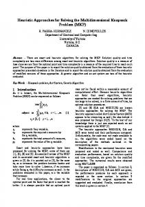
The distance graph corresponding to the (a) original, (b) minimal, (c) decoupled, and (d) fully assigned, versions of the example problem. 16 Ann’s FPC STN. . . . . . . . . . . . . . . . . . . . . . . . . . . . . 22 Ann’s DPC STN. . . . . . . . . . . . . . . . . . . . . . . . . . . . . 24 Ann’s PPC STN. . . . . . . . . . . . . . . . . . . . . . . . . . . . . 25 High-level overview of the MaSTP structure. . . . . . . . . . . . . . 32 Two alternative partitionings of an agent’s STP (a) into local vs. external components (b) and into shared vs. private components (c). 32 The temporal decoupling problem. . . . . . . . . . . . . . . . . . . . 34 Non-concurrent computation vs. P . . . . . . . . . . . . . . . . . . 52 Non-concurrent computation vs. A. . . . . . . . . . . . . . . . . . 53 Number of added fill edges vs. P . . . . . . . . . . . . . . . . . . . . 54 Relative (to centralized) number of added fill edges vs. P . . . . . . . 55 Applying the MaTDP algorithm to the example scheduling problem. 58 Nonconcurrent computation as A grows. . . . . . . . . . . . . . . . 65 Number of messages as A grows. . . . . . . . . . . . . . . . . . . . . 66 Nonconcurrent computation as N increases. . . . . . . . . . . . . . 66 Number of messages as N increases. . . . . . . . . . . . . . . . . . . 67 A disjunctive version of the running example problem. . . . . . . . . 74 The MaDTP is more general than alternative (single-agent) formulations. 82 The minimal, PPC STN distance graphs corresponding to the two feasible labellings of the problem in Table 3.1. . . . . . . . . . . . . 85 The minimal temporal network corresponding the example problem in Table 3.1. . . . . . . . . . . . . . . . . . . . . . . . . . . . . . . . 86 Local solution space vs. influence space. . . . . . . . . . . . . . . . . 98 Relative difference in computational effort using full vs. local decomposability. . . . . . . . . . . . . . . . . . . . . . . . . . . . . . . . . 99 Absolute difference in computational effort using full vs. local decomposability. . . . . . . . . . . . . . . . . . . . . . . . . . . . . . . . . 99 Runtime as the number of agents grows. . . . . . . . . . . . . . . . 101 Number of findSolution iterations as the number of agents grows. 101 Expected runtime of the MaDTP-TD vs. MaDTP-LD algorithms as coupling between agents increases. . . . . . . . . . . . . . . . . . . . 109

ix

3.11

3.12 3.13 3.14 3.15 3.16 4.1 4.2 4.3 4.4 4.5 4.6 4.7 4.8 4.9 4.10 4.11 4.12 4.13 4.14 4.15 5.1 5.2 5.3

Ratio of completeness of the output of the MaDTP-TD algorithm to the output of the MaDTP-LD algorithm as coupling between agents increases. . . . . . . . . . . . . . . . . . . . . . . . . . . . . . . . . . 111 Expected runtime of the MaDTP-TD vs. MaDTP-LD algorithms as number of agents increases. . . . . . . . . . . . . . . . . . . . . . . . 112 Ratio of completeness of the output of the MaDTP-TD algorithm to the output of the MaDTP-LD algorithm as number of agents increases.113 Expected runtime of the MaDTP-TD algorithm as number of agents increases. . . . . . . . . . . . . . . . . . . . . . . . . . . . . . . . . . 114 Expected runtime of Phase 1 of the MaDTP-TD algorithm as number of agents increases. . . . . . . . . . . . . . . . . . . . . . . . . . . . 115 Expected runtime of Phase 2 of the MaDTP-TD algorithm as number of agents increases. . . . . . . . . . . . . . . . . . . . . . . . . . . . 116 Logarithmic scale of the median number of conflicts, decisions, and seconds as agents handle additional activities. . . . . . . . . . . . . 141 Logarithmic scale of the expected number of conflicts, decisions, and seconds as agents handle additional activities. . . . . . . . . . . . . 142 Agents handling more constraints. . . . . . . . . . . . . . . . . . . . 143 Increasing temporal constraints precision. . . . . . . . . . . . . . . . 145 Increasing finite domain size. . . . . . . . . . . . . . . . . . . . . . . 147 Increasing the number of finite-domain variables. . . . . . . . . . . . 149 Finer granularity of temporal bounds. . . . . . . . . . . . . . . . . . 151 Partially-conditional temporal constraints. . . . . . . . . . . . . . . 153 Increasing the number of temporal disjunctions. . . . . . . . . . . . 156 The effects of HCT on solve time. . . . . . . . . . . . . . . . . . . . 158 The correlation between memory and solve time. . . . . . . . . . . . 159 The correlation between number of decisions and solve time. . . . . 160 The effects of HCT on the number of search decisions. . . . . . . . . 161 New HCT impact on solve time. . . . . . . . . . . . . . . . . . . . . 162 New HCT impact on number of decisions. . . . . . . . . . . . . . . 163 Total computational time of incremental algorithms. . . . . . . . . . 173 Ratio of decoupling update effort to least-commitment update effort as t increases. . . . . . . . . . . . . . . . . . . . . . . . . . . . . . . 175 Ratio of decoupling update effort to least-commitment update effort as N increases. . . . . . . . . . . . . . . . . . . . . . . . . . . . . . 176

x

LIST OF TABLES

Table 1.1 2.1 2.2 3.1 4.1 4.2 4.3 4.4 5.1

Overview of foundational and related approaches. . . . . . . . . . . 14 Summary of the running example problem. . . . . . . . . . . . . . . 19 The rigidity values of various approaches. . . . . . . . . . . . . . . . 70 Summary of the example MaDTP. . . . . . . . . . . . . . . . . . . . 76 Hybrid constraints related to the duration of Ann’s recreation activity.119 Example of hybrid constraint tightening for the hybrid constraints related to Ann’s recreational activity. . . . . . . . . . . . . . . . . . 130 Possible decouplings of the conditional minimum duration constraint. 135 Example of problem generator hybrid constraints. . . . . . . . . . . 138 The frequency of broken decouplings. . . . . . . . . . . . . . . . . . 174

xi

LIST OF ALGORITHMS

Algorithm 2.1 2.2 2.3 2.4 2.5 2.6 2.7 2.8 2.9 2.10 2.11 3.1 3.2 3.3 4.1 4.2

Floyd-Warshall . . . . . . . . . . . . . . . . . . . . . . . . . . . . . 22 Triangulate . . . . . . . . . . . . . . . . . . . . . . . . . . . . . . . 23 Directed Path Consistency (DPC) . . . . . . . . . . . . . . . . . . . 24 Planken’s Partial Path Consistency (P3 C) . . . . . . . . . . . . . . 25 Triangulating Directed Path Consistency (4DPC) . . . . . . . . . . 40 Triangulating Partial Path Consistency (4PPC) . . . . . . . . . . . 41 Partially Centralized Partial Path Consistency (PC4PPC) . . . . . 42 Distributed Directed Path Consistency (D4DPC) . . . . . . . . . . 45 Distributed Partial Path Consistency (D4PPC) . . . . . . . . . . . 48 Multiagent Temporal Decoupling Problem (MaTDP) . . . . . . . . 57 Multiagent Temporal Decoupling Relaxation (MaTDR) . . . . . . . 62 Multiagent Disjunctive Temporal Problem Local Decomposability (MaDTP-LD) . . . . . . . . . . . . . . . . . . . . . . . . . . . . . . 95 Multiagent Disjunctive Temporal Decoupling Algorithm (MaDTP-TD)106 Shared DTP Decoupling Procedure . . . . . . . . . . . . . . . . . . 107 Hybrid Constraint Tightening Algorithm . . . . . . . . . . . . . . . 129 Revised Hybrid Constraint Tightening Algorithm . . . . . . . . . . 161

xii

ABSTRACT

This research focuses on building foundational algorithms for scheduling agents that assist people in managing their activities in environments in which tempo and complexity outstrip people’s cognitive capacity. The critical challenge is that, as individuals decide how to act on their scheduling goals, scheduling agents should answer queries regarding the events in their interacting schedules while respecting individual privacy and autonomy to the extent possible. I formally define both the Multiagent Simple Temporal Problem (MaSTP) and Multiagent Disjunctive Temporal Problem (MaDTP) for naturally capturing and reasoning over the distributed but interconnected scheduling problems of multiple individuals. My hypothesis is that combining a bottom-up approach — where an agent externalizes constraints that compactly summarize how its local subproblem affects other agents’ subproblems, with a top-down approach — where an agent proactively constructs and internalizes new local constraints that decouple its subproblem from others’, will lead to effective solution techniques. I confirm that my hypothesized approach leads to distributed algorithms that calculate summaries of the joint solution space for multiagent scheduling problems, without centralizing or otherwise redistributing the problems. In both the MaSTP and MaDTP domains, the distributed algorithms permit concurrent execution for significant speedup over current art, and also increase the level of privacy and independence in individual agent reasoning. These algorithms are most advantageous for problems where interactions between the agents are sparse compared to the complexity of agents’ individual scheduling problems. Moreover, despite the combinatorially-large and unwieldy nature of the MaDTP solution space, I show that agents can use influence spaces, which compactly capture the impact of agents’ interacting schedules, to tractably converge on distributed summaries of the joint solution space. Finally, I apply the same basic principle to the Hybrid Scheduling Problem, which combines constraint-based scheduling with a rudimentary level of planning, and show that my Hybrid Constraint Tightening precompilation algorithm can improve the propagation of information between planning and scheduling subproblems, leading to significant search space pruning and execution time reduction. xiii

CHAPTER 1

Introduction

1.1

Motivation

Computational scheduling agents can assist people in managing and coordinating their activities in environments in which tempo, a limited (local) view of the overall problem, and complexity can outstrip people’s cognitive capacity. Often, the schedules of multiple agents interact, which yields the additional responsibility for an agent to coordinate its schedule with the schedules of other agents. However, each individual agent, or its user, may have strategic interests (privacy, autonomy, etc.) that prevent simply centralizing or redistributing the problem. In this setting, a scheduling agent is responsible for autonomously managing the scheduling constraints as specified by its user. As a concrete example, consider Ann, who faces the cognitively demanding challenge of processing the implications of the complex constraints of her busy schedule. A further challenge for Ann is that her schedule is interdependent with the schedules of her colleagues, family, and friends with whom she interacts. At the same time, Ann would still prefer the independence to make her own scheduling decisions and to keep her consultations with her doctor Chris from impinging on recreational activities with her friend Bill, thus using privacy to maintain a healthy separation between her personal, professional, and social lives. One of the challenges here is that, while Ann may lack sufficient time to realize and reason through the implications of scheduling decisions, she may still desire to exercise the autonomy that comes with making her own decisions. One way an agent can support this is to provide answers to queries Ann asks regarding the possible timings and relationships between events, rather than dictating particular scheduling decisions. These types of queries can help Ann to determine not only if one of her scheduling goals is achievable, but also, once this goal is expressed, to understand the implications it could have on other parts of her schedule. This allows Ann to decide if 1

there are unintended or undesirable consequences to a particular scheduling decision that may invalidate her original intent. It also provides Ann with possible courses of action to be able to achieve her long-term scheduling goals. This back-and-forth with her agent can also assist Ann with the more cognitively demanding task of deciding how to deal with contingent events, a task that can become especially strenuous in highly dynamic environments. A scheduling agent must then be equipped to handle the many kinds of scheduling queries that would help a user naturally evaluate his or her scheduling goals. There might be queries regarding when an activity can be executed, such as “Can I start this activity now, or alternatively, at time X?” or more generally, “When can I start this activity?” There could be queries about relationships between various events or activities, such as “How long should this activity take?” or “How much time will I have between these two activities?” A user may also wish to evaluate a possible scheduling goal, and thus pose queries that are based on a speculative or prospective constraint. Examples of these kinds of queries might include “If I start activity X now, how much time will I have for activity Y later?” or “If I want to give myself time to perform activity X in the afternoon, which activities could I start now that will allow me to do so?” Finally, for the answers to such queries to be meaningful, agents must be able to update their advice in the presence of new, dynamically-introduced constraints. These queries reflect a wide range of motives and goals, but, at their core, there is a fundamentally common structure to each of them: “provide me the bounds on intervals of possible times between two events (or one event and its possible clock times), given a (possibly null) condition that I may wish to achieve.” A scheduling agent, then, can efficiently support such queries (and provide reliable advice to its user) by preprocessing which spaces of schedules are feasible, and which are not. Further, a scheduling agent that presents a user with advice based on spaces of solutions is more robust than one that simply dictates a single schedule, which may be brittle to the dynamics involved in the problem (due to new constraints from its user, additional planning by other agents, or other dynamically arriving constraints). Finally, an agent should be prepared to efficiently update the space of solutions in response to a scheduling decision by its user or to other scheduling disturbances that arise. A challenge for agents that are maintaining spaces of schedules is that the introduction of a new constraint by one agent may impact many other agents, requiring that agents work together to maintain spaces of joint schedules. In many environments, updates to a schedule may occur quite frequently. For example, as Ann executes her

2

daily schedule, her agent should ensure ongoing consistent advice by incorporating the events and activities that Ann executes as new dynamically-arriving constraints. However, compared local reasoning, communication between agents tends to be significantly slower, intermittent, or altogether uncertain, which can inhibit agents from providing unilateral, time-critical, and coordinated scheduling assistance. Fortunately, agents can instead trade some of the completeness of the joint solution space in favor of decreased reliance on communication by way of a temporal decoupling, which is composed of independent sets of locally consistent spaces of schedules that, when combined, form a space of consistent joint schedules (Hunsberger, 2002). This allows an agent to make time-critical scheduling decisions and respond to rapidly occurring scheduling disturbances in an independent, efficient manner. Continuing my ongoing example, Chris’ schedule may be full of many medical consultations, the execution of each of which could incrementally affect Chris’ future availability and hence should be communicated so that, e.g., Ann’s agent can adjust her schedule accordingly. However, if network connectivity is intermittent or slow, such messages to Ann’s agent could get delayed, or worse, never be delivered at all, leading Ann’s agent to possibly give scheduling advice that is stale or incorrect. If, instead, Chris’ and Ann’s agents can initially agree on an a prescription hand-off time, then no further communication is needed unless or until one of the agents determines it cannot uphold this commitment locally. A temporal decoupling ensures that Chris’ agent can flexibly adapt to changes in Chris’ schedule without impacting Ann’s schedule at all, allowing Ann’s agent to independently manage her schedule as well. While throughout this section I have used an agent that acts as a scheduling assistant of human users to motivate my work, there are many other applications of the ideas explored and developed in this dissertation. These include coordinating embodied agents in disaster relief, military, or Mars rover operations; the automated scheduling of integrated manufacturing, transportation, or health care systems; and the distributed allocation of continuous resources, such as energy. While each of these applications may balance efficient decision-making support with relative costs and problems of communication differently, all have in common agents with a desire or need to maintain some level of independence so as to uphold the strategic benefits of distributed, independent schedule management. This is at the core of the problem description presented next.

3

1.2

Problem Statement

The overarching challenge that this thesis addresses is that of scheduling agents efficiently working together to compute consistent summaries of joint schedules, despite distributed information, implicit constraints, costs in sharing information among agents (e.g., delays, privacy, autonomy, etc.), and the possibility of new constraints dynamically arising. The pervasiveness of networked computational devices, coupled with naturally distributed problem representations and agents’ strategic desires, argue for agents that solve such scheduling problems using distributed algorithms and representations. The problem that this thesis addresses, then, is flexibly combining reasoning about interactions between agents’ schedules with more independent reasoning within an agents’s local schedules. Finding the right balance between agents that can render scheduling advice based on complete joint solution spaces and agents that can independently render sound advice is a challenge. A scheduling agent that provides complete scheduling advice keeps its user maximally informed and provides both maximal flexibility over scheduling decisions and maximal robustness in the midst of dynamic scheduling environments. On the other hand, a scheduling agent that is independent of others provides its user with maximal privacy and complete autonomy (within its local space of feasible schedules), while eliminating reliance on slow or intermittent communication between agents. These relative advantages and trade-offs argue for solution approaches that can flexibly trade between complete spaces of sound joint schedules and partial spaces of sound local schedules that agents can reason over independently. As Bill specifies his activities and constraints to his individual scheduling agent, he presumably assumes some level of privacy and personal control over his scheduling problem. At the same time, if Ann and Bill mutually agree to a constraint that relates activities from each of their respective scheduling problems, they have inherently lost privacy and unilateral control over some of their particular activities. Beyond what is already shared among agents due to agreed upon interagent constraints, a goal of my thesis is to maintain the maximum level of independence between agents’ problems possible, regardless of an agent’s motivation for desiring independence. Thus, throughout this thesis, I will assume that an agent is not permitted to reveal any more of its local subproblem to other agents beyond what is inherently revealed by mutually-known constraints. The result of this is that scheduling agents are permitted to share information over already mutually-known events and activities, but forbidden to reveal any local information that cannot be directly inferred from the shared

4

information. An additional challenge is that just because an agent’s activity is not directly constrained with another agent’s does not mean it cannot impact another agent; thus any solution approach must find a way to consistently capture such implicit constraints without growing the shared problem. Finally, the adoption of distributed scheduling agents is more likely if it represents a computational improvement over the current art. Thus, I require that all solution approaches for distributed scheduling agents produce speedup over known state-of-theart solution approaches, all of which currently execute in a centralized fashion. When interdependencies between agents are sparse compared to the complexity of agents’ local problems, there is hope for speeding solution algorithms over the current art in at least two ways. First, even centralized solution algorithms can exploit loosely-coupled problem structure by decomposing multiagent problems into largely independent subproblems and solving these subproblems separately and more efficiently using a divide-and-conquer strategy. Second, loose-coupling between agents’ problems affords opportunities for independent, concurrent agent reasoning, further speeding execution over single-agent, centralized approaches. Given that both of these potential sources of speedup rely on sparse relationships between problems, the amount of speedup will likely depend on the relative level of interagent coupling. Informally then, the problem this thesis solves is that of calculating a distributed summary of the joint solution space of multiagent scheduling problems without centralizing or otherwise redistributing the problem while achieving computational speedup over current art. I will restate this problem formally in Section 2.4 and Section 3.4 after I have more precisely defined novel constraint-based scheduling problem formulations.

1.3

Approach

The goal of this thesis is to solve multiagent, constraint-based scheduling problems that are naturally distributed, while promoting independent reasoning between agents’ problems. I will introduce multiagent, constraint-based problem formulations that compactly represent interacting schedules of multiple agents with n local problems, which leads to n subproblems, one for each of the n agents involved in the problem, and a set of external constraints that relate the activities of different agents. This representation explicitly captures loosely-coupled problem structure when it exists, thus avoiding the strategic costs typically associated with centralization (privacy, autonomy, etc.).

5

A distributed problem representation is maximally useful if there also exists an approach than can flexibly combine shared reasoning about interactions between agents’ schedules with local reasoning of individual agents about their local problems, without impeding the speed or quality of the overall solution approach. Here I discuss two complementary processes, an externalization process and internalization process, that exploit both the natural problem decomposition and also the availability of independently-executing agents to speed the solution process. Together these two processes help agents collectively understand not only how their schedules are intertwined, but also how to further disentangle them to further increase independent reasoning. Given the distributed nature of my approach, my algorithms will perform better as the opportunities for independent local reasoning grows, for example, as the sizes of, complexities of, and balance between agents’ local problems grow. Conversely, as the need for reasoning about interactions increases, for example as the number of external constraints between agents’ problems grows, the performance of my algorithms will suffer. Further, my algorithms are tunable to the degree to which new constraints are introduced. If many constraints are introduced over time, agents can invest the time to find the complete space of all joint schedules. Alternatively, if only very few constraints will be introduced, agents can sacrifice the completeness of the solution space for increased independent reasoning and improved computational runtimes. Finally, as the problems scale to include more agents, these tendencies will become more exaggerated, for example, emphasizing the value of distributed, independent reasoning for loosely-coupled problems, or alternatively, highlighting the de facto centralization of my approach for highly-coupled problems. 1.3.1

The Externalization Process

The main thrust behind the externalization process is that, in order to compute a distributed summary of the joint solution space, each agent must communicate the impact that its local problem has on other agents’ problems. The insight that I exploit throughout this thesis is that each agent can independently build a compact local constraint summary of this impact by abstracting away portions of its local problem that do not directly influence others, while simultaneously building new constraints that succinctly summarize how local constraints affect the shared problem in terms of mutually-known aspects of the problem. This avoids the privacy, communication, and autonomy costs of centralized approaches while exploiting the loosely-coupled structure between agents to achieve increased computational independence and speedup. 6

1.3.2

The Internalization Process

Agents should revise their distributed summary of the joint solution space as new constraints, which can render the solution space obsolete, arise. If such constraints arise frequently, or if interagent communication is especially slow or costly, an agent may lose its ability to provide sound advice efficiently. The main thrust behind the internalization process is to sacrifice a portion of the joint solution space so that each agent can independently and unilaterally reason over its own local solution space. The insight that I exploit is that agents can replace external constraints that relate the problems of two or more agents’ problems with new local (i.e., internal ) decoupling constraints that inherently satisfy the replaced external constraints. In contrast to previous centralized approaches, this process increases the amount of independent, private, and unilateral reasoning that an agent can perform. 1.3.3

An Integrated Approach

The externalization and internalization processes can be combined in a complementary way that balances the shared and local reasoning of agents and improves overall efficiency. The local constraint summarization process helps an agent understand how its problem is entangled with others’, thus informing and improving the disentangling, decoupling process. Likewise, by decoupling their interacting spaces of schedules, agents reduce the impact their local schedules have on one another, reducing the need for further coordination. Moreover, these two approaches represent a natural trade-off between increased independent reasoning on one hand, and increased joint flexibility on the other, which is useful since each application may require a different trade-off point depending on its specific goals and environments. 1.3.4

Evaluation

I analytically evaluate the runtime properties and correctness (soundness and completeness) of all algorithms that implement my approach. I also empirically compare the runtime performance my algorithms against the current art, which to this point has been exclusively centralized in nature, to evaluate whether my algorithms achieve computational speedup. To test how my algorithms perform as the demand for reasoning about interactions between agents’ schedules versus reasoning about local schedules varies, I hold the number and size of agent problems constant while varying the number of external constraints between problems. As the number of external constraints grows, so does the size of the problem that requires shared reasoning, while

7

the portion of the problem that each agent can reason over independently shrinks. I also test how my the performance of my algorithms responds as the number of agents increases. I report metrics that capture runtime and communication costs. To evaluate the completeness of the temporal decoupling that my algorithms calculate, I adopt, and as necessary adapt, existing metrics of flexibility that attempt to measure the portion of the complete joint solution space that is sacrificed in favor of increased independence between agents’ problems.

1.4

Contributions

Current approaches in multiagent scheduling (Dechter et al., 1991; Hunsberger, 2002; Xu & Choueiry, 2003; Planken et al., 2008b, 2010a) either require an additional coordination mechanism, such as a coordinator that calculates a (set of) solution schedule(s) for all or simply ignore relationships between subproblems altogether. The computational, communication, and privacy costs associated with centralization may be unacceptable in multiagent scheduling applications, where users specify problems in a distributed fashion and expect some degree of privacy and autonomy. Further, not only does the complexity of representing and calculating the space of feasible joint schedules grow with each additional agent, but generating joint schedules for every eventuality that could arise can compromise the privacy and autonomy interests of individual scheduling agents and introduces significant computational overhead. The contributions of my thesis, which I highlight next, use distributed representations and approaches to to reduce the computational, communication, and privacy costs of current approaches. 1.4.1

Multiagent, Constraint-based Scheduling Formulations

A contribution of this thesis is the formal definition of multiagent problem formulations that can capture scheduling problems involving interrelated activities that belong to different agents. A multiagent problem formulation allows problems to be specified in a distributed manner, with each user specifying his or her activities and constraints directly to his or her agent, which leads to n subproblems, one for each of the n agents involved in the problem. Furthermore, agents can better preserve the privacy and autonomy of their user in a distributed setting. My problem formulation also augments the n agent subproblems with a set of external constraints that relate the activities of different agents. External constraints only exist when interactions between the activities of different agents exist. This 8

helps limit the scope of the mutually known and jointly represented aspects of the problem to only what is necessary so that, if relationships are limited and looselycoupled in nature, so will the underlying problem formulation. By eliminating the privacy and computational costs of centralized representations and techniques, this representation could benefit many current applications that use temporal networks to achieve multiagent coordination, such as disaster relief efforts, military operations, Mars rover missions, and health care operations (Laborie & Ghallab, 1995; Bresina et al., 2005; Castillo et al., 2006; Smith et al., 2007; Barbulescu et al., 2010). 1.4.2

Formal Analysis of Properties of a Multiagent Temporal Network

Temporal constraint networks have often been touted for their ability to represent spaces of feasible schedules as compact intervals of time that can be calculated efficiently (Dechter et al., 1991; Xu & Choueiry, 2003; Planken et al., 2008b). Another contribution of this thesis is to show that these advantages extend to distributed, multiagent temporal constraint networks, while also introducing a level of independence that agents can exploit in many ways. Properties of temporal networks such as minimality and decomposability have proven essential in representing the solution space for many centralized applications such as project scheduling (Cesta et al., 2002), medical informatics (Anselma et al., 2006), air traffic control (Buzing & Witteveen, 2004), and spacecraft control (Fukunaga et al., 1997). Not only do I show that these important properties extend to multiagent networks, but multiagent temporal networks can also afford increased independent reasoning. Unfortunately, multiagent scheduling applications wishing to exploit these properties have previously relied on either a centralized temporal network representation or, if independence was also needed, completely disjoint, separate agent networks. The multiagent applications that currently use centralized temporal networks may benefit from the increased compactness of and independent reasoning allowed by the multiagent temporal network. On the other hand, the multiagent applications that currently use separate, disjoint networks may benefit from directly establishing joint minimality and decomposability on the multiagent temporal network, while still performing independent reasoning over local problems. Minimality. A minimal temporal constraint network is one whose constraints represent the exact set of values (times) that can lead to solutions for each event or difference between two events. By using bounds over (sets of) time intervals, a minimal constraint is a compact, sound and complete representation of the space 9

of possible solutions for an event or constraint. This property allows an agent to exactly and efficiently respond to users’ queries. I demonstrate that minimality can be established for constraints in a multiagent temporal constraint network, and thus, for multiagent temporal constraint networks as a whole. Decomposability. A decomposable temporal constraint network is one where any locally consistent assignment to a subset of events (i.e., an assignment that respects all the constraints that exist among the subset of events) is guaranteed to be extensible to a sound, full solution. A trivial example of a decomposable network is a fully specified point solution. However, one of the advantages of a temporal network that is both minimal and decomposable is that decomposability provides a mechanism for efficiently returning a minimal network back to minimality after an update. This property also allows an agent to provide support for the compound nature of contingent queries. I demonstrate that establishing decomposable multiagent temporal constraint networks is always possible, but a representation that is both decomposable and minimal (i.e., least-commitment in the sense that it represents the complete space of solutions) typically results in a fully connected temporal network. Independence. I show that as problems become more loosely-coupled, agents’ local solution spaces become increasingly independent from one another. I prove that any dependence that does exist between agents’ problems can be channeled through the existing shared constraints between those agents’ problems. This in turn implies that the remainder of each agent’s local problem can be reasoned over independently, which increases concurrency, autonomy, and privacy while decreasing the need for communication and sequentialization between agents. 1.4.3

Algorithms for Calculating the Joint Solution Space of Multiagent Scheduling Problems

I develop algorithms that establish the joint solution space for constraint-based, multiagent scheduling representation. The algorithms implement my high-level idea of externalizing the constraints that summarize the impact that an agent’s local problem has on other agents’ problems. The algorithms also achieve significant speedup over current approaches, which grows as problems become more loosely-coupled. The key observation is that agents can execute largely independently by first focusing on abstracting away the non-externally constrained portions of their problems. In the case of more complex, disjunctive scheduling problems, I contribute a distributed 10

algorithm for calculating the joint space of solutions by borrowing the concept of an influence space from the decentralized planning community (Witwicki & Durfee, 2010). The idea behind an influence space is that many of an agent’s unique local schedules (plans) may impact other agents in exactly the same way, and thus agents can benefit from computing and exchanging only the constraints that uniquely impact other agents. The coordination of agents is a critical component within many multiagent systems applications including scheduling (e.g., Barbulescu et al. (2010)), planning (e.g., Witwicki & Durfee (2010)), resource and task allocation (e.g., Zlot & Stentz (2006)), among others. While my algorithms have been tailored to multiagent, constraintbased scheduling in particular, the high-level idea of summarizing the impact that one agent has on another by systematically abstracting away local problem details while capturing their implications is a high-level idea that could conceptually be applied in many multiagent coordination domains. My algorithms, which provide a summary of the space of all solutions, provide an alternative to modeling and reasoning over uncertainty (e.g., Vidal, 2000; Morris & Muscettola, 2005) and also flexible support for validating multiagent plan execution (e.g., Shah et al., 2009; Barbulescu et al., 2010). Finally, the ideas established here represent a novel contribution to the greater distributed constraint reasoning community, where my approach is unique in that it produces complete solution space with atypical guarantees of local privacy and autonomy. 1.4.4

Algorithms for Calculating Temporal Decouplings of Multiagent Scheduling Problems

The second set of algorithmic contributions that I make in my thesis is for computing temporal decouplings of multiagent scheduling problems. Unlike the algorithms for calculating the joint solution space, these algorithms are not based on existing centralized algorithms, but rather based on insights and properties of the algorithms mentioned in the previous subsection. The result is a novel incorporation of decoupling decisions into algorithms that summarize, exchange, and compute spaces of solutions and leads to significant speedup over current approaches. A temporal decoupling represents a sacrifice in the completeness of the space of feasible joint schedules for increased agent independence. While the relative importance of independence in agent reasoning vs. complete knowledge over the joint solution space is likely to be application dependent (e.g., depending on communication costs, level of dynamism, etc.), I contribute a comparison of the costs of these two approaches in terms of both 11

computational effort and flexibility. Flexibility metrics attempt to measure the portion of the joint solution space that is retained by a temporal decoupling. A distributed temporal decoupling algorithm is an important contribution over the current art (Hunsberger, 2002, 2003; Planken et al., 2010a) because it preserves privacy and exploits concurrent by decentralizing computation. In addition to providing another distributed technique for multiagent coordination, the beneficiaries of which were discussed in the previous section, I provide novel insights on how best to combine temporal decoupling with local constraint summarization to achieve greater efficiency, which leads to significant gains in algorithmic efficiency over Hunsberger (2002), even when this combination is executed in a centralized fashion. Additionally, temporal decoupling can be viewed as a proactive hedge against the uncertainty introduced by the presence of other agents, and thus contributes to the discussion of controllability and uncertainty (e.g., Vidal & Ghallab, 1996; Vidal, 2000). Conceptually, temporal decoupling algorithms can also be viewed as enforcing problem structure in a way that increases efficiency in representing and monitoring plan execution (e.g., Shah et al., 2009). Finally, my decoupling idea introduces a novel divide-first, conquer-second approach to increase independent reasoning in a way that can be applied in the distributed finite-domain constraint reasoning community. 1.4.5

Extension to Planning: Hybrid Constraint Tightening

Hybrid constraints capture the fact that often activity selection (e.g., deciding which recreational activity to perform), impacts how an activity is scheduled (e.g., each recreational activity may be differently affected by a weather forecast or hours of operation of local businesses). At some level, incorporating the power to select which activities are to be performed and how to perform them adds a rudimentary layer of planning to the multiagent scheduling problems I am investigating. Method. As a highlight of the generality of my basic approach, I contribute Hybrid Constraint Tightening (HCT), a preprocessing algorithm [Boerkoel and Durfee, 2008; 2009] that uses constraint summarization principles between an agent’s planning and scheduling subproblems rather than the scheduling subproblems of different agents. HCT reformulates hybrid constraints by lifting information from the structure of hybrid constraints. These reformulated constraints elucidate implied constraints between an agent’s planning and scheduling subproblems earlier in the search process, leading to significant search space pruning.

12

Empirical Evaluation. Despite the computational costs associated with applying the HCT preprocessing algorithm, HCT leads to orders of magnitude speedup when used in conjunction with off-the-shelf, state-of-the-art solvers, as compared to solving the same problem instance without applying HCT. However, the efficacy of HCT is dependent on the underlying structure of the constraints involved. I have systematically explored properties of hybrid constraints that influence HCTs efficacy, quantifying the influence empirically. Generally, the efficacy of HCT is increased as the size and complexity, especially of the finite-domain constraints involved in hybrid constraints, increases. Conversely, increased complexity of the temporal constraint component of hybrid constraints tends to mitigate HCT’s effectiveness. HCT will play a critical role in extending multiagent scheduling to incorporate rudimentary levels of planning. Planning and scheduling, while interrelated (Myers & Smith, 1999; Garrido & Barber, 2001; Halsey et al., 2004), are often treated as separate subproblems (e.g., McVey et al. (1997)). Thus, hybrid scheduling problems represent a way to bridge planning and scheduling, while HCT, then, contributes an understanding on how to improve reasoning between these two subproblems. Simply by reformulating hybrid constraints in a way that summarizes the impact one subproblem has on another, I can improve the efficiency of existing solvers. My contributions empirically demonstrate that applications that ignore the interplay between scheduling and planning do so at their own peril. As discussed in Section 4.3.3, HCT can be viewed as taking a step towards, to borrow a phrase from Smith et al. (2000), “bridging the gap between planning and scheduling”.

1.5

Overview

The logical flow of the rest of this thesis is as follows. Chapter 2 — The Multiagent Simple Temporal Problem, flows into Chapter 3 — The Multiagent Disjunctive Temporal Problem, which adds the possibility of representing multiagent disjunctive scheduling problems. Then, in addition to scheduling disjunction, I add the ability to select which activities are to be scheduled using the Hybrid Scheduling Problem in Chapter 4 — Hybrid Constraint Tightening. Chapter 5 concludes with a discussion about contributions and future research directions. The structure of my thesis presentation is atypical in that the background and related work are divided among each of the chapters, taking advantage of the fact that each chapter conceptually builds on the previous one in terms of problem complexity. There is uniformity across the structure of each chapter: a brief introduction section

13

is followed by a section to introduce foundational background work and then a section discussing related approaches. These sections are, in turn, followed by sections that describe my approach, including one to describe the new problem formulation (when one is needed), and sections that describe the implementations and evaluations of the approaches discussed in Section 1.3. The hope is comprehension and readability is increased by introducing key concepts closer to where they are most useful to the reader. I will progressively introduce the foundational and related work that my work builds upon. I start by introducing the Simple Temporal Problem (STP), its properties, existing solution approaches, and related models, approaches, and applications in Chapter 2. Then, in Chapter 3, I introduce the Disjunctive Temporal Problem (DTP), which adds a layer of complexity to the STP by allowing the representation of disjunctive scheduling problems, as well as its constituent and related approaches. Finally, I introduce the Hybrid Scheduling Problem (HSP), which adds a rudimentary level of planning by relating constraint-based scheduling subproblems with the activity selection allowed by finite-domain constraint satisfaction problems. I summarize this progression of foundational and related approaches in Table 1.1. Chapter Chapter 2 The Multiagent Simple Temporal Problem Chapter 3 The Multiagent Disjunctive Temporal Problem

Background Section 2.2 Simple Temporal Problem; Simple Temporal Networks; Temporal Decoupling Problem Section 2.2 Disjunctive Temporal Problem; DTP Search

Chapter 4 Hybrid Constraint Tightening

Section 4.2 Constraint Satisfaction Problem; Hybrid Scheduling Problem

Related Approaches and Applications Section 2.3 Simple Temporal Problem with Uncertainty; Dist. Coordination of Mobile Agent Teams; Bucket-Elimination Algorithms Section 2.3 Fast Dist. Multiagent Plan Execution; Resource and Task Allocation Problems; Operations Research Section 4.3 DT PF D ; Dist. Finite-Domain Constraint Reasoning; Multiagent Planning

Table 1.1: Overview of foundational and related approaches.

14

CHAPTER 2

The Multiagent Simple Temporal Problem

2.1

Introduction

The Simple Temporal Problem (STP) formulation is capable of representing scheduling problems, along with their corresponding solution spaces, where if the order between pairs of activities matters, this order has been predetermined. As such, the STP acts as the core scheduling problem representation for (and flexible representation of scheduling solutions to) many interesting planning problems (Laborie & Ghallab, 1995; Bresina et al., 2005; Castillo et al., 2006; Smith et al., 2007; Barbulescu et al., 2010). Likewise, the Multiagent STP (MaSTP) is as a multiagent, distributed representation of scheduling problems and their solutions for multiagent and can be used for multiagent plan execution and monitoring. As an example of this type of problem, suppose Ann, her friend Bill, and her doctor Chris, have each selected a tentative morning agenda (from 8:00 AM to noon) and have each tasked a personal computational scheduling agent with maintaining schedules that can accomplish his/her agenda. Ann will have a 60 minute recreational activity (RA ) with Bill before spending 90 to 120 minutes performing a physical therapy regimen to help rehabilitate an injured knee (T RA ) (after receiving the prescription left by her doctor Chris); Bill will spend 60 minutes recreating (RB ) with Ann before spending 60 to 180 minutes at work (W B ); and finally, Chris will spend 90-120 minutes planning a physical therapy regimen (T P C ) for Ann and drop it off before giving a lecture (LC ) from 10:00 to 12:00. This example is displayed graphically as a distance graph (explained in Section 2.2.1) in Figure 2.1(a), with each event (e.g., the start time, ST , and end time, ET ) appearing as a vertex, and constraints appearing as weighted edges. One approach, displayed graphically in Figure 2.1(d), is for agents to simply select one joint schedule (an assignment of specific times to each event) from the set of 15

Chris

8: 00,12: 00

8: 00,12: 00

90,120

𝐶 𝑇𝑃𝑆𝑇

8: 00,12: 00

8: 00,12: 00

60,60

𝐴 𝑅𝑆𝑇

𝐶 𝑇𝑃𝐸𝑇

Ann

8: 00,12: 00 𝐵 𝑅𝑆𝑇

𝐴 𝑅𝐸𝑇

Bill

8: 00,12: 00

60,60

𝐵 𝑅𝐸𝑇

0,0 𝐿𝐶𝑆𝑇

120,120

10: 00,10: 00

𝐴 𝑇𝑅𝑆𝑇

𝐿𝐶𝐸𝑇

12: 00,12: 00

90,120

8: 00,12: 00

𝐵 𝑊𝑆𝑇

𝐴 𝑇𝑅𝐸𝑇

8: 00,12: 00

60,180

8: 00,12: 00

𝐵 𝑊𝐸𝑇

8: 00,12: 00

(a) Original Example MaSTP. 8: 00,8: 30

Chris

9: 30,10: 00

90,120

𝐶 𝑇𝑃𝑆𝑇

Ann

8: 00,9: 30

60,60

𝐴 𝑅𝑆𝑇

𝐶 𝑇𝑃𝐸𝑇

9: 00,10: 30 𝐴 𝑅𝐸𝑇

8: 00,9: 30 𝐵 𝑅𝑆𝑇

0,0

Bill

9: 00,10: 30

60,60

𝐵 𝑅𝐸𝑇

60,150 𝐿𝐶𝑆𝑇

120,120

10: 00,10: 00

𝐴 𝑇𝑅𝑆𝑇

𝐿𝐶𝐸𝑇

12: 00,12: 00

90,120

9: 00,10: 30

𝐵 𝑊𝑆𝑇

𝐴 𝑇𝑅𝐸𝑇

10: 30,12: 00

60,180

9: 00,11: 00

𝐵 𝑊𝐸𝑇

10: 00,12: 00

(b) Dispatchable (PPC) Version. 8: 00,8: 30 𝐶 𝑇𝑃𝑆𝑇

Chris

9: 30,10: 00

90,120

𝐶 𝑇𝑃𝐸𝑇

8: 45,8: 45 𝐴 𝑅𝑆𝑇

Ann 60,60

9: 45,9: 45

8: 45,8: 45

𝐴 𝑅𝐸𝑇

𝐵 𝑅𝑆𝑇

𝐴 𝑇𝑅𝐸𝑇

𝐵 𝑊𝑆𝑇

Bill

9: 45,9: 45

60,60

𝐵 𝑅𝐸𝑇

60,105 𝐿𝐶𝑆𝑇

120,120

10: 00,10: 00

8: 00

𝐿𝐶𝐸𝑇

12: 00,12: 00

Chris

9: 30

𝐴 𝑇𝑅𝑆𝑇

90,120

10: 00,10: 30

10: 30,12: 00

(c) Decoupled Version. Ann 9: 00

8: 00

60,135

9: 45,11: 00

8: 00

𝐵 𝑊𝐸𝑇

10: 45,12: 00

Bill

9: 00

𝐶 𝑇𝑃𝑆𝑇

𝐶 𝑇𝑃𝐸𝑇

𝐴 𝑅𝑆𝑇

𝐴 𝑅𝐸𝑇

𝐵 𝑅𝑆𝑇

𝐵 𝑅𝐸𝑇

𝐿𝐶𝑆𝑇

𝐿𝐶𝐸𝑇

𝐴 𝑇𝑅𝑆𝑇

𝐴 𝑇𝑅𝐸𝑇

𝐵 𝑊𝑆𝑇

𝐵 𝑊𝐸𝑇

10: 00

12: 00

9: 30

11: 00

9: 00

10: 00

(d) Fully Assigned Version. Figure 2.1:

The distance graph corresponding to the (a) original, (b) minimal, (c) decoupled, and (d) fully assigned, versions of the example problem.

16

possible solutions. In this case, each agent can provide exact times when queried about possible timings and relationships between events, and do so confident that this advice will be independent of (and consistent with) the advice delivered by other agents. However, this also leads to agents offering very brittle advice, where, as soon as a new constraint arrives (e.g., Chris’ bus arrives late by even a single minute), this exact, joint solution may no longer be valid. This, in turn, can require agents to regenerate a new solution every time a new constraint arrives, unless that new constraint happens to be consistent with the currently selected schedule. A second approach for solving this problem is to represent the set of all possible joint schedules that satisfy the constraints, as displayed in Figure 2.1(b). This leads to advice that is much more robust to disturbances and accommodating to new constraints. In this approach, if a new constraint arrives (e.g., Chris’ bus is late), the agents can easily recover by simply eliminating inconsistent joint schedules from consideration. However, doing so may still require communication (e.g., Chris’ agent should communicate that her late start will impact when Ann can start therapy). The need for communication may continue (e.g., until Chris actually completes the prescription, Ann cannot start the therapy regimen), otherwise agents risk making inconsistent, concurrent decisions. For example, if both Ann’s and Bill’s agent report that recreation can start any time from 8:00 to 9:30 (all allowable times), but Ann decides to start at 8:00 while Bill decides to start at 9:00, the agents will have inadvertently given inaccurate (uncoordinated) advice, since Ann and Bill must start the recreation activity together. There is also a third approach that attempts to balance the resiliency of Figure 2.1(b) with the independence of Figure 2.1(d). Agents can find and maintain a temporal decoupling, which is composed of independent sets of locally consistent schedules that, when combined, form a set of consistent joint schedules (Hunsberger, 2002). An example of a temporal decoupling is displayed in Figure 2.1(c), where, for example, Chris’ agent has agreed to prescribe the therapy regimen by 10:00 and Ann’s agent has agreed to wait to begin performing it until after 10:00. Then, not only will the agents’ advice be independent of other agents’, but it also provides agents with some resiliency to new constraints and offers users some flexibility and autonomy in making their own scheduling decisions. Now when Chris’ bus is late by a minute, Chris’ agent can absorb this new constraint by independently updating its local set of schedules, without requiring any communication with any other agent. The advantage of this approach is that once agents establish a temporal decoupling, there is no need for further communication unless (or until) a new (group of) constraint(s) render

17

the chosen decoupling inconsistent. It is only if and when a temporal decoupling does become inconsistent (e.g., Chris’ bus is more than a half hour late, violating her commitment to finish the prescription by 10:00) that agents must calculate a new temporal decoupling (perhaps establishing a new hand-off deadline of 10:15), and then once again independently react to newly-arriving constraints, repeating the process as necessary. Unfortunately, current solution algorithms (Dechter et al., 1991; Hunsberger, 2002; Xu & Choueiry, 2003; Planken et al., 2008b, 2010a) require centralizing the problem representation at some coordinator who calculates a (set of) solution schedule(s) for all. The computation, communication, and privacy costs associated with centralization may be unacceptable in multiagent planning and scheduling applications, such as military, health care, or disaster relief, where users specify problems to agents in a distributed fashion, and agents are expected to provide private, unilateral, time-critical, and coordinated scheduling assistance, to the extent possible. In this chapter, I contribute new, distributed algorithms for finding both the complete joint solution space and temporal decouplings of the MaSTP. I prove the correctness and runtime properties of each these algorithms, including the level of independent, private reasoning that distributed algorithms can achieve. I also empirically compare the approaches, both with each other, to show the trade-offs in completeness vs. independence in reasoning, and with state-of-the-art centralized approaches, to show significant speedup over these approaches.

2.2

Background

In this section, I provide definitions necessary for understanding my contributions, using and extending terminology from the literature. 2.2.1

Simple Temporal Problem

As defined by Dechter et al. (1991), the Simple Temporal Problem (STP), S = hX, Ci, consists of a set of timepoint variables, X, and a set of temporal difference constraints, C. Each timepoint variable represents an event and has a continuous domain of values (e.g., clock times) that can be expressed as a constraint relative to a special zero timepoint variable, z ∈ V , which represents the start of time. Each temporal difference constraint cij is of the form xj − xi ≤ bij , where xi and xj are distinct timepoints, and bij ∈ R is a real number bound on the difference between xj and xi . Often, as notational convenience, two constraints, cij and cji , of the form 18

bji ≤ xj − xi ≤ bij are represented as a single constraint of the form xj − xi ∈ [−bji , bij ]. A schedule is an assignment of specific time values to timepoint variables. An STP is consistent if it has at least one solution, which is a schedule that respects all constraints.

Ann

Bill

Chris

Availability A − z ∈ [480, 720] RST A − z ∈ [480, 720] RET A − z ∈ [480, 720] T RST A − z ∈ [480, 720] T RET B − z ∈ [480, 720] RST B − z ∈ [480, 720] RET B − z ∈ [480, 720] WST B − z ∈ [480, 720] WET C − z ∈ [480, 720] T PST C − z ∈ [480, 720] T PET LC ST − z ∈ [600, 600] LC ET − z ∈ [720, 720]

Duration A RET

−

A RST

∈ [60, 60]

A − T RA ∈ [90, 120] T RET ST

B − RB ∈ [60, 60] RET ST B WET

−

B WST

Ordering A − T RA ≤ 0 RET ST

External A RST

B ∈ [0, 0] − RST

C − T RA ≤ 0 T PET ST

B − WB ≤ 0 RET ST

A − RB ∈ [0, 0] RST ST

C − LC ≤ 0 T PET ST

C − T RA ≤ 0 T PET ST

∈ [60, 180]

C − T P C ∈ [90, 120] T PET ST C LC ET − LST ∈ [120, 120]

Table 2.1: Summary of the running example problem. In Table 2.1, I formalize the running example with specific constraints. Each activity has two timepoint variables representing its start time (ST ) and end time (ET ), respectively. In this example, all activities are to be scheduled in the morning (8:00-12:00), and so are constrained (Availability column) to take place within 480 and 720 of the zero timepoint z, which in this case is the start of day (midnight). Duration constraints are specified with bounds over the difference between an activity’s end time and start time, whereas Ordering constraints dictate the order in which an agent’s activities must take place with respect to each other. Finally, while a formal introduction of external constraints is deferred until later (Section 2.4), the last column represents constraints that span the subproblems of different agents. Figure 2.1 (d) illustrates a schedule that represents a solution to this particular problem. 2.2.2

Simple Temporal Network

To exploit extant graphical algorithms (e.g., shortest path algorithms) and efficiently reason over the constraints of an STP, each STP is associated with a Simple Temporal Network (STN), which can be represented by a weighted, directed graph, G = hV, Ei, called a distance graph (Dechter & Pearl, 1987). The set of vertices V contains a vertex vi for each timepoint variable xi ∈ X, and E is a set of directed edges, where, for each constraint cij of the form xj − xi ≤ bij , a directed edge, eij from vi to vj is constructed with an initial weight wij = bij . As a graphical short-hand, each

19

edge from vi to vj is assumed to be bi-directional, capturing both edge weights with a single interval label, [−wji , wij ], where vj − vi ∈ [−wji , wij ] and wij or wji is initialized to ∞ if there exists no corresponding constraint cij ∈ C or cji ∈ C, respectively. An STP is consistent if and only if there exist no negative cycles in the corresponding STN distance graph. The reference edge, ezi , of a timepoint vi is the edge between vi and the zero timepoint z. As another short-hand, each reference edge ezi is represented graphically as a self-loop on vi . This self-loop representation underscores how a reference edge eiz can be thought of as a unary constraint that implicitly defines vi ’s domain, where wzi and wiz represent the earliest and latest times that can be assigned to vi , respectively. In this thesis, I will assume that z is always included in V and that, during the construction of G, a reference edge ezi is added from z to every other timepoint variable vi ∈ V . The graphical STN representation of the example STP given in Table 2.1 is A A displayed in Figure 2.1 (a). For example, the duration constraint T RET − T RST ∈ A A [90, 120] is represented graphically with a directed edge from T RST to T RET with B B label [90, 120]. Notice that the label on the edge from RET to WST has an infinite upper bound, since while there is a constraint that dictates that Bill must start work after he ends recreation, there is no corresponding constraint dictating how soon after he ends recreation that this must occur. Finally, the constraint LC ST − z ∈ [600, 600] is C translated to a unary loop on LST , with a label of [10:00,10:00], which represents that Chris is constrained to start the lecture at exactly 600 minutes after midnight (or at exactly 10:00 AM). Throughout this thesis, I use both STP and STN notation. The distinction is that STP notation captures properties of the original problem, such as which pair of variables are constrained with which bounds, whereas STN notation is a convenient, graphical representation of STP problems that agents can algorithmically manipulate in order to find solutions by, for example, capturing implied constraints as new or tightened edges in the graph. 2.2.3

Useful Simple Temporal Network Properties

Temporal networks that are minimal and decomposable provide an efficient representation of an STP’s solution space that can be useful to advice-wielding scheduling agents. Minimality. A minimal constraint cij is one whose interval bounds, wij and wji , exactly specify the set of all values for the difference vj − vi ∈ [−wji , wij ] that are part 20

of any solution. A temporal network is minimal if and only if all of its constraints are minimal. A minimal network is a representation of the solution space of an STP. For example, Figure 2.1 (b) is a minimal STN, whereas (a) is not, since it would allow Ann to start recreation at, say, 9:31 and (c) is also not since it does not allow Ann to start at 9:30. More practically, a scheduling agent can use a minimal representation to exactly and efficiently suggest scheduling possibilities to users without overlooking options or suggesting options that will not work. Decomposability. Decomposability facilitates the maintenance of minimality by capturing constraints that, if satisfied, will lead to global solutions. A temporal network is decomposable if any assignment of values to a subset of timepoint variables that is locally consistent (satisfies all constraints involving only those variables) can be extended to a solution (Dechter et al., 1991). For example, Figure 2.1 (d) is trivially A decomposable, while (b) is not, since, for instance, the assignment RET = 10:30 and A T RET = 10:30, while self-consistent (because there are no constraints directly between these two variables), cannot be extended to a solution. A scheduling agent can use a decomposable temporal network to directly propagate any newly-arriving constraint(s) to any other area of the network in a single-step, backtrack-free manner. In sum, an STP that is both minimal and decomposable represents the entire set of solutions by establishing the tightest bounds on timepoint variables such that: (1) no solutions are eliminated and (2) any self-consistent assignment of a specific time to a subset of timepoint variables that respects these bounds can be extended to a solution in a backtrack-free, efficient manner. 2.2.4

Simple Temporal Problem Consistency Algorithms

In this subsection, I highlight various existing algorithms that each help establish the STN solution properties introduced in the previous subsection. Full-Path Consistency. Full-Path Consistency (FPC) works by establishing the minimality and decomposability of an STP instance in O (|V |3 ) by applying an all-pairs-shortest-path algorithm, such as Floyd-Warshall (1962) to its STN, resulting in a fully-connected distance graph. The algorithm, presented as Algorithm 2.1, finds the tightest possible path between every pair of timepoints, vi and vj , in the fully-connected distance graph, where ∀i, j, k, wij ≤ wik + wkj . The resulting graph is then checked for consistency by validating that there are no negative cycles, that is, ∀i 6= j, ensuring that wij + wji ≥ 0 (Dechter et al., 1991). An example of the 21

𝐴 𝑇𝑅𝑆𝑇

90,120

9: 00,10: 30

Algorithm 2.1 Floyd-Warshall Input: A fully-connected distance graph G = hV, Ei Output: A FPC distance graph G or inconsistent 1: for k = 1 . . . n do 2: for i = 1 . . . n do 3: for j = 1 . . . n do 4: wij ← min(wij , wik + wkj ) 5: if wij + wji < 0 then 6: return inconsistent 7: end if 8: end for 9: end for 10: end for 11: return G

10: 30,12: 00

Ann

8: 00,9: 30

9: 00,10: 30

60,60

𝐴 𝑅𝑆𝑇

[60,150] 𝐴 𝑇𝑅𝑆𝑇

𝐴 𝑇𝑅𝐸𝑇

𝐴 𝑅𝐸𝑇

[90,180] 90,120

9: 00,10: 30

𝐴 𝑇𝑅𝐸𝑇

10: 30,12: 00

Figure 2.2: Ann’s FPC STN.

FPC version of Ann’s STP subproblem is presented in Figure 2.2. Note that an agent using an FPC representation can provide exact bounds over the values that will lead to solutions for any pair of variables, regardless of whether or not a corresponding constraint was present in the original STP formulation. Graph Triangulation The next two forms of consistency require a triangulated (also called chordal) distance graph. A triangulated graph is one whose largest nonbisected cycle is a triangle (of length three). Conceptually, a graph is triangulated by the process of considering vertices and their adjacent edges, one-by-one, adding edges between neighbors of the vertex if no edge previously existed, and then eliminating that vertex from further consideration, until all vertices are eliminated. The basic graph triangulation algorithm is presented as Algorithm 2.2. The set of edges that are added during this process are called fill edges and the order in which timepoints are eliminated from consideration is referred to as an elimination order , o. The quantity ωo∗ is the induced graph width of the distance graph relative to o, and is defined as the maximum, over all vk , of the size of vk ’s set of not-yet-eliminated neighbors at the time of its elimination. Elimination orders are often chosen to attempt to find a minimal triangulation, that is to attempt to minimize the total number of fill edges. While, generally speaking, finding the minimum triangulation of a graph is an NP-complete problem, heuristics such as the minimum degree (selecting the vertex with fewest edges) and minimum fill (selecting the vertex that adds fewest fill edges) are used to efficiently

22

Algorithm 2.2 Triangulate Input: A distance graph G = hV, Ei; and elimination order o = (v1 , v2 , . . . , vn−1 , vn ) Output: A triangulated distance graph G 1: for k = 1 . . . n do 2: for all i, j < k s.t. eik , ejk ∈ E do 3: E ← E ∪ {eij } 4: end for 5: end for 6: return G

find elimination orders that approximate the minimum triangulation (Kjaerulff, 1990). Figure 2.3 shows a triangulated version of Ann’s distance graph where timepoints are A A A A eliminated in order o = (T RET , RET , RST , T RST ). Directional Path Consistency. An alternative to FPC for checking STP consistency is to establish Directional Path Consistency (DPC) on its distance graph (Dechter et al., 1991). The DPC algorithm, presented as Algorithm 2.3, takes a triangulated graph and corresponding elimination order, o, as input and then traverses each timepoint, vk , in elimination order o, tightening edges between each pair of neighboring timepoints, vi , vj , (each connected to vk via edges eij and ejk respectively) that appear after vk in order o, using the rule wij ← min(wij , wik + wkj ). The complexity of DPC is O (|V | · ωo∗2 ), but instead of establishing minimality, it establishes the property that a solution can be recovered from the DPC distance graph in a backtrack-free manner if variables are assigned in reverse elimination order. An example of a DPC version of A A A A Ann’s problem (using elimination order o = (T RET , RET , RST , T RST )) is presented in Figure 2.3. Basically, establishing DPC is sufficient for a scheduling agent that will need to give advice only with respect to a single-variable (the last one to be eliminated). Partial Path Consistency. Partial Path Consistency (PPC) (Bliek & SamHaroud, 1999) is sufficient for establishing minimality on an STP instance by calculating the tightest possible path for only the subset of edges that exist within a triangulated distance graph. An example is Xu and Choueiry’s algorithm 4STP (2003), which processes and updates a queue of all potentially inconsistent triangles (4) from the triangulated graph. Alternatively, in their algorithm P3 C, Planken et al. (2008b) sweep through these triangles in a systematic order, resulting in an improved expected runtime. The P3 C algorithm, which executes the DPC algorithm as a first phase also 23

Algorithm 2.3 Directed Path Consistency (DPC) Input: A triangulated temporal network G = hV, Ei and corresponding elimination order o = (v1 , v2 , . . . , vn−1 , vn ) Output: A DPC distance graph G or inconsistent 1: for k = 1 . . . n do 2: for all i < k s.t. eik ∈ E do 3: for all j < i s.t. ejk ∈ E do 4: wij ← min(wij , wik + wkj ) 5: wji ← min(wji , wjk + wki ) 6: if wij + wji < 0 then 7: return inconsistent 8: end if 9: end for 10: end for 11: end for 12: return G

8: 00,12: 00

Ann

8: 00,12: 00

60,60

𝐴 𝑅𝑆𝑇

𝐴 𝑅𝐸𝑇

[60, ∞ 𝐴 𝑇𝑅𝑆𝑇

90,120

9: 00,10: 30

𝐴 𝑇𝑅𝐸𝑇

8: 00,12: 00

Figure 2.3: Ann’s DPC STN.

8: 00,9: 30

Ann 60,60

9: 00,10: 30

executes a backwards traversal of the DPC algorithm as a second phase, where edge 𝐴 𝐴 𝑅𝑆𝑇 𝑅𝐸𝑇 weights are updated in reverse elimination order and thus achieves the same complexity, [60,150] O (|V | · ωo∗2 ), as the DPC algorithm. By exploiting sparse network topology, PPCbased algorithms may establish minimality much faster than FPC algorithms in 𝐴 𝐴 𝑇𝑅𝑆𝑇 𝑇𝑅𝐸𝑇 practice (O (|V | · ωo∗2 ) ⊆ O (|V |3 )) (Xu & Choueiry, 2003; Planken et al., 2008b). The 90,120 PPC representation of Ann’s subproblem is displayed in Figure 2.4. 9: 00,10: 30 10: 30,12: 00 PPC networks only approximate full decomposability, where assignments to subsets of variables are guaranteed extensible to a full solution only when the variables belong to the same clique in the triangulated network. However solutions can still be recovered in a backtrack free manner by either requiring constraint propagation between each subsequent variable assignment or by assigning variables in any reverse simplicial 9: 00,10: 30 8: 00,9: 30 elimination order — any elimination order of variables that would yield the same 60,60 𝐴 (Planken et al., 2008b). 𝐴 triangulated network (that is, introduce no new fill edges) An 𝑅𝑆𝑇 𝑅𝐸𝑇 agent using a PPC representation can offer advice over any pair of variables that were [60,150] (and those subsequently [90,180] originally related via a constraint in the original formulation added as fill edges). While unlike FPC temporal networks, an agent using𝐴a PPC 𝐴 𝑇𝑅𝑆𝑇 𝑇𝑅𝐸𝑇 network cannot answer queries regarding arbitrary pairs of variables 90,120 (i.e., those not related via a constraint in the original specification), the sparser PPC structure will 9: 00,10: 30 10: 30,12: 00 have important benefits for agents’ independent and private reasoning.

Ann

24

𝐴 𝑇𝑅𝑆𝑇

90,120

9: 00,10: 30

Algorithm 2.4 Planken’s Partial Path Consistency (P3 C)

2.2.5

8: 00,12: 00

Ann

8: 00,9: 30

Input: A triangulated temporal network G = hV, Ei and an elimination order o = (v1 , v2 , . . . , vn−1 , vn ) Output: A triangulated, PPC distance graph G or inconsistent 1: DPC(G, o) 2: return inconsistent if DPC did 3: for k = n . . . 1 do 4: for all i, j > k s.t. eik , ejk ∈ E do 5: wik ← min(wik , wij + wjk ) 6: wkj ← min(wkj , wki + wij ) 7: end for 8: end for 9: return G

9: 00,10: 30

60,60

𝐴 𝑅𝑆𝑇

𝐴 𝑇𝑅𝐸𝑇

𝐴 𝑅𝐸𝑇

[60,150] 𝐴 𝑇𝑅𝑆𝑇

90,120

9: 00,10: 30

𝐴 𝑇𝑅𝐸𝑇

10: 30,12: 00

Figure 2.4: Ann’s PPC STN.

The Temporal Decoupling Problem

8: 00,9: 30 𝐴

Ann 60,60

9: 00,10: 30 𝐴

𝑅𝐸𝑇 for Hunsberger (2002) formally defined the concept 𝑅of𝑆𝑇a temporal decoupling STPs. A partitioning of STP variables into two sets, V A and V B , leads naturally to [60,150] [90,180] the definition of two sub-STPs, S A and S B , where each subproblem consists of only its respective variables and the constraints defined𝑇𝑅 exclusively over these𝑇𝑅variables. 𝐴 𝐴 𝑆𝑇 𝐸𝑇 A B 90,120 Then S and S form a temporal decoupling of S if: ˆ S A and S B are consistent STPs; and

9: 00,10: 30

10: 30,12: 00

ˆ Merging any locally consistent solutions to the problems in S A and S B yields a

solution to S. Notice that a temporal decoupling exists if and only if the original STP is consistent. Alternatively, when S A and S B form a temporal decoupling of S, S A and S B are said to be temporally independent. The Temporal Decoupling Problem (TDP), then, A B A is defined as finding two sets of decoupling constraints, C∆ and C∆ , such that if C∆ B A B and C∆ are combined with S A and S B respectively to form S∆ and S∆ respectively, A B then S∆ and S∆ form a temporal decoupling of STP S. A minimal decoupling is A B one where, if the bound of any decoupling constraint in either C∆ or C∆ is relaxed (increasing the bound so that the constraint is more inclusive) or removed, then S A and S B are no longer guaranteed to form a decoupling. The original TDP algorithm (Hunsberger, 2002) executes centrally and iterates between proposing new constraints A B to add to C∆ and C∆ and propagating these constraints to reestablish FPC on 25

the corresponding global distance graph, so that subsequently proposed decoupling constraints are guaranteed to be consistent. An iteration occurs for each constraint that spans between S A and S B until all such constraints have been rendered moot due to new decoupling constraints. A temporal decoupling trades a complete solution space with possibly messy interdependencies for a partial solution space with nice independence properties. Independent reasoning, which can be critical in applications that must provide timecritical, unilateral scheduling advice in environments where communication is costly or uncertain, comes at a cost of eliminating valid joint solutions. Later (Section 2.5.4), I will present various flexibility metrics that attempt to quantify the portion of the solution space that is retained by a given temporal decoupling, and use these to help quantify this trade-off.

2.3

Related Approaches

In this section, I summarize an approach that introduces explicit models of uncertainty, highlight an application that could benefit from using the MaSTP formulation and algorithms, and introduce a class of algorithms that help motivate my algorithm. 2.3.1

Simple Temporal Problem with Uncertainty

A Simple Temporal Problem with Uncertainty (STPU) (Vidal & Ghallab, 1996; Vidal & Fargier, 1999) partitions the set of constraints of an STP into a set of requirement links and a set of contingent links. A requirement link is a constraint that represents hard bounds on the difference between two timepoint variables. A contingent link, kij , on the other hand, models the fact that the time that will elapse between two timepoints, vi and vj , is dictated by an uncontrollable process, and that the exogenously chosen value, βij , for this uncertain difference may fall anywhere between the specified lower and upper bounds, vj − vi = βij ∈ [−bji , bij ]. A contingent timepoint, then, is a timepoint vj that appears as the target of some contingent link, kij and whose value is chosen exogenously. All remaining timepoints are called requirement timepoints and are controlled by the agent. So, for example, if the start times of all activities are controllable by the agent, but the durations are not controllable, then durations’ constraints would be specified with contingent links, the set of contingent timepoints would be composed of the timepoint variables corresponding to activity end times, and the set of requirement timepoints would be composed of activity start timepoints. 26

An STPU is checked not only for consistency, but also for controllability (Vidal, 2000). Whereas a consistent STP is one where there exist schedules that satisfy all constraints, a controllable STPU is one where there exist satisfying schedules regardless of how uncontrollable bounds are exogenously selected. The STPU literature specifies various classes of controllability, including strong controllability, weak controllability, and dynamic controllability, along with various static and dynamic approaches for determining and maintaining controllability (Vidal, 2000; Morris et al., 2001; Morris & Muscettola, 2005). The basic strategy for maintaining controllability is to preemptively constrain requirement timepoints so that the remaining values are consistent with all possible values for contingent timepoints. The goal of controllability in the STPU literature is similar to the motivation for internalizing constraints that decouple agents’ problems. For a particular agent i, timepoints that are assignable by some other agent j = 6 i are exogenously controlled from agent i’s perspective. Further, my internalization of decoupling constraints process is similar to the strategy of preemptively adding additional constraints for guaranteeing controllability. A key difference here is that in an MaSTP an agent i has the opportunity to negotiate with agent j about how this decoupling constraint is constructed, whereas in an STPU, there is no such negotiating with nature. More generally, the STPU assumes a model both for which constraints are dynamic and also for how the values for these constraints may be chosen. Further, in order for controllability to be effective, there is an implicit assumption that there will be sufficient controllable slack to outweigh all uncertainty. In contrast, my work does not explicitly differentiate between which constraints can be exogenously updated (or which events are contingent) and which cannot. Instead, it permits that new dynamic constraints can potentially arise in any part of the schedule, and uses spaces of solutions as an alternative hedge against these new constraints. 2.3.2

Distributed Coordination of Mobile Agent Teams

The approach originally described by Smith et al. (2007) and extended by Barbulescu et al. (2010) exploits the flexibility of decomposable STP instances in a distributed framework. The general framework of the problems they solve contains models of uncertainty over both the durations and utilities of different activities. Using a greedy heuristic, their scheduler selects a set of activities that would maximize agent utility and extracts duration bounds from the distribution of possible durations for each activity, thus creating an STP for each local agent. Each agent captures the current state of its local problem in the form of an STN representation of its local 27

solution space, which the agent uses to help hedge against uncertainty. An agent maintains the current state of the problem as new constraints arise by using efficient, incremental STN consistency algorithms (e.g., Cesta & Oddi (1996) and Planken et al. (2010b)). Each agent maintains its local STN problem representation until an improved replacement STN is identified by the scheduler mechanism. This efficient state-maintenance strategy frees agents to spend a greater portion of time exploring alternative allocations and schedulings of activities between agents. Barbulescu et al.’s approach divides the problem into separate, localized STP instances, requiring a distributed state manager to react to and communicate local scheduling changes that may affect other agents. To deal with the challenge of coordination, Barbulescu et al. establish an acceptable time δ within which interdependent activities between agents are considered synchronized. As long as an agent can execute its activities within the prescribed time δ’s, it can assume consistency with other agents. The risk of inconsistencies between agents is mitigated by (1) restricting synchronization scheduling to limited time horizon and (2) allowing agents to abandon a synchronization as soon as it is determined to be unrealizable. This work offers an example of an application that could benefit by putting my approach into practice. Representing the joint solution space as a multiagent temporal network could instead offer an agent a more complete view of available scheduling possibilities as well as an increased understanding of how its problem impacts (or is impacted by) other agents’ problems. Further, directly representing and reasoning over the interacting scheduling problem of multiple agents also eliminates the need for agents to execute separate threads of execution to monitor and communicate state changes. Finally, directly implementing a multiagent temporal network allows agents to more flexibly and directly trade between representing the complete joint solution space and internalizing decoupling constraints in a just-in-time manner (using its current time-horizon concept), rather than having to rely on additional mechanisms to divide, manage, and coordinate state. 2.3.3

Bucket-Elimination Algorithms

Bucket-elimination algorithms are a general class of algorithms for calculating knowledge compilations, solution space representations from which solutions can be extracted in a backtrack-free, linear-time manner. The adaptive consistency algorithm (Dechter & Pearl, 1987; Dechter, 2003) calculates a knowledge compilation for general constraint satisfaction problems (which will be formally introduced in Section 4.2.1) (Dechter, 1999). Adaptive consistency eliminates variables one-by-one, 28

and for each variable that it eliminates, reasons over the “bucket” of constraints the variable is involved with to deduce new constraints over the remaining non-eliminated variables. After each step, merging the non-eliminated variables and the constraints over non-eliminated variables with the new constraints implied by the eliminated variable creates an equivalent problem with one fewer variable. Any solution to this equivalent problem has the property that it can be extended to a solution to the original problem, since the solution accounts for all constraints entailed by the eliminated ∗
variable. The runtime of this algorithm is O |V | · k ωo , where |V | is the number of variables, k is the size of the variable domain, and ωo∗ is the maximum induced graph width — the number of non-eliminated neighbor variables that a variable has at the time of its elimination, given that variables are eliminated in order o.

29

2.4

The Multiagent Simple Temporal Problem

In this section, I extend the centralized STP formulation to a distributed setting in a way that compactly represents the interdependencies of agents while supporting independent reasoning over agents’ local scheduling problems. I show that this formulation supports both the representation of complete joint solution spaces and temporally independent solution spaces. I formalize the level of independent reasoning an agent can expect given the level of coupling between its problem and the problems of other agents. Finally, I more precisely re-express the problem statement and motivate the subsequent sections of this chapter that deal with reasoning over this multiagent scheduling problem formulation. 2.4.1

Multiagent Simple Temporal Problem Formulation

The Multiagent Simple Temporal Problem (MaSTP) is composed of n local STP subproblems, one for each of n agents, and a set of constraints CX that establish relationships between the local subproblems of different agents (Boerkoel & Durfee, 2010, 2011). An agent i’s local STP subproblem is defined as SLi = hVLi , CLi i1 , where: ˆ VLi is defined as agent i’s set of local variables, which is composed of all

timepoints assignable by agent i (and includes a variable representing agent i’s reference to z); and ˆ CLi is defined as agent i’s set of intra-agent or local constraints, where a local constraint, cij ∈ CLi , is defined as a bound bij on the difference between two local variables, vj − vi ≤ bij , where vi , vj ∈ VLi . In Figure 2.1(a), the variables and constraints entirely within the boxes labeled Chris, Ann, and Bill represent each person’s respective local STP subproblem from the running example. Notice, the sets VLi partition the set of all timepoint variables. CX is the set of inter-agent or external constraints, where an external constraint is defined as a bound on the difference between two variables that are local to different agents, vi ∈ VLi and vj ∈ VLj , where i 6= j. However, each agent knows only the subset of external constraints that involve its local timepoints and, as a by-product of these external constraints, is also aware of a subset of non-local variables, where: i ˆ CX is agent i’s set of external constraints, which each involve exactly one of

agent i’s local timepoint variables (since all constraints are inherently binary); and 1

Throughout this dissertation, I will use superscripts to index agents and subscripts to index variables and edges.

30

ˆ VXi is agent i’s set of external timepoint variables, which are known to i agent i due their involvement in some constraint from CX , but are local to some other agent j 6= i.

Together, an agent i’s set of known timepoints is {VLi ∪ VXi } and its set of known i constraints is {CLi ∪ CX }. Note, this assumes that each constraint is known by each agent that has at least one variable involved in the constraint. In Figure 2.1(a), external constraints and variables are denoted with dashed edges. More formally, then, an MaSTP, M, is defined as the STP M = hVM , CM i where S S VM = { i VLi } and CM = {CX ∪ i CLi }. Note, the definition of the corresponding distance graph is defined as before, where the definition of agent i’s local and external i i edges, ELi and EX , follows analogously from the definition of CLi and CX , respectively. An Algorithm-Centric MaSTP partitioning. The MaSTP formalization that I presented naturally captures MaSTPs using an agent-centric perspective. However, algorithmically, it is often easier to discuss a MaSTP in terms of which parts of the problem an agent can solve independently, and which parts inherently require shared effort to solve. Thus, here I introduce some additional terminology that helps improve the precision and comprehension of both my algorithmic descriptions and my analytical arguments. The natural distribution of the MaSTP representation affords a partitioning of the MaSTP into independent (private) and interdependent (shared) components. I start by defining the shared STP (shown graphically in Figure 2.5), GS = hVS , CS i composed of: ˆ VS = VX ∪ {z} — the set of shared variables composed of all variables that

are involved in at least one external constraint; and ˆ CS = {cij |vi , vj ∈ VS } — the set of shared constraints, defined between a

pair of shared variables, and includes the entire set of external constraints CX , but could also include otherwise local constraints (that exist between two shared variables belonging to a single agent). Notice that the shared STP overlaps with an agent’s local subproblem, and thus divides each agent i’s known timepoints into three distinct sets: ˆ VXi — agent i’s set of external variables defined as before; ˆ VIi = VLi ∩ VS — agent i’s set of interface variables, which are agent i’s set

of local variables that are involved in one or more external constraints; and 31

Figure 2.5: High-level overview of the MaSTP structure.

(a)

(a) Figure 2.6:

(b)

(c)

(b)

(c)

Two alternative partitionings of an agent’s STP (a) into local vs. external components (b) and into shared vs. private components (c).

ˆ VPi = VLi \ VS — agent i’s set of private variables, which are agent i’s local

variables that are not involved in any external constraints. These three sets of variables are depicted graphically in Figure 2.6 (a). Figure 2.6 also highlights the two MaSTP into agent-centric (a) alternate partitionings of a(b) local vs. external components (b) and algorithm-centric independent (private) vs. interdependent (shared) components (c). More formally, this allows me to define agent i’s private subproblem, SPi = hVPi , CPi i, where agent i’s set of private constraints, CPi = CLi \ CS , is the subset of agent i’s local constraints that include at least one of (b) its private variables. (a) The partitioning depicted in Figure 2.6 (c) is useful algorithmically because it 32

establishes which parts of an agent’s subnetwork are independent of other agents (private), and which parts are inherently interdependent (shared). Notice, as illustrated in the figure, agent i’s local constraints are included in its private subproblem as long as they include a private variable, even if they involve one a shared variable. This is because agent i is able to propagate changes to that constraint, and any other private constraint, without directly affecting a shared timepoint or constraint. I will formalize this notion in Section 2.4.3. 2.4.2

Multiagent Temporal Decoupling Problem

I adapt the original definition of temporal decoupling (Hunsberger, 2002) to apply to the MaSTP. Agents’ local STP subproblems {SL1 , SL2 , . . . , SLn } form a temporal decoupling of an MaSTP M if: ˆ {SL1 , SL2 , . . . , SLn } are consistent STPs; and ˆ Merging any combination of locally consistent solutions to each of the problems

in {SL1 , SL2 , . . . , SLn } yields a solution to M. Alternatively, when {SL1 , SL2 , . . . , SLn } form a temporal decoupling of M, they are said to be temporally independent. The Multiagent Temporal Decoupling i Problem (MaTDP), illustrated in Figure 2.7, is to find a set of constraints C∆ for i i 1 2 n each agent i such that if SL+∆ = hVLi , CLi ∪ C∆ i, then {SL+∆ , SL+∆ , . . . , SL+∆ } is a temporal decoupling of MaSTP M. Note that solving the MaTDP does not mean that the agents’ subproblems have somehow become inherently independent from each other (with respect to the original MaSTP), but rather that the new decoupling constraints provide agents a way to perform sound reasoning completely independently of each other. Notice that the external constraints involving agent i local variables can be removed i because they are superfluous given C∆ , and so are also removed from Figure 2.7 (b). Finally, notice that local variables and edges that were previously considered shared (marked in Figure 2.7 (b) with double edges), are now private. Figures 2.1(c) and (d) represent temporal decouplings of the example, where new unary decoupling constraints, in essence, replace all external edges (shown faded). A minimal decoupling is one where, if the bound of any decoupling constraint i 1 2 n c ∈ C∆ for some agent i is relaxed (or removed), then {SL+∆ , SL+∆ , . . . , SL+∆ } is no longer a decoupling. Figure 2.1(c) is an example of a minimal decoupling whereas the decoupling in (d) is not minimal. The original TDP algorithm (Hunsberger, 2002) executes on a centralized representation of the MaSTP and iterates between proposing 33

(a)

(b)

(a)

(c)

(b) Figure 2.7: The temporal decoupling problem.

new constraints to decouple agent subproblems with respect to a particular external constraint (until all external constraints have been decoupled) and reestablishing FPC on the corresponding global distance graph, so that subsequently proposed decoupling constraints are guaranteed to be consistent. 2.4.3

Useful Multiagent Simple Temporal Networks Properties

Up until this point, I have mostly discussed the MaSTP problem formulation. Because my algorithms actually execute on the temporal network representation of a MaSTP, I will now switch to discussing properties of the corresponding Multiagent Simple Temporal Network (MaSTN). In this section, I will describe desirable properties of MaSTNs that will be useful to scheduling agents. These will, in turn, allow me to more precisely state the problem being solved before discussing my solution algorithms. Minimality and Decomposability. Because a MaSTN is an STN (albeit a decentralized one), properties such as minimality and decomposability extend unhindered to multiagent temporal networks. Thus, a minimal MaSTN is one where all the edges are minimal. Likewise, a MaSTN is decomposable if any self-consistent assignment of values to a subset of variables can be extended to a full joint solution. Decomposabil34

ity inherently requires computing a fully-connected network, which, in a multiagent setting, clobbers all independence between agents’ subproblems: each of an agents timepoints will now be connected to every other timepoint of every other agent. For this reason, my thesis focuses on instead establishing partial path consistency to retain the loosely-coupled structure in an MaSTN when it exists. Independence. Algorithms that use the distributed MaSTN represent to reason over scheduling problems that span multiple agents have strategic (e.g., privacy) and computational (e.g., concurrency) advantages. The extent of these advantages relies, in large part, on the level of independent reasoning that an agent is able to perform over its local problem. I define two timepoints as independent if there is no path that connects them in the constraint network, and dependent otherwise. Notice that all dependencies between agents inherently flow through the set of shared variables, VS . The implication is that, outside of its shared variables, each agent i can independently (and thus concurrently, asynchronously, privately, autonomously, etc.) reason over its private subproblem SPi . Theorem 2.1. The only dependencies between agent i’s local subproblem, SLi , and any other agent j’s local subproblem SLj ∀j = 6 i exist exclusively through the shared STP, SS , allowing agent i to independently reason over its private subproblem SPi . Proof. By contradiction, assume there exist variables vi ∈ VPi and vj ∈ VPj such that vi and vj are not independent given SS . This implies that there exists a path in the constraint network between vi and vj that involves some pair of variables vi0 ∈ VPi and vj0 ∈ VPj that are connected via a constraint. However, this is a contradiction, since vi0 and vj0 would, by definition, belong to VS , and thus SS . Therefore, every pair of variables vi ∈ VPi and vj ∈ VPj are independent given SS . Thus, given a solution to, or temporal decoupling of, SS , (which results in a set of fullyassigned shared timepoints or effectively-removed external constraints respectively) each agent i can independently reason over its private subproblem SPi . Privacy. In my work, I assume that agents are cooperative. However, at the same time, a user may still wish to avoid the gratuitous revelation of his or her scheduling problem to the agents of other people, to the extent possible. I next look the level of privacy that is preserved as a byproduct of the distributed problem representation and level of independent reasoning established in Theorem 2.1. Obviously, any coordination

35

between agents’ activities has some inherent privacy costs. However, I now show that these costs are limited to the shared timepoints and edges between them. Notice that in Figure 2.1 (a), Bill’s agent starts out knowing, only Ann’s recreational B start time variable RST due to Bill’s shared constraint with Ann. Further, Ann’s A agent can eliminate (e.g., so as to triangulate and update its local network) T RET A and RET completely independently of other agents, because they are not involved in A any external constraints. However, if after eliminating its private timepoints (T RET A A and RET ), Ann’s agent were to also eliminate RST , the triangulation process would A B A construct a new external edge between T RST and RST , which then reveals T RST to Bill’s agent. At this point, not only will Bill’s agent be made aware of one of Ann’s previously private timepoints, but it can also infer information about an edge that A A exists within Ann’s local problem (i.e., the one between RST and T RST ). The question becomes: can Bill (or his agent) continue this process to draw inferences about Ann’s private timepoints and edges? Theorem 2.2 shows that, without an exogenous source of information, Bill (or his agent) will not be able to infer the existence of, the number of, or bounds on Ann’s private timepoints even if they influence Bill’s subproblem through implicit constraints. Theorem 2.2. No agent can infer the existence of or bounds on another agent’s private edges, or subsequently the existence of private timepoints, solely from the shared STP. Proof. First, I prove that the existence and bounds of a private edge cannot be inferred from the shared STP. Assume agent i has a private edge, exz ∈ EPi . By definition, at least one of vx and vz is private; WLOG assume vx ∈ VPi . For every pair of edges exy and eyz that are capable of entailing (the bounds of) exz , regardless of whether vy is shared or private, vx ∈ VPi implies exy ∈ EPi is private. Hence, any pair of edges capable of implying a private edge must also contain at least one private edge. Therefore, a private edge cannot be inferred from shared edges alone. Now, since an agent cannot extend its view of the shared STP to include another agent’s private edges, it cannot infer another agent’s private timepoints.

Theorem 2.2 implies that SS (the variables and constraints of which are represented with dashed lines in Figure 2.1) represents the maximum portion of the MaSTP that agents can infer (even if they collude to reveal the entire shared subnetwork), without an exogenous (or hypothesized) source of information. Hence, given the distribution of an MaSTP M, if agent i executes a multiagent algorithm that does not reveal any 36

of its private timepoints or constraints, it can be guaranteed that any agent j 6= i will not be able to infer any private timepoint in VPi or private constraint in CPi by also executing the multiagent algorithm — at least not without requiring conjecture or ulterior (methods of inferring) information on the part of agent j. More generally, it is not necessary or inevitable that any one agent knows or infers the entire shared STP. 2.4.4

Problem Statement Refinement

As a more precise refinement of the original problem laid out in Section 1.3, the problem that this chapter addresses is developing a compact, distributed representation of, and approaches for finding, (a temporal decoupling of) the joint solution space. This section has developed such a distributed representation in the form of the Multiagent Simple Temporal Problem, as well as desirable representational properties. The following sections address the remaining goal of devising approaches that can establish minimality and partial path consistency on multiagent temporal network, yielding a compact solution space summarization that distributed scheduling agents can use to provide sound and complete scheduling advice to their users. These algorithms execute without centralizing or unnecessarily redistributing an agent i’s private subproblem, SPi , while also achieving speedup over current state of the art approaches.

37

2.5

Consistency Algorithms

This section is broken into four subsections. The first three present increasingly distributed variations of algorithms for establishing Partial Path Consistency (PPC) (and thus minimality) on MaSTNs. In Section 2.5.1, I revisit the centralized P3 C algorithm (Algorithm 2.4), making some key observations as I prepare to distribute the execution of this basic algorithm. Next, in Section 2.5.2, I show how a partiallycentralized algorithm that makes use of a coordinator can exploit the algorithm-centric MaSTN partitioning. I use the partially-centralized algorithm as a stepping-stone towards describing the fully distributed algorithm in Section 2.5.3. Just like the original P3 C algorithm, each of these algorithms, and thus subsections, is divided into two parts, one that establishes DPC, and the second that completes the backwards sweep to establish PPC. Finally, Section 2.5.4 provides an empirical comparison of these approaches. 2.5.1

Centralized Partial Path Consistency Revisited

The DPC (Algorithm 2.3) and P3 C (Algorithm 2.4) algorithms take a variable elimination ordering and already triangulated STN as input. However, if my aim is to decentralize algorithm execution, requiring an already triangulated network and complete variable elimination order punts on finding a distributed solution to critical algorithmic requirement at best, or requires a centralized representation of the entire network at worst, thus invalidating many of the motivations for distribution in the first place. Thus, the point of this section is to demonstrate that both the graph triangulation process and the elimination order construction process can be incorporated into the DPC algorithm with no added computational overhead. Observe that both the triangulation (Algorithm 2.2) and DPC algorithms end up traversing graphs in exactly the same order, and thus their processing can be combined. The result is an example of a bucket-elimination algorithm (Section 2.3.3) for MaSTPs that produces a DPC temporal network without requiring an already triangulated network with corresponding elimination order as input. My 4DPC Algorithm (Algorithm 2.5) is the result of modifying the DPC algorithm based on two insights: (1) that 4DPC can construct the variable elimination order during execution by applying the SelectNextTimepointVariable procedure (line 3), which heuristically chooses the next timepoint, vk , to eliminate; and (2) as 4DPC considers the implications of each pair of temporal difference constraints involving the removed timepoint variable, it necessarily considers the exact fill edges that

38

the triangulation process would have added. Thus, line 6 adds, if necessary, any newly created fill edges (between vk ’s non-eliminated neighbors) and then proceeds to propagate the implications of the eliminated timepoint’s constraints forward in lines 7-8. Like the DPC algorithm, 4DPC halts as soon as it detects an inconsistency (line 9). Incorporating the triangulation process into the 4DPC algorithm reduces the problem of distributing both the DPC and graph triangulation algorithms to that of distributing the execution of the 4DPC algorithm alone. Recall that bucketelimination algorithms have the property that the process could stop at any point, and any solution to the remaining subproblem is guaranteed to be extensible to a full solution involving the eliminated timepoints. Thus, a solution can be derived from a DPC network by assigning timepoints in reverse elimination order. As an example of the execution of the 4DPC algorithm, consider Figure 2.3, which A A A A can be viewed as the output of 4DPC with elimination order o = (T RET , RET , RST , T RST ). A Upon initially eliminating T RET , Ann’s agent first updates the unary constraint on A A T RST so that it has an upper bound of 10:30. By eliminating values from T RST ’s A domain that are inconsistent with T RET , Ann’s agent is guaranteed that if it can find a solution for the remaining (non-eliminated) subproblem, this solution is extensible to A A include T RET . This process continues with Ann’s agent next eliminating RET . Note that, in addition to updating the domains of neighboring timepoints, Ann’s agent A A A must also capture the path from RST to T RST involving RET . To guarantee that the A A integrity of this path is retained, Ann’s agent adds a fill edge from RST to T RST with a lower bound of 60 and infinite upper bound (as implied by the path). These added fill edges are the reason that the output of 4DP C is a triangulated network.

39

Algorithm 2.5 Triangulating Directed Path Consistency (4DPC) Input: An STN G = hV, Ei Output: A triangulated, DPC distance graph G and corresponding elimination order o = (v1 , v2 , . . . , vn−1 , vn ) or inconsistent 1: o ← () 2: while |V | > 0 do 3: vk ← SelectNextTimepointVariable(hV, Ei , o) 4: V ← V \ {vk } 5: o.append(vk ) 6: for all vi , vj ∈ V s.t. eik , ejk ∈ E do 7: E ← E ∪ {eij } 8: wij ← min(wij , wik + wkj ) 9: wji ← min(wji , wjk + wki ) 10: if wij + wji < 0 then return inconsistent 11: end for 12: end while 13: for k = n . . . 1 do V ← V ∪ vk 14: return G

Theorem 2.3. 4DPC establishes DPC on an STN. Proof. The while loop (line 2) along with lines 3-5, establish a total order, o, of all vertices. Given o, lines 2,6, and 7 exactly execute Algorithm 2.2. Given o, and the correctly triangulated graph with respect to o, lines 2,6,8-10 exactly execute Algorithm 2.3, and thus the 4DPC algorithm establishes DPC. Theorem 2.4. 4DPC executes in O (|V | · (αG + ωo∗2 )) time, where αG is the complexity of the variable selection heuristic (as applied to G) and ωo∗ is the graph width induced by o. Proof. The outer while loop (lines 2-12) is executed |V | times. For each iteration, all operations are constant time other than the SelectNextTimepointVariable heuristic (line 3), whose cost αG is a function of the size and complexity of G, and the inner for loop (lines 6-11), which has complexity ωo∗2 . Note that because an elimination order is not provided as input, the costs of the variable selection heuristic become embedded into the algorithm. These costs can range from constant time (if given) to NP-hard (if finding optimal) but are typically polynomial in the number of vertices |V | and number of edges |E| (Kjaerulff, 1990). Thus, the algorithm internalizes a computational cost that is typically assumed away as part of preprocessing. So that my analyses are consistent with convention, and to better capture only the computation costs associated with directly manipulating the

40

underlying temporal network, from this point forward, I will not include these costs in my analysis. The centralized 4PPC algorithm, included as Algorithm 2.6 for completeness, nearly identically follows the original P3 C algorithm, simply replacing DPC with the 4DPC algorithm and dropping the triangulation requirement. Because subsequent proofs of correctness and runtime follow verbatim from Planken et al. (2008b), I have not included them here. Algorithm 2.6 Triangulating Partial Path Consistency (4PPC) Input: A distance graph G = hV, Ei Output: A triangulated, PPC distance graph G or inconsistent 1: 4DPC (G) 2: return inconsistent if 4DPC did 3: for k = n . . . 1 do 4: for all i, j > k s.t. eik , ejk ∈ E do 5: wik ← min(wik , wij + wjk ) 6: wkj ← min(wkj , wki + wij ) 7: end for 8: end for 9: return G

2.5.2

The Partially-Centralized Partial Path Consistency Algorithm

Currently, to apply the 4PPC algorithm to an MaSTN would require centralizing the representation on a single agent that can then execute 4PPC. However, by centralizing the problem, not only does an agent reveal its entire local STP, but it now must wait for a central solver. However, as proved in Theorem 2.1, and shown visually in Figure 2.1 (b), if there are relatively few external constraints, portions of an agent’s triangulated network can be solved independently from other agents. The 4DPC algorithm, then, could be used to allow an agent to independently triangulate and update its private STP. My partially-centralized algorithm exploits this idea so that each agent can independently reason over its private subproblem, thus limiting the need for centralization to only the shared STP subproblem. By applying 4DPC to its private STP, not only does an agent independently update its local network, it also captures the impact that its private subproblem has on the shared problem in the form of added or updated shared constraints. As a stepping stone towards full decentralization, in my Partially-Centralized Partial Path Consistency (PC4PPC) algorithm (Algorithm 2.7), each agent starts by independently applying 4DPC on the private timepoints of its local STN (lines 1-2). Then it sends its portion of the shared STP, which includes any constraints implied 41

by its private subproblem, to a centralized coordinator (line 3). The coordinator blocks until it receives the entire shared STN (line 5). The coordinator then applies 4DPC to the shared STN, which completes the triangulation of (and calculation of DPC on) the entire MaSTN (lines 6-7). This is followed by applying the second phase, P3 C-2, of the P3 C algorithm (lines 3-9, Algorithm 2.6), which is essentially a reverse sweep of the DPC algorithm that establishes PPC on the shared STN (line 8). The coordinator then sends each agent its updated portion of the shared STN (line 9). Each agent receives its portion of the shared STN (line 11), and finishes establishing PPC on its private STN (line 12) before returning its local, minimal, and PPC network G i (line 13). The main advantage of this algorithm is the increased independent reasoning, which, to the extent possible, also avoids the additional loss of privacy typically associated with centralization. Algorithm 2.7 Partially Centralized Partial Path Consistency (PC4PPC) Input: Agent i’s local STN G i = hV i , E i i, and coordinator id, coordID Output: The PPC network of G i or inconsistent 1: oiP ← 4DPC (hVPi , E i i) 2: return inconsistent if 4DPC does 3: Send(coordID, hVIi , ESi i) 4: if (i = coordID) then 5: GS ← ∪i BlockReceive(Agent i, hVIi , ESi i ∀i 6: oS ← 4DPC (GS ) 7: return inconsistent if 4DPC does 8: P3 C-2(GS , oS ) 9: Send(Agent i, hVIi , ESi i) ∀i 10: end if 11: G i ← BlockReceive(coordId, hVIi , ESi i) 12: P3 C-2(hVPi , E i i , oiP ) 13: return G i

Theorem 2.5. PC4PPC correctly establishes PPC on the multiagent STP. Proof (Sketch) – Full Proof in Appendix A.2. Since, by definition, none of an agent’s private timepoints share any edges with private timepoints of any other agent, each agent can apply 4DPC to its private subproblem independently (lines 1-2). Given the nature of the 4DPC algorithm as a bucket-elimination algorithm (solutions to the remaining subproblem are guaranteed extensible to the eliminated variables), each agent will have computed all constraints over its interface variables that capture the impact its private subproblem has on the shared subproblem. Thus, at this point, the shared STN, which is collected by the coordinator using blocking communication 42

(lines 3,5), correctly encodes all agents’ influences. Since the shared STN is itself just an STN, the coordinator can correctly apply 4PPC (lines 6-7) to the shared subproblem. The resulting updated edges are communicated back to each individual agent using blocking communication (lines 9, 11). At this point, by Theorem 2.1, each agent is free to independently update its private subproblem. Thus the backwards sweep of the P3 C is independently applied to agent i’s private subnetwork. Theorem 2.6. PC4PPC executes in O ((|VP | + |VS |) · ωo∗2 ) time, where |VP | = maxi |VPi | and ωo is the graph width induced by o.2 Proof. The runtime of this algorithm is dominated by the functions in ˆ line 1 — O (|V |P · ωo∗2 )), ˆ line 6 — O (|V |S · ωo∗2 ), ˆ line 8 — O (|V |S · ωo∗2 ), and ˆ line 12 — O (|V |P · ωo∗2 ).

This aggregates to O ((|VP | + |VS |) · ωo∗2 ) time. Notice, that the parts of the algorithm operating on private subproblems can execute concurrently, leading to an overall savings when |VP | + |VS | < |V |. 2.5.3

The Distributed Partial Path Consistency Algorithm

I introduced the PC4PPC algorithm as a stepping stone for understanding my fully distributed partial path consistency algorithm D4PPC. I introduce this in two stages, starting with the D4DPC algorithm for triangulating and establishing DPC on a MaSTN instance in a distributed fashion in Section 2.5.3.1, followed by the reverse sweep in Section 2.5.3.2. 2.5.3.1

The D4DPC Algorithm

In the partially-centralized PC4PPC algorithm, the coordinator waits for each agent to triangulate its private portion of the MaSTN before it can triangulate and establish DPC on the remaining shared portion of the MaSTN. Consider once again the example in Figure 2.3. Ann’s agent can successfully and independently execute 2

In Appendix A, we show that all elimination orderings that are consistent with any possible interleaving of partial elimination orderings generated by concurrently executing agents are valid elimination orderings.

43

A A 4DPC on its two private timepoints T RET and RET . At this point, consider what would happen if, instead of sending the remaining subproblem to the coordinator (like in PC4PPC), Ann’s agent optimistically proceeded with eliminating its other A A timepoints RET and T RST . Now Ann’s agent must consider how other agents’ actions will affect the MaSTN, and thus, the timepoint it is considering for elimination. For A example, suppose Ann’s agent is considering eliminating RST , but unbeknownst to B Ann’s agent, Bill’s agent has already eliminated RST . In this case, Ann’s agent would A B be eliminating RST assuming that an edge with RST still exists, when in reality, it does not. As a result, the computation of Ann’s agent could result in superfluous reasoning or reasoning over stale information, which ultimately could jeopardize the integrity of the output of algorithm as a whole. Next, I discuss how my algorithm avoids these problematic situations. My distributed algorithm D4DPC (Algorithm 2.8) is a novel, distributed implementation of a bucket-elimination algorithm for multiagent temporal networks. Each agent is not only responsible for externalizing shared constraint summaries of the impact of its local problem, but also for eliminating its shared timepoints, using communication to guarantee that DPC is established on the entire multiagent temporal network. Each agent starts by applying 4DPC on its private STP (lines 1-2). Then an agent proceeds to eliminating its shared timepoints by securing a lock on the shared timepoint elimination ordering (line 4), selecting a local timepoint vk to eliminate (line 5), recording vk in the shared elimination ordering (line 6), and releasing the lock (line 7). To maximize concurrency, this is done in a first-come, first-served basis. To avoid deadlocks and establish a precise ordering over all timepoints, if two or more agents request the lock at the same time, the tie-breaker goes to the agent that has the most non-eliminated timepoints remaining, and if this number is the same for two or more agents, the lock goes to the agent with the smallest id. Then, before performing the basic 4DPC inner loop for this selected timepoint, the agent blocks until it has received updated edge information with respect to all timepoints that share an edge with vk but appear before it in the shared elimination ordering (lines 9-12). Once these steps are completed, an agent can safely proceed with lines 13-23, which are identical to the inner loop of the 4DPC algorithm except for lines 20-22, which send updated edge information to each neighboring agent. This continues until an agent has eliminated all of its local timepoints (line 3).

44

Algorithm 2.8 Distributed Directed Path Consistency (D4DPC)

 Input: Agent i’s portion of a distance graph G i = V i , E i Output: Agent i’s portion of a triangulated, DPC distance graph G i and corresponding elimination orders oiP and oS or inconsistent 1: G i , oiP ← 4DP C( VPi , E i ); return inconsistent if 4DPC does 2: oS ← () 3: while |VLi | > 0 do 4: RequestLock(oS )

 5: vk ← SelectNextTimepointVariable( VLi , E i , oS ) 6: oS .append(vk ) 7: ReleaseLock(oS ) 8: VLi ← VLi \ {vk } 9: for all vi ∈ VXi ∩ oS s.t. eik ∈ E do 10: E i ← E i ∪ BlockReceiveUpdatedEdges(Agent(vi )) 11: VXi ← VXi \ {vi } 12: end for 13: for all vi , vj ∈ VSi s.t. eik , ejk ∈ E do 14: E ← E ∪ {eij } 15: wij ← min(wij , wik + wkj ) 16: wji ← min(wji , wjk + wki ) 17: if wij + wji < 0 then 18: Broadcast(inconsistent) 19: return inconsistent 20: else 21: SendUpdatedEdge(eij , Agent(vi )),SendUpdatedEdge(eij , Agent(vj )) 22: end if 23: end for 24: end while 25: for k = n . . . 1 do V ← V ∪ vk 26: return G i , oiP , oiS

Theorem 2.7. D4DPC is deadlock free. Proof. There are two lines where agents may block on other agents in this algorithm: line 4 and line 10. In line 4, there is only one lock (on the shared elimination order), and requests for the lock are granted on a first-come, first-served basis, with ties being broken according to remaining problem size and then agent id. Further, once an agent has a lock on the elimination order, oS , it executes two local operations (to select a variable to append to oS ) before releasing the lock again in line 7. Hence, a deadlock cannot occur as a result of contention over oS . This leaves line 10. Assume, by way of contradiction, that line 10 causes a deadlock. This implies that there are two (or more) agents, i and j, where i 6= j such that both agent i and agent j are simultaneously waiting for communication from each other in line 10. Thus, there exists a timepoint vxj ∈ VXi ∩ VLj for which agent i is waiting 45

to receive updated edges from agent j, while there is also a vyi ∈ VXj ∩ VLi for which agent j is waiting to receive updated edges from agent i. Notice that vyj must appear before vxi in agent i’s copy of oS ; because otherwise by the time vyj appeared in oS , agent i would have already sent agent j all edge updates pertaining to vxi (line 21) in the previous loop iteration in which vxi was eliminated (and added to oS in line 6). However, for the same reason, vxi must appear before vyj in agent j’s copy of oS . But this is a contradiction, because there is only one shared elimination order and agents can only append to it after being grant mutually exclusive access. This argument extends inductively to three or more agents, and so line 10 can also not be the cause of a deadlock. Therefore the D4DPC algorithm is deadlock free.

Theorem 2.8. D4PPC correctly establishes DPC on the multiagent STP. Proof (Sketch) – Full Proof in Appendix A.3. Since, by definition, none of an agent’s private timepoints share any edges with private timepoints of any other agent, each agent can apply 4DPC to its private subproblem independently (lines 1-2). Given the nature of the 4DPC algorithm as a bucket-elimination algorithm (solutions to the remaining subproblem are guaranteed extensible to the eliminated variables), each agent will have computed all constraints over its interface variables that capture the impact its private subproblem has on the shared subproblem. The remaining algorithm applies the 4DPC algorithm on an agent’s local, shared timepoints. Lines 4-7 guarantee that a globally consistent elimination ordering of all shared timepoints is established. Finally, lines 9-12 and 21-22 guarantee that information is sent and received in an on-time basis. Theorem 2.9. D4DPC executes in O ((|VP | + |VS |) · ωo∗2 ) time, where |VP | = maxi |VPi | and ωo is the graph width induced by o. Proof. Beyond the lines added for communication, the D4DPC algorithm exactly executes the 4DPC algorithm with the caveat that the elimination order is restricted to eliminating all private timepoints prior to all shared timepoints. Locally, the lines of code added for communication add only a constant amount of work within the 4DPC algorithm. However, in line 10, agents may be required to block, waiting for some other agent to complete some local computation. In the worst case, the elimination of all shared timepoints must be done completely sequentially, which puts D4DPC in the same complexity class as the PC4PPC algorithm, O ((|VP | + |VS |) · ωo∗2 ). 46

Note that Theorem 2.9 provides a worst-case analysis. In the best case, complete concurrency is possible, putting the runtime closer to O (|VL | · ωo∗2 ) (where |VL | is likely to be less than |VP | + |VS |). That is, in the best case, no blocking occurs (and agents can execute 100% concurrently), leading to only the costs of agents executing 4DPC on their local subproblems. Note, this best-case is likely only realized when, for instance, there are no external constraints. In expectation, actual run times are likely to fall between these two extremes. 2.5.3.2

The D4PPC Algorithm

An agent executing the D4DPC algorithm externalizes its local constraints in a way that summarizes the impact its local problem has on the shared problem, and thus other agents. However, this is only useful if an agent can also incorporate how the externalized constraints of other agents impact its local problem. Here, I present the D4PPC algorithm, which augments the D4DPC algorithm with a second, reverse sweep of execution to establish the complete space of solutions (see Figure 2.1 b). Later (Section 2.6), I will present an algorithm that instead uses the D4DPC algorithm to inform the calculation of a temporal decoupling. First, I return to the running example problem for motivation. At the end of the D4DPC algorithm, both Ann and Bill’s agents will have externalized the impacts their local problems have on the shared portion of the problem. With respect to Ann and Bill’s recreational activity, this includes calculating the local window of time that both Ann and Bill have available to start recreation, 8:00-9:30 and 8:00-10:00 respectively. The role of the D4PPC algorithm, then, is to, e.g., calculate the intersection of these two windows of time (8:00-9:30), and then locally incorporate the impact of this updated window of availability (e.g., given that Bill will now start recreation no later than 9:30, its agent should also update the end time to be no later than 10:30). The D4PPC algorithm (Algorithm 2.9) starts by executing the D4DPC algorithm, which results in a globally DPC network (or inconsistency), along with an elimination order over vertices (lines 1-2). The remainder of the algorithm essentially executes the second phase of the original P3 C algorithm, which has been augmented to allow for consistent, distributed computation. The algorithm traverses vertices in reverse order and instead of calculating or updating a third edge based on two neighboring edges, it updates the neighboring edges based on the (newly) updated third edge. Thus, to guarantee that these updates are based on correct information, if that third edge is external to the agent, it must wait until it receives updated edge weights from the agent responsible for updating the edge (the agent whose timepoint appears lowest in 47

the elimination order) in lines 6-8. The neighboring edge weights are then updated with respect to this updated third edge. After performing all updates on an edge, an agent then communicates the updated weights to any agent that also shares the edge (lines 14-16). Note that the mechanisms that are in place for guaranteeing correct communication only need to be executed when external edges are involved. After an agent has revisited all of its interface variables (i.e., its local variables that appear in the shared elimination order) it can revisit its remaining private variables completely independently by applying the second phase of the P3 C algorithm in line 19. Algorithm 2.9 Distributed Partial Path Consistency (D4PPC) Input: Agent i’s local STP instance G i = hV i , E i i Output: The PPC network of G or inconsistent 1: G i , oiP , oS = (v1 , v2 , . . . vn ) ← D4DPC (G i ) 2: Return inconsistent if D4DPC does 3: for k = n . . . 1 such that vk ∈ VLi do i do 4: for i = n . . . k + 1 such that ∃eik ∈ ELi ∪ EX i i 5: for j = n . . . i + 1 such that ∃eik ∈ EL ∪ EX do i 6: if eij ∈ EX and wij , wji have not yet been updated then 7: wij , wji ← BlockReceiveUpdatedEdge(Agent(vi )) 8: end if 9: wik ← min(wik , wij + wjk ) 10: wki ← min(wki , wkj + wji ) 11: wkj ← min(wkj , wki + wij ) 12: wjk ← min(wjk , wji + wik ) 13: end for 14: if vi ∈ VXi then 15: SendUpdatedEdge(Agent(vi ), eik ) 16: end if 17: end for 18: end for 19: P3 C-2(hVPi , E i i , oiP ) 20: return G i

Theorem 2.10. D4PPC is deadlock free. Proof. From Theorem 2.7, line 1 is deadlock free; the rest of this proof mirrors, in part, the proof of Theorem 2.7. Notice that each agent revisits nodes in reverse oS (line 3). By contradiction, assume line 7, which represents the only blocking communication in this algorithm, introduces a deadlock. This implies that there are two (or more) agents, i and j, where i = 6 j such that both agent i and agent j are simultaneously waiting for communication from each other in line 7. Thus, there exists a timepoint 48

vxj ∈ VXi ∩ VLj for which agent i is waiting to receive updated edges from agent j, while there is also a vyi ∈ VXj ∩ VLi for which agent j is waiting to receive updated edges from agent i. Notice that vki (the timepoint that agent i is currently considering) must appear before vyj (hence the need for blocking communication), but after vxi in agent i’s copy of oS , because otherwise agent i would have already sent agent j all edge updates pertaining to vxi (line 15) in the previous loop iteration in which vxi was revisited. However, for the same reason, vkj (the timepoint that agent j is currently considering) must appear before vxi but after vyj in oS . But this is a contradiction, because (as established by Theorem 2.7), oS is constructed in a way that consistently and totally orders all shared timepoints. This argument extends inductively to three or more agents, and so line 7 can also not be the cause of a deadlock. Therefore the D4PPC algorithm is deadlock free.

Theorem 2.11. D4PPC correctly establishes PPC on the multiagent STP. Proof (Sketch) – Full Proof in Appendix A.4. The proof borrows from the basic intuition of Theorem 2.8. The algorithm starts by correctly establishing DPC on the MaSTN. Then, the algorithm executes the same operations as the second phase of the P3 C algorithm, but in a distributed fashion, using blocking communication to guarantee that all computation is performed using only the penultimately updated edge weights. Theorem 2.12. D4PPC executes in O ((|VP | + |VS |) · ωo∗2 ) time, where |VP | = maxi |VPi | and ωo is the graph width induced by o. Proof. Beyond the lines added for communication, the D4PPC algorithm exactly executes the P3 C with the caveat that the elimination order is restricted to eliminating all private timepoints prior to all shared timepoints. Locally, the lines of code added for communication add only a constant amount of work within the P3 C algorithm. However, in line 10, agents may be required to block, waiting for some other agent to complete some local computation. In the worst case, the elimination and subsequent revisiting of all shared timepoints must be done completely sequentially, which puts in the same complexity class as the PC4PPC algorithm, O ((|VP | + |VS |) · ωo∗2 ). Note that Theorem 2.12 once again provides a worst-case analysis. In the best case, complete concurrency is possible, putting the runtime closer to O (|V |L · (ωo∗2 )). In expectation, actual run times are likely to fall between these two extremes.

49

2.5.4

Empirical Evaluation

In this section, I empirically compare my algorithms for solving the MaSTP. The performance of my distributed algorithms relies on the size of each agent’s private subproblem relative to the size of the collective shared subproblem. This is in turn influenced by the number external constraints relative to the number (and size / complexity) of interrelated agent problems. The greater the portion of the problem that is private to an agent, rather than shared, the greater the level of independent reasoning and concurrency, and thus faster overall solve times. 2.5.4.1

Experimental Setup.

I evaluate my algorithms for solving multiagent STPs on randomly-generated STP instances. While real problem instances would allow me to better characterize the performance of my algorithms on naturally-structured problems, random problem generation allows me to control the complexity of and the relative private-to-shared timepoint ratio in the composition of problem instances. The random problem generator is parameterized by the tuple hA, T, P, CL , CX i, where A is the number of agents, T is the number of timepoint variables per agent, P is the percentage of its timepoints that an agent keeps private, CL is the number of local constraints per agent, and CX is the total number of interagent constraints. My default parameter settings are A = 25, T = 25, P = 67%, CL = 200, and CX = A · CL · P . Using the default parameter settings as a basis, I normalize results as I vary P by scaling the number of constraints (CL and CX ) so that, in expectation, the complexity of the centralized algorithm is constant (falls within 5% of the complexity of the default settings). To capture expected trends, I run all experiments using 25 trials (each with a distinct random seed). My algorithms were programmed in Java, on a 2 GHz processor with 2 GB of RAM. For the purposes of modeling a concurrent, multiagent system, I interrupted each agent after it was given the opportunity to perform one constraint check and send one message, systematically sharing the processor between all agents involved. All approaches use the minimum fill heuristic (Kjaerulff, 1990). My approaches were applied to connected networks of agents, although intuitively, the performance of any of my algorithms would be enhanced by applying them to disparate agent networks, independently. Finally, all problem instances were generated to lead to consistent, decomposable STP instances to evaluate a full application of each algorithm. In general, however, unlike previous approaches, my algorithms do not

50

require input STPs to be triangulated (Xu & Choueiry, 2003; Planken et al., 2008b). When solving a traditional CSP, one of the primary unit of computation is the constraint check. Meisels & Zivan (2007) extend this metric to a distributed setting by introducing the non-concurrent constraint check (nccc). Note that agents solving a distributed problem form a partial order over constraint checks based on the fact that (1) any two constraint checks performed within the same agent must be performed sequentially and (2) any constraint check xi performed by agent i performed prior to sending a message mij can be ordered before any constraint check xj performed by agent j after receipt of mij . The nccc metric, then, is simply the length of the longest critical path in this partial ordering of constraint checks. I generalized the nccc metric to my work by counting the number of non-concurrent computational units: the number of cycles it takes to establish global STP PPC, where each agent is given an opportunity to perform a single bound check or update during each cycle of computation (although agents may spend this cycle idly blocking on updates from other agents). Since D4PPC requires a significant number of messages, I separately count the number of computation cycles where at least one agent sends a message. In addition to my evaluation of algorithm solve time (Section 2.5.4.2) I also demonstrate how the variable elimination order induced by my divide-and-conquer based partially-centralized and distributed algorithms leads to less efficient triangulations, and thus more total computation (Section 2.5.4.3). 2.5.4.2

Impact on Concurrent Execution.

One of the main benefits that I associate with performing a greater amount of computation in a more distributed fashion is that it promotes greater concurrency. The greater the number of agents that can be computing at the same time, theoretically, the less time it takes to complete the same amount of computation. In this section, I explore how well my multiagent algorithms can exploit concurrent computation, reporting the number of non-concurrent computational units along with the number of that require messages. Figure 2.8 shows the non-concurrent computation curves for 4PPC, PC4PPC, and D4PPC algorithms, as well as two additional curves: one that captures D4PPC performance when message latency is equal to the computational time required to perform a single constraint check (Low Latency) and the other captures D4PPC performance when message latency requires an-order-of-magnitude more time than performing a single constraint check (High Latency). Note that message latency for the centralized and partially-centralized approach is assumed negligible, since only a 51

Nonconcurrent Computation (x1000)

300 250

D∆PPC - High Latency ∆PPC

200

PC∆PPC D∆PPC - Low Latency

150

D∆PPC - No Latency

100 50

0

0.1

0.2

0.3

0.4

0.5

0.6

0.7

0.8

0.9

1

Private to Global Timepoint Ratio (P)

Figure 2.8: Non-concurrent computation vs. P . single message (the one from each agent to centralize the problem) is passed per agent. P dictates the portion of the problem that remains private, and thus corresponds to level of coupling between problems, where when P is low the problem is highly-coupled and when P is high, the agent subproblems are highly independent. As shown in Figure 2.8, when P is low, PC4PPC behaves much like 4PPC, and when P is high, it performs more similarly to D4PPC. When P is low, D4PPC, in expectation, performs roughly four times fewer non-concurrent computational units than 4PPC and exceeds 22 times speedup (given 25 agents, perfect speedup is 25) for high P values. For both PC4PPC and D4PPC, the lack of concurrency is mainly due to the synchrony required to solve the shared STP. As the size of the shared STP shrinks relative to the size of the local STPs, this source of non-concurrency is reduced, resulting in improved performance. In both cases, imbalance in the complexity and size of individual agent problems prevents the algorithms from achieving perfect speedup. Interestingly, when I account for low message latency, the distributed approach still performs very well (roughly 3 times speedup for low P values and approaches perfect speedup when P is high). However, when message latency is an-order-of-magnitude more expensive than performing a single constraint check, notice that, for low P values, the distributed approach would actually exceed the runtime of the more centralized approaches. Regardless of message latency, both partially-centralized and distributed approaches approach perfect speedup as P increases, meaning D4PPC can exploit loosely-coupled problem structure, when it exists. 52

Nonconcurrent Conputation (x1000)

600 ∆PPC

500

PC∆PPC

400

D∆PPC - High Latency

300

D∆PPC - Low Latency D∆PPC - No Latency

200 100

1

2

4 8 Number of Agents (A)

16

32

Figure 2.9: Non-concurrent computation vs. A. Finally, Figure 2.9 shows the non-concurrent computation as the number of agents grows. The number of non-concurrent constraint checks tends to grow linearly with the number of agents for both 4PPC and PC4PPC. For this set of experiments, P was set at 67%, thus PC4PPC grows about a third as quickly as 4PPC and has a speedup that hovers around 3. Figure 2.9 also shows that the expected runtime of D4PPC increases more slowly than the PC4PPC, and D4PPC’s speedup increases with the number of agents as seen by the widening relative gap between the 4PPC and D4PPC curves. 2.5.4.3

Impact on Fill Edge Heuristics.

The minimum-fill variable ordering heuristic myopically selects the timepoint, from a set of timepoints, whose elimination it expects will lead to the fewest added fill edges. Since the centralized algorithm, 4PPC, places no restrictions on this heuristic, I expect it to add fewer fill edges. PC4PPC and D4PPC, on the other hand, both restrict private timepoints to be eliminated prior to shared timepoints. And whereas the coordinator in the PC4PPC can apply fill heuristics to the set of all shared timepoints, each agent in D4PPC is restricted to applying this heuristic to only its local timepoints. Intuitively, I expect each of these additional restrictions to hurt heuristic performance, that is, to lead to triangulations with more fill edges. I test this hypothesis on problems by increasing the proportion of private timepoints (P ); the results are displayed in Figures 2.10 and 2.11. Overall, the number of fill edges decreases as P increases, since, as constraints

53

Number of Fill Edges

become more dense in the private STPs, more triangles preexist in the initial graph, resulting in fewer fill edges that need to be added. While, as expected, D4PPC adds more fill edges than the other two algorithms, surprisingly, the expected number of fill edges (Figure 2.10) added using 4PPC and PC4PPC is nearly indistinguishable. As P nears 1.0, the fill edge curve of D4PPC eventually approaches that of 4PPC, since the restrictions on the heuristic have diminishing impact as interagent constraints grow more sparse.

8000 7000 6000 5000 4000 3000 2000 1000 0

D∆PPC

PC∆PPC ∆PPC 0

0.1

0.2

0.3

0.4

0.5

0.6

0.7

0.8

0.9

1

Private to Global Timepoint Ratio (P)

Figure 2.10: Number of added fill edges vs. P . The specific differences between the expected number of fill edges for 4PPC and PC4PPC are statistically insignificant. By performing a paired Student’s T-test, however, I find that the number of fill edges is statistically unlikely to come from the same populations. This means that differences do in fact exist. In Figure 2.11, I plot the ratio of the number of fill edges for both PC4PPC and D4PPC to the number of fill edges generated by 4PPC. This shows that the restrictions imposed by my partitioning of the STP hurt when P is low (when most triangles end up being shared), increasing the relative number of fill edges by up to 5%, and help when P is high (when most triangles end up being private), decreasing the relative number of fill edges by up to 10%. The additional restrictions placed on D4PPC lead to up to a 50% increase in fill edges, and never significantly fewer edges than 4PPC. These results are important, since as shown by the PC4PPC curve, before computational concurrency is taken into account, the structural knowledge captured by agents’ private subproblems can reduce the total amount of computation. Clearly, if 54

Ratio (to Centralized) of Fill Edges

1.6 1.5 1.4 1.3 1.2 1.1 1 0.9 0.8 0.7 0.6

D∆PPC PC∆PPC 0

0.1

0.2

0.3

0.4

0.5

0.6

0.7

0.8

0.9

1

Private to Global Timepoint Ratio (P)

Figure 2.11: Relative (to centralized) number of added fill edges vs. P . agents use a method for determining the best elimination ordering (an NP-complete problem), the centralized approach would be guaranteed to find it. However, these results suggest that centralized heuristics could benefit from using the structural knowledge embedded in my shared vs. private partitioning. While these problems were randomly generated (and it would be easy to generate pathological cases where a centralized view of the problem is critical to heuristic performance), my algorithms demonstrate a promising ability to exploit structure and, to the extent that realworld problems have more locally-dense, loosely-coupled structured, achieve increased performance.

55

2.6

Decoupling Algorithms

In this section, I introduce new distributed algorithms for calculating a temporal decoupling, and prove their correctness and computational complexity. My algorithm represents an improvement over the previous approach in that it is distributed, rather than centralized, executes on a sparser, more efficient network representation, eliminates the assumption that input graphs must be consistent, and performs decoupling as an embedded procedure in existing, efficient consistency algorithms, rather than as an outer-loop (Hunsberger, 2002). 2.6.1

A Distributed Multiagent Temporal Decoupling Problem Algorithm

The goal of the Multiagent Temporal Decoupling Problem (MaTDP) algorithm, presented as Algorithm 2.10, is to find a set of decoupling constraints C∆ that render the external constraints CX moot, and thus agents’ subproblems independent (see Figure 2.7). Agents accomplish this goal by assigning shared timepoint variables in reverse elimination order once D4DPC has completed, instead of tightening shared edges as in the D4PPC algorithm. First, the D4DPC algorithm triangulates and propagates the constraints, eliminating the shared timepoints VS last. Figure 2.12(a) shows the shared temporal network after all other local variables have been eliminated. Notice that local constraints are reflected in the tighter domains (as compared to Figure 2.1 (a)). The shared variables are eliminated in order, from left to right C A A B (oS = (T PET , RST , T RST , RST )), which introduces the new edges, shown with dotted lines, and their weights. If D4DPC propagates to an inconsistent graph, then the algorithm returns inconsistent. Otherwise, MaTDP initializes an empty C∆ and then steps through vertices in B inverse elimination order, starting with RST . In this case, MaTDP skips over the inner B loop (lines 6-12) because in this example there are no vertices later in oS than RST . In line 13, I assign the timepoint to the midway point between its upper and lower bounds. Notice that if the D4DPC algorithm had not first been executed, this would B lead to assign RST to the midpoint of its original domain of 8:00-12:00, which would result in an inconsistent assignment (to 10:00). However, in this case MaTDP would B add the constraint that RST happens at 8:45 to C∆ (line 15). In line 14, this is sent B to Ann’s agent, because RST shares external edges with Ann’s timepoints. The next A vertex is T RST . Note, Ann’s agent would consider processing this variable right away, but the inner loop (lines 6-12) forces Ann’s agent to wait for the message from Bill’s agent. When it gets there, Ann’s agent updates its edge weights accordingly (lines

56

Algorithm 2.10 Multiagent Temporal Decoupling Problem (MaTDP) Input: G i , agent i’s known portion of the distance graph corresponding an MaSTP instance M. i , agent i’s decoupling constraints, and G i , agent i’s PPC distance graph Output: C∆ i w.r.t. C∆ . 1: G i , oiL , oS = (v1 , v2 , . . . vn ) ←D4DPC (G i ) 2: Return inconsistent if D4DPC does i 3: C∆ =∅ 4: for k = n . . . 1 such that vk ∈ VLi do DP C DP C 5: wzk ← wzk , wkz ← wkz i 6: for j = n . . . k + 1 such that ∃ejk ∈ ELi ∪ EX do i 7: if ejk ∈ EX then 8: wzj , wjz ← Block until receive updates from (Agent(vj )) 9: end if 10: wzk ← min(wzk , wzj + wjk ) 11: wkz ← min(wkz , wkj + wjz ) 12: end for 13: Assign vk // tighten wzk ,wkz to ensure wzk + wkz = 0 i 14: Send wzk , wkz to each Agent(vj ) s.t. j < k, ejk ∈ EX i i 15: C∆ ← C∆ ∪ {(z − vk ∈ [−wzk , wkz ])} 16: end for i 17: if (RELAX)then G i , C∆ ← MaTDR(G i , wDP C ) i i i 18: return P3C-2(GL+∆ , oL ), C∆ A B A 10-11). In this case, given that T RST is at least 60 minutes after RST , T RST ’s domain is tightened to [9:45, 10:30]. Then in line 13, Ann’s agent chooses the decoupling point A by splitting the difference, thus adding the constraint that T RST occurs at 10:08. This same process is repeated until all timepoints in VS have been assigned; the result is shown in Figure 2.12 (b). As mentioned, a simple default heuristic is to assign vk to the midpoint of its path consistent domain (which corresponds to using the rules wzk ← wzk − 21 (wzk + wkz ); wkz ← −wzk for line 13). In general, however, assigning variables is more constraining than necessary. Fortunately, agents can optionally call a relaxation algorithm (introduced in Section 2.6.2) that replaces C∆ with a set of minimal decoupling constraints. Later, I will explore and evaluate other assignment heuristics for line 13 (other than the default midpoint assignment procedure) that, when combined with the relaxation algorithm, could lead to less constraining decoupling constraints. To avoid inconsistency due to concurrency, before calculating decoupling constraints for vk , an agent blocks in line 8 until it receives the fresh, newly-computed weights i wzj , wjz from vj ’s agent (Agent(vj ), as sent in line 14) for each external edge ejk ∈ EX

57

(a)

DPC 𝐶 𝑇𝑃𝐸𝑇

9: 30,10: 00

[0, ∞) 𝐴 𝑅𝑆𝑇

0,0 [60, ∞)

8: 00,9: 30

[60, ∞)

𝐴 𝑇𝑅𝑆𝑇

9: 30,10: 30

(b)

9: 45,9: 45

(c)

𝐶 𝐺𝑃𝐸𝑇 ∈ 9: 45,9: 45

𝐴 𝑅𝑆𝑇

[60, ∞)

8: 45,8: 45

𝐵 𝑅𝑆𝑇

𝐴 𝑇𝑅𝑆𝑇

10: 08,10: 08

𝐴 𝑅𝑆𝑇 ∈ 8: 45,8: 45

𝐴 𝐺𝑃𝑆𝑇 ∈ 10: 08,10: 08

8: 45,8: 45 𝐵 𝑅𝑆𝑇 ∈ 8: 45,8: 45

Relax 𝐶 𝑇𝑃𝐸𝑇

9: 30,10: 00

𝐶Δ′ =

8: 00,9: 30 Decouple

𝐶 𝑇𝑃𝐸𝑇

𝐶Δ =

𝐵 𝑅𝑆𝑇

∅

𝐴 𝑅𝑆𝑇

[60, ∞)

8: 45,8: 45

𝐵 𝑅𝑆𝑇

𝐴 𝑇𝑅𝑆𝑇

10: 00,10: 30

𝐴 𝑅𝑆𝑇 ∈ 8: 45,8: 45

10: 00 ≤

𝐴 𝐺𝑃𝑆𝑇

8: 45,8: 45 𝐵 𝑅𝑆𝑇 ∈ 8: 45,8: 45

Figure 2.12: Applying the MaTDP algorithm to the example scheduling problem.

58

where j > k. While this implies some sequentialization, it also allows for concurrency whenever variables do not share an external edge. For example, in Figure 2.12(b), C A A because T PET and RST do not share an edge, after Ann’s agent has assigned T RST , both Ann and Chris’ agents can concurrently and independently update and assign A C RST and T PET respectively. Finally, each agent establishes PPC in response to its new decoupling constraints, by executing P3 C-2 (which refers to lines 3-9 of Algorithm 2.4). Theorem 2.13. The MaTDP algorithm (excluding the MaTDR subroutine) has an overall time complexity of O ((|VP | + |VS |) · ωo∗2 ), where |VP | = maxi |VPi | and requires O (|EX |) messages. Proof. The MaTDP algorithm calculates DPC and PPC in O ((|VP | + |VS |)ωo∗2 ) time. Unary, decoupling constraints are calculated for each of |VX | external variables vk ∈ VX (lines 4-16), after iterating over each of vk ’s O (ωo∗ ) neighbors (lines 6-12). Thus decoupling requires O (|VS | · ωo∗ ) ⊆ O (|VS | · ωo∗2 ) time, and so MaTDP has an overall time complexity of O ((|VP | + |VS |) · ωo∗2 ). The MaTDP algorithm sends exactly one message for each external constraint in line 14, for a total of O(|EX |) messages. Theorem 2.14. The MaTDP algorithm is sound. Proof. Lines 1-2 return inconsistent whenever the input MaSTP M is not consistent. By contradiction, assume that there exists some external constraint cxy with bound bxy that is not satisfied when the decoupling constraints cxz and czy , calculated by MaTDP, with bounds bxz0 and b0zy respectively, are. In such a case. b0xz + b0zy > bxy . WLOG, let x < y in oS . Note, by the time vx is visited (in line 4), the following are true:

wxy ≤ bxy ;

(2.1)

wzy + wyz = 0;

(2.2)

b0zy = wzy .

(2.3)

(2.1) is true since line 1 applies DPC; (2.2) is true since line 13 will have already been executed for vy , and (2.3) is true by construction of czy in line 15. The only update occurring to wxz occurs in line 11, and, since exy is external, one of these 0 updates will be wxz = min(wxz , wxy + wzy ), and thus 0 wxz ≤ wxy + wzy .

59

(2.4)

Combining (2.1), (2.2), and (2.4), yields the fact: 0 + wzy ≤ wxy ≤ bxy . wxz

(2.5)

0 The only time wxz may be be further updated is in future iterations of line 11 and 00 then possibly in line 13 to produce wxz , but both lines 11 and 13 only tighten (never relax). Thus, with (2.5) this implies that 00 0 wxz + wzy ≤ wxz + wzy ≤ wxy ≤ bxy .

(2.6)

00 In line 15, cxz is constructed such that bxz = wxz ; this fact, along with (2.3) and (2.6), implies bxz + bzy ≤ bxy . However, this is a contradiction to the assumption that b0xz + b0zy > bxy , so the decomposable distance graph and constraints C∆ calculated by MaTDP form a temporal decoupling of M.

Theorem 2.15. The MaTDP algorithm is complete. Proof (Sketch) – Full Proof in Appendix A.5. The basic intuition for this proof is provided by the fact that the MaTDP algorithm is simply a more general, distributed version of the basic backtrack-free assignment procedure that can be consistently applied to a DPC distance graph. I show that when I choose bounds for new, unary decoupling constraints for vk (effectively in line 13), wzk , wkz are path consistent with respect to all other variables. This is because not only is the distance graph DPC, but also the updates in lines 10-11 guarantee that wzk , wkz are path consistent with respect to vk for all j > k (since each such path from vj to vk will be represented as an edge ejk in the distance graph). So the only proactive edge tightening that occurs, which happens in line 13 and guarantees that wzk + wkz = 0, is done on path-consistent edges and thus will never introduce a negative cycle (or empty domain). So if the MaSTP is consistent, the MaDTP algorithm is guaranteed to find a temporal decoupling. 2.6.2

A Minimal Temporal Decoupling Relaxation Algorithm

The goal of the Multiagent Temporal Decoupling Relaxation (MaTDR) algorithm, presented as Algorithm 2.11, is to replace the set of decoupling constraints produced 0 by the MaTDP algorithm, C∆ , with a set of minimal decoupling constraints, C∆ . Recall from Section 2.4.2 that a minimal decoupling is one where, if the bound of any i 1 2 n decoupling constraint c ∈ C∆ for some agent i is relaxed, then {SL+∆ , SL+∆ , . . . , SL+∆ } is no longer guaranteed to form a decoupling. Clearly the temporal decoupling produced when running MaTDP using the default heuristic on the example problem, as shown 60

C in Figure 2.12(b), is not minimal, since, for example, the decoupling bounds on T PET could be relaxed to includes its entire original domain and still be decoupled from A T RST . The basic idea of the MaTDR algorithm is to revisit each external timepoint vk and, while holding the domains of all other external timepoint variables constant, relax the bounds of vk ’s decoupling constraints as much as possible. I describe the execution of the algorithm by describing an execution trace over the running example problem. The MaTDR works in original oS order, and thus starts with C C C T PET . First, Chris’ agent removes T PET ’s decoupling constraints and restores T PET ’s domain to [9:30,10:00] by updating the corresponding edge weights to their stored, DPC values (lines 1,3). Notice that lines 3-16 are similar to backwards execution of lines 6-12 in the MaTDP algorithm, except that a separate, “shadow” δ bound representation is used and updated only with respect to the original external constraint bounds (not tightened edge weights) to ensure that the later constructed decoupling constraints are minimally constraining. Also, in lines 17-24, a decoupling constraint is only constructed when the bound of the potential, new constraint (e.g., δkz ) is tighter than the already implied edge weight (e.g., when δkz < wkz ). For example, the only C A A constraint involving T PET is that it should occur before T RST . However, T RST is C currently set to occur at 10:08 (δ=10:08), and since T PET is already constrained to occur before 10:00 (w =10:00), δ 6< w, and so no decoupling constraints are added to 0 C the set C∆ for T PET (allowing it to retain its original domain of [9:30,10:00]). The A next variable to consider is RST , whose domain relaxes back to [8:00,9:30]. However, A B since RST shares a synchronization constraint with RST , whose current domain is [8:45,8:45], Ann’s agent will end up re-enforcing the original decoupling constraints A A of RST ∈ [8:45,8:45]. On the other hand, after Ann’s agent recovers T RST ’s original A DPC domain of [9:30,10:30], it then needs to ensure that T RST will always occur after C C T PET ’s new domain of [9:30,10:00]. In this case, decoupling from T PET requires only A a lower bound of 10:00 for T RST and results in a more flexible domain of [10:00,10:30]. The minimal decoupling constraints and corresponding distance graph that MaTDR calculates for the running example are presented in Figure 2.12(c) for the shared network and Figure 2.1(c) for the entire MaSTN. The MaTDR Algorithm applies two different kinds of updates. When the edge ejk considered in line 6 is external, the MaTDR Algorithm executes lines 8-9, which updates the shadow edge weights δzk and δkz in a way that guarantees they will be consistent with all values of vj ’s domain. On the other hand, if edge ejk is local, the MaTDR Algorithm instead executes lines 11-12, which update the actual edge weights wzk and wkz in a least-commitment way, guaranteeing that all encapsulated values

61

Algorithm 2.11 Multiagent Temporal Decoupling Relaxation (MaTDR) DP C DP C Input: G i , and the DPC weights, wzk , wkz , for each vk ∈ VXi 0i Output: C∆ , agent i’s minimal decoupling constraints, and G i , agent i’s PPC distance 0 graph w.r.t. C∆i . 0 1: C∆i ← ∅ 2: for k = 1 . . . n such that vk ∈ VLi do DP C DP C 3: wzk ← wzk , wkz ← wkz 4: δzk ← δkz ← ∞ 5: for j = 1 to n such that ∃ejk ∈ ELi ∪ EX do i 6: if ejk ∈ EX then 7: if j < k then wzj , wjz ← Block receive from Agent(vj ) 8: if cjk exists then δzk ←min(δzk , bjk − wjz ) 9: if ckj exists then δkz ←min(δkz , bkj − wzj ) 10: else if j < k then 11: wzk ← min(wzk , wzj + wjk ) 12: wkz ← min(wkz , wkj + wjz ) 13: end if 14: end for 15: if δkz < wkz then 16: wkz ← δkz 0 0 17: C∆i ← C∆i ∪ {(z − vk ≤ δkz )} 18: end if 19: if δzk < wzk then 20: wzk ← δzk 0 0 21: C∆i ← C∆i ∪ {(vk − z ≤ δzk )} 22: end if i 23: Send wzk , wkz to each Agent(vj ) s.t. j > k, ejk ∈ EX 24: end for 0 25: return G i , C∆i are consistent with some value of vj ’s domain. Then the more-restrictive “shadow”’ edge weights δzk and δkz only lead to a new decoupling constraint if they are tighter than the implied bound encapsulated in the actual edge weights wzk and wkz . For example, suppose vk has a domain of [1:00,4:00], vj has a domain of [2:00,2:30] (which already incorporates its new decoupling constraints, since vj appears before vk in oS ), and ejk has the label [0,60] (e.g., vk − vj ∈ [0, 60]), which corresponds to the bounds of the original constraints. If ejk is an external edge, the “shadow” domain of vk would be updated by lines 8-9 to be [2:30,3:00] otherwise lines 11-12 would update the actual domain to [2:00,3:30]. Notice that if the domain of vj had instead been fully assigned (e.g., reduced to [2:30,2:30]), the updates in lines 8-9 and lines 11-12 would have resulted in the exact same update to the domain of vk (e.g., [2:30,3:30]).

62

Theorem 2.16. The MaTDR subroutine has an overall time complexity of O (|VS |(ωo∗2 )) and requires O (|EX |) messages. Proof. Unary, decoupling constraints are calculated for each of |VS | shared variables, but require visiting each of vk ∈ VS ’s O (ωo∗ ) neighbors (lines 4-16), after iterating over each of vk ’s O (ωo∗ ) neighbors (lines 6-12). Thus the MaTDR subroutine requires O (|VS |ωo∗2 ) time. The MaTDR algorithm sends exactly one message for each external constraint in line 23, for a total of O(|EX |) messages. Notice that MaTDR is called once as a subroutine of the MaTDP algorithm, but runs in less time, so the overall MaTDP algorithm runtime is still O ((|VP | + |VS |)(ωo∗2 )). Theorem 2.17. The local constraints calculated by the MaTDR algorithm form a minimal temporal decoupling of S. 0

Proof (Sketch) – Full Proof in Appendix A.6. The proof that the set C∆ forms a temporal decoupling is roughly analogous to the proof for Theorem 2.6.1. By contradiction, 0 I show that if the bound bxz of some decoupling constraint cxz ∈ C∆ is relaxed by 0 some small, positive value xz > 0, then C∆ is no longer a temporal decoupling. This is because lines 8-9 imply that there exists some y such that either, bxz = bxy − bzy , and thus bxz + xz + bzy > bxy (and thus no longer a temporal decoupling), or that bzy = bxy − (bxz + xz ) (and so is either not a decoupling or requires altering bzy in order to maintain the temporal decoupling). 2.6.3

Evaluation

In the following subsections, I introduce the methodology I use to empirically evaluate the performance of the MaTDP and MaTDR algorithms’ computational effort and flexibility. Like the original D4DPC algorithms, my decoupling algorithms rely on the size of each agent’s private subproblem vs. the size of the shared subproblem. As the number of external constraints relative to the number of agents increases, not only can less reasoning occur independently, but also the resulting decoupled solution spaces will be subject to an increasing number of local constraints, and thus diminish in completeness. 2.6.3.1

Methodology

To develop results comparable to those presented earlier, I reuse the basic experimental setup from Section 2.5.4 but replace the random problem generator with the

63

one described by Hunsberger (2002), which I adapt so that it generates multiagent STP instances. Each problem instance has A agents each with start timepoints and end timepoints for 10 activities. Each activity is constrained to occur within the time interval [0,600] relative to a global zero reference timepoint, z. Each activity’s duration is constrained by a lower bound, lb, chosen uniformly from interval [0,60] and an upper bound chosen uniformly from the interval [lb, lb + 60]. In addition to these constraints, the generator adds 50 additional local constraints for each agent and N total external constraints. Each of these additional constraints, eij , has a bound that is chosen uniformly from the interval [wij − t · (wij + wji ), wij ], where vi and vj are chosen, with replacement, from the set of all timepoints with uniform probability, and t ∈ [0, 1] is a tightness parameter, whose default value is set to t = 1 in these experiments, that dictates the maximum portion that an interval can be tightened. To capture expected trends in data, I generate and evaluate the expected performance of the algorithms over 25 independently-generated trials for each parameter setting. Since the novelty of the algorithms lies within the temporal decoupling aspects of the problem, I only generate consistent MaSTP problem instances to compare the computational effort of full applications of the various decoupling algorithms. I modeled a concurrently executing multiagent system by systematically sharing a 3 Ghz processor with 4 GB of RAM by interrupting each agent after it performed a single bound operation (either an update or evaluation) and a single communication (sending or receiving one message). 2.6.3.2

Evaluation of Computational Effort

In the first set of experiments, I empirically compared: ˆ MaTDP+R – the MaTDP algorithm with the MaTDR subroutine, ˆ Cent. MaTDP+R – a single agent that executes MaTDP+R on a centralized

version of the problem, ˆ D4PPC – the execution of the D4PPC distributed algorithm for establishing

PPC for an MaSTP (but not a decoupling), and ˆ TDP — my implementation of the fastest variation (the RGB variation) of the

(centralized) TDP algorithm as reported in (Hunsberger, 2002). For the TDP approach, I used the Floyd-Warshall algorithm to initially establish FPC and the incremental update described in (Planken et al., 2008a) to maintain FPC as new constraint were posted. I evaluated approaches across two metrics. The non-concurrent computation (NCC ) metric, which, as described in Section 2.5.4, is the number computational cycles before all agents in the simulated multiagent 64

Nonconcurrent Computation

1.E+09

TDP Cent. MaTDP D∆PPC MaTDP+R

1.E+08 1.E+07 1.E+06 1.E+05 1.E+04 1.E+03 1

2

4

8

Number of Agents

16

32

1.E+08 Figure 2.13: Nonconcurrent computation as A grows. environment have completed their executions of the algorithm. The other metric I report in this section is the total number of messages exchanged by agents. In the first experiment set (the results of which are displayed in Figures 2.13 and 2.14), A = {1, 2, 4, 8, 16, 32} and N = 50·(A−1). In the second experiment set (Figures 2.15 and 2.16), A = 25 and N = {0, 50, 100, 200, 400, 800, 1600, 3200}. The results shown in both figures demonstrate that the MaTDP+R algorithm clearly dominates the original TDP approach in terms of execution time, even when the MaTDP+R algorithm is executed in a centralized fashion, demonstrating the advantages of exploiting structure by using PPC (vs. FPC) and dividing the problem into local and shared subproblems. The other advantage of MaTDP+R over the TDP approach is that it incorporates the decoupling procedure within a single execution of constraint propagation (rather than introducing decoupling constraints incrementally, one-ata-time, running the consistency algorithm after each addition). Additionally, when compared to the centralized version of the MaTDP+R algorithm, the distributed version has a speedup (centralized computation/distributed computation) that varies between 19.4 and 24.7. This demonstrates that the structures of the generated problem instances support parallelism and that the distributed algorithm can exploit this structure to achieve significant amounts of parallelism. Additionally, notice that the MaTDP+R algorithm dominates the D4PPC algorithm in both computation and number of messages, which means the MaTDP+R algorithm can calculate a temporal decoupling with less computational effort than 65

Number of Agents Number of Messages

1.E+08 1.E+07

D∆PPC

1.E+06

MaTDP+R

1.E+05 1.E+04 1.E+03

1.E+02 2

4

8

Number of Agents

16

32

Nonconcurrent Computation

Figure 2.14: Number of messages as A grows.

1.E+09 1.E+08

TDP Cent. MaTDP D∆PPC MaTDP+R

1.E+07 1.E+06 1.E+05 1.E+04 1.E+03 0

50

100

200

400

800

1600

Number of External Constraints Figure 2.15: Nonconcurrent computation as N increases.

66

3200

Number of Messages

1.E+07 1.E+06 1.E+05

1.E+04

D∆PPC

1.E+03

MaTDP+R

1.E+02 50

100

200

400

800

1600

3200

Number of External Constraints Figure 2.16: Number of messages as N increases. the D4PPC algorithm can establish PPC on the MaSTP. This is due to the fact that, while the MaTDP+R is generally bound by the same runtime complexity as the D4PPC (due to both applying the D4DPC algorithm), as argued in Theorem 2.13, the complexity of the actual decoupling portion of the procedure is less in practice. So while the MaDTP+R algorithm calculates new bounds for all reference edges (edges between a variable and the reference point z), by doing so, it renders all external edges moot (and thus does not need to reason over them), whereas the D4PPC algorithm must calculate new bounds for every shared edge. This is important because if agents instead chose to try to maintain the complete set of consistent joint schedules (as represented by the PPC output of D4DPC), agents may likely perform additional computation and communication every time a new constraint arises, whereas the agents that calculate a temporal decoupling can perform all additional computation locally and independently, unless or until a new constraint arises that invalidates the temporal decoupling. The fact that MaTDP+R algorithm dominates the D4PPC algorithm also implies that even if the original TDP algorithm were adapted to exploit the state-of-the-art D4PPC algorithm, the MaDTP algorithm would still dominate the basic TDP approach in terms of computational effort. Overall, I confirmed that I could exploit the structure of the MaSTP instances to calculate a temporal decoupling not only more efficiently than previous TDP approaches, but also in a distributed manner, avoiding centralization costs previously required, and exploiting parallelism to lead to impressive levels of speedup. I next ask whether the quality of the MaTDP+R algorithm is competitive in terms of the solution space completeness. 67

2.6.4

Evaluation of Completeness (Flexibility)

Hunsberger (2002) introduced two metrics, flexibility (F lex) and conversely rigidity (Rig), that act as a relative measure of the number of total solutions represented by a temporal network, allowing the quality or “level of completeness” of alternative temporal decouplings to be compared. He defined the flexibility between a pair of timepoints, vi and vj , as the sum F lex(vi , vj ) = wij + wji which is always non-negative for consistent STPs. The rigidity of a pair of timepoints is defined as 1 Rig(vi , vj ) = 1+F lex(v , and the rigidity over an entire STP is the root mean square i ,vj ) (RMS) value over the rigidity value of all pairs of timepoints: s Rig(S) =

X 2 [Rig(vi , vj )]2 . |V |(|V | + 1) i 0.2. Beyond the results in Figure 4.4, note that, though it may seem that replacing normal temporal constraints with their hybrid counter-parts would lead to a more complex search, solving the problem containing only hybrid non-overlap constraints using HCT (pH = 1.0) finds a solution over 30 times faster than it takes the same solver to find a solution using only temporal constraints (pH = 0.0). Furthermore, when pH = 1.0 the search will not sacrifice soundness or completeness. Increasing Finite-Domain Size. My motivating example (Table 4.4) involved a scheduling agent selecting between two doctors for each visit, and as a result, the conditional temporal constraint enforcing non-overlap contained four hybrid constraints. 144

14 Conflicts Decisions Time

12

Speedup

10 8 6 4 2 0 0

0.2 0.4 0.6 0.8 Probability (pH) Non-Overlap Constraint is a Conditional Temporal Constraint Figure 4.4: Increasing temporal constraints precision.

145

1

Similarly, the problem generator constructs finite-domains containing, in expectation, two values. However, more generally, a scheduling agent must handle temporal constraints conditioned on finite-domains even as the number of values per domain (kF ) increases. If both Ann’s and Dave’s visits could only be performed by a single doctor, the conditional temporal constraint in Table 4.3(c) would have been expressed using a single hybrid constraint, since only one consistent finite-domain assignment would exist, eliminating the need for HCT. So for HCT to have any effect at all, an agent must be able to select values for at least some of the finite-domain variables that influence the bounds on corresponding temporal constraints. As the finite-domains that a temporal constraint is conditioned on grow, more hybrid constraints are needed to express the overarching conditional temporal constraint, one for each possible combination of value assignments. For example, suppose Ann’s visit is a more routine checkup, and thus could be performed by any of 8 resident doctors. The conditional temporal constraint would now require 16 hybrid constraints, instead of four like in Table 4.3(c). I explore the impact of HCT when increasing the number of hybrid constraints used to express a conditional temporal constraint. HCT works by lifting information common to multiple finite-domain variable/value assignments involved in a particular conditional temporal constraint, and using that information to assist in pruning. Since the overall search space grows exponentially as the sizes of the finite domains grow, I hypothesize that any information that can help pruning may become increasingly valuable. I test this hypothesis by varying the domain sizes of the finite-domain variables in the doctor scheduling domain. Since previously the size of variable domains were probabilistically determined (each doctor can make each visit with a given probability), I altered the formulation slightly, replacing pR with a new parameter nR , which dictates the number of doctors that can make a visit (size of each finite-domain), with each doctor being chosen randomly from the pool of candidate doctors with uniform probability. Since I had been using a pR value of 0.33, I emulate this by updating R to be equal to 3 · nR for each problem. As shown in Figure 4.5, HCT grows in effectiveness as the number of values per finite-domain variable increases. While there is immediate benefit in the speedup of decisions and conflicts, it takes problems with at least 4 values in each domain before this reduction in complexity compensates for the preprocessing overhead. This confirms my hypothesis that HCT works best when temporal bounds are dependent on many values, each specified as a hybrid constraint, allowing search to prune using the tightest consistent value.

146

35

Conflicts Decisions Time

30

Speedup

25 20 15 10 5 0 2

3

4

5

6

Domain Size Figure 4.5: Increasing finite domain size.

147

7

8

Increasing Finite Variables. The previous subsection demonstrates that, as the number of values per finite-domain variable involved in a conditional temporal constraint increases, HCT becomes increasingly important for efficiently finding a schedule. However, instead of increasing the number of values per finite domain, conditional temporal constraints can also be generalized by increasing the number of finite-domain variables on which they depend. This is achieved by increasing the finite-domain arity (kF ) of the hybrid constraints. The bounds of a non-overlap, conditional temporal constraint depend on two finite-domain variables: the respective resources selected for each activity. However, more generally, the transition time required between activities could depend on any number of variables (e.g., also paperwork requirements, mental processing time or doctor work habits, etc.). Such a change would require hybrid constraints whose finite-domain components contain a different number of variables. As Figure 4.6 demonstrates, increasing the number of hybrid constraints used to express a conditional temporal constraint (due to larger finite-domains) increases the efficacy of HCT. So to avoid conflating these results, I ensure that each conditional temporal constraint depends on a constant number of hybrid constraints by using the nL parameter to adjust the number of values in the domain of each finite-domain variable so that the total number of possible assignments is held constant (e.g., one variable with 9 elements in its domain is replaced with two variables, each with 3 elements in their domains). As discussed earlier, HCT excels at applying the tightest consistent bound possible regardless of the number of remaining domain values. So, whereas an untightened constraint requires a full assignment to every involved finitedomain variable, tightened hybrid constraints can successfully leverage knowledge from partial assignments to tighten the bounds on the respective temporal constraint. Therefore, it is my expectation that HCT will be more effective as temporal constraints become conditioned on an increasing number of variables. Figure 4.6 confirms my expectation that HCT’s efficacy increases as the number of variables increases. This result is important since, combined with the result captured in Figure 4.5, knowledge engineers can have less fear of overwhelming scheduling agents by giving them more control over deciding aspects of activities that impact the schedule. Notice that speed-ups, reported using a logarithmic scale, are much higher in general than occurred in the other experiments reported so far. This is because temporal constraints were conditioned on many more finite-domain assignments, relative to the overall number of activities, and this magnifies the effect shown in Figure 4.6.

148

Speedup

1000

100

Conflicts

10

Decisions Time 1 1

1.5

2

2.5

Number of Finite Variables in Conditional Temporal Constraint kF 1 2 3

Conflicts Decisions Time 248.08 150.25 8.28 473.80 237.77 21.46 778.06 416.20 28.38

Figure 4.6: Increasing the number of finite-domain variables.

149

3

Finer Granularity of Temporal Bounds. Time is inherently continuous, and the DTP exploits this for greater scheduling flexibility while mitigating the potential exponential blowup often associated with dealing with an infinitely large domain. Since the DTP, and thus implicitly the HSP as well, remains largely agnostic to the granularity of temporal bounds, it is worth investigating if the HCT process also remains unaffected. In the extreme, imagine that all the temporal bounds in Table 4.3(b) were the same value. Here, HCT would reformulate the hybrid constraint into a single hybrid constraint, and thus a single, inevitably non-conditional temporal constraint. Though search would be able to exploit this constraint immediately, no further opportunities would exist for tightening the bounds. In contrast, when each of the temporal bounds is distinct, these bounds provide significant tightening opportunities as search progresses. In the experiments so far, all temporal bounds were chosen uniformly from integers between 5 and 40 (35 different bounds). I test how HCT performs as I vary the number of distinct allowable temporal bounds to choose from, ranging from 1 to 35, corresponding to varying levels of granularity. I do this by selecting, for example, two integers uniformly from [5,40], and then assigning temporal bounds randomly from this pair of values. Figure 4.7 shows that, in fact, as scheduling agents handle temporal constraints expressed using an increasing number of distinct bounds, the speedup achieved by applying HCT also grows. This is good news for scheduling agents; HCT mitigates computational concerns over expressing temporal constraints as precisely as possible, without concern for the granularity at which temporal bounds are chosen. Once again, the importance of HCT grows with increasingly general conditional temporal constraints. HCT assists search in exploiting even subtle differences in temporal bounds. 4.5.2.3

Conditional Temporal Constraint Generalizations That Decrease HCT Efficacy.

Unfortunately, while I have shown HCT efficacy grows with increasing generality along dimensions like the number of variables and values they are conditioned on, HCT efficacy does not grow with increasingly general hybrid constraints across all dimensions. Here I examine two such generalizations, involving pF and kD , that dampen HCT’s ability to assist in pruning the search space. It is important to note that while certain conditional temporal constraint structures decrease the relative benefits of HCT, HCT is only detrimental on sufficiently easy problems, when the HCT precompilation overhead outweighs the benefits of the HCT reformulation. 150

14

12

Speedup

10 8 6

Conflicts Decisions Time

4 2 0 0

10

20

Number of Distinct Bound Values Figure 4.7: Finer granularity of temporal bounds.

151

30

Partially-Conditional Temporal Constraints. In Table 4.4(c), every possible finite-domain assignment is involved in a hybrid constraint and implies a distinct set of temporal bounds. However, in general it is not required that every assignment must imply a temporal bound. This would correspond to Table 4.4(c) where one or more of the hybrid constraints were eliminated. For example, imagine that Ann’s and Dave’s visits are completely independent of each other. Then, the scheduling agent should only care about the activities not overlapping when both activities are performed by the same doctor. In this case, the middle two hybrid constraints in Table 4.4(c)(upper) could be eliminated. Now, HCT would no longer infer an unconditional temporal constraint, since temporal bounds rely on Ann’s and Dave’s visits being assigned to the same doctor. A hybrid constraint thus not only expresses which temporal bound to enforce, but also, by its presence, if a temporal bound should be enforced at all. I call this generalization a partially-conditional temporal constraint. To investigate the effect that these more general partially-conditional temporal constraints have on HCT efficacy, I vary the parameter pF , which is the probability that a particular assignment of values to the finite-domain variables will imply a temporal constraint in a given conditional temporal constraint. Decreasing pF is likely to change the effectiveness of HCT. When pF = 1.0, tightened hybrid constraints can immediately apply the tightest consistent temporal constraint with the remaining values of the finite-domain constraints to assist in pruning the temporal space, with the bounds tightening as the domains of the finitedomain variables are reduced. With pF < 1.0, the tightened hybrid constraints will still apply the tightest consistent temporal constraint; however now the tightest consistent constraint may, in fact, be no constraint at all. Furthermore, HCT is now lifting information from a smaller set of value combinations, which, shown in Figure 4.5, decreases its efficacy. Figure 4.8 confirms that as pF decreases, so does the relative effectiveness of HCT. Partial specification of temporal bounds dampens the ability of HCT to lift and use information as successfully during search. Not only does the relative performance degrade as pF decreases, there is actually a span of pF where the runtime overhead of performing and using HCT exceeds the reduction in decisions and conflicts. Scheduling agents must use HCT judiciously when their problems contain partially-conditional temporal constraints where the majority of the finite-domain value combinations do not imply temporal constraints.

152

14 Conflicts Decisions Time

12

Speedup

10 8 6 4

2 0 0

0.2

0.4

0.6

0.8

Probability (pFD) Finite-Domain Assignment Implies a Temporal Bound Figure 4.8: Partially-conditional temporal constraints.

153

1

Increasing Temporal Disjunctions. Through these experiments, I have used nonoverlap constraints, which results in conditional temporal constraints expressed using two temporal disjunctions (kD = 2) whose temporal bounds were both conditioned on the assignment of values to finite variables. However, a conditional temporal constraint, just like a normal temporal constraint, is not limited in the number of temporal differences it can involve in its disjunction, and can have any temporal arity, kD . Thus, I generalize conditional temporal constraints by generalizing the structure of the temporal constraint itself, varying the number of temporal disjuncts involved. I first alter the example to contain constraints with a single temporal difference (kD = 1) by replacing the current non-overlap constraints with non-overlap constraints where the relative order of activities has already been determined as described above. This relates to cases where, e.g., doctors have reasons to visit Ann before Dave. Although conditional temporal constraints in the example scenario, and indeed in many problems, tend to contain disjunctions of two or fewer temporal differences, I can also alter the problem to contain conditional temporal constraints with three or more temporal disjunctions. For example, suppose that the values in each variable’s domain corresponds to the types of doctors (e.g., a specialist) that could perform the appointment rather than specific doctors. Then if one set of doctors’ shifts end at noon, at which point a new set of doctors take over, the transition times (represented in Table 4.3(b)) may change after the shift change occurs at noon. In this case, there would be two separate sets of non-overlap constraints, one for the morning and one for the afternoon, each containing disjunctions among four temporal differences (kD = 4). To capture this situation, a morning hybrid constraint would contain a disjunction of four temporal differences: Ann’s visit ends before Dave’s starts, Dave’s ends before Ann’s starts, Ann’s visit is after noon, or Dave’s visit is after noon. A similar constraint is introduced to enforce afternoon constraints. The number of temporal differences involved in a hybrid constraint has a direct effect on the runtime of the HCT algorithm, since the tightest bound must be discovered for each temporal difference, causing a linear increase in runtime. I expect that as the number of temporal disjuncts involved in hybrid constraints grows, the effectiveness of HCT will diminish, because a tightened hybrid constraint will have a less immediate impact and, as the number temporal disjuncts increases, the chance of a strict ordering over constraint bounds decreases. For example, if a scheduling agent knows ahead of time that one visit must end at least five minutes before another visit ends, it can take advantage of this information to immediately prune the search space. In the

154

case that the ordering of activities is irrelevant, the agent then knows either the first activity ends at least 5 minutes before the start of the second, or the second activity ends 5 minutes before the start of the first. At this point, the scheduling agent must decide on an ordering before it can apply the knowledge gleaned from HCT. Figure 4.9 confirms that HCT prunes the search space more effectively on problems containing hybrid constraints with only a single temporal disjunction, with the speedup of conflicts and decisions decreasing nearly identically. Surprisingly, the runtime speedup actually increases slightly with increases in the number of temporal disjuncts. This is partially an artifact of overall search runtime. Problems with only a single temporal disjunct require search over only the finite-domain variables, while problems containing more temporal disjuncts require search over both finite-domain and temporal meta-variables. Thus, problems containing only a single temporal disjunct are solved much more quickly, regardless of whether HCT is used or not, and so there is a bit of a horizon effect where the problems are solved so quickly that the HCT overhead prevents the time speedup from reaching speedup levels similar to those seen in the number of decisions. In general, many realistic conditional temporal constraints (e.g., those representing minimum and maximum duration, earliest and latest start and end times, etc.) contain only a single temporal disjunct, and the conditional temporal constraints of problems I am interested tend to have no more than two disjuncts. Notice that if I had run all the previous experiments using conditional temporal constraints with only a single disjunct, the results would have likely been even more pronounced. 4.5.2.4

Summary

Generally, as the size or complexity of problems grew, so did the relative performance of the HCT preprocessing, leading to orders-of-magnitude improvement in solve time for sufficiently large and complex problems. As the structure of hybrid constraints grew to include a larger number of variables or as the domains of the variables involved in the constraints grew, the speedup of overall solution time also grew. Similarly, HCT sped solution time as hybrid constraints more precisely expressed bounds, both in terms of the number of finite-domain value combinations for which there were distinct bounds as well as the granularity of the bounds in general. Unfortunately, some generalizations of the hybrid constraint structure dampened HCT performance. As I allowed a greater number of hybrid constraints to express bounds for only a subset of possible value combinations, the runtime costs of the HCT preprocessing eventually outweighed the benefits to the SMT search time. Similarly, as the number 155

40 Conflicts Decisions Time

35

Speedup

30 25 20 15 10 5 0 1

2

3

Number of Temporal Disjunctions in Conditional Temporal Constraint kF 1 2 4

Conflicts Decisions Time 36.08 37.23 2.40 5.37 5.49 2.40 4.89 4.94 3.83

Figure 4.9: Increasing the number of temporal disjunctions.

156

4

of temporal disjuncts that a hybrid constraint contained increases, I showed that the speedup associated with performing HCT decreases, though in this case, the HCT preprocessing cost never outweighed the gain from the recompiled constraints. Additionally, it is worth noting that many common hybrid constraints contain no more than two disjuncts (e.g., non-overlap constraints) and many contain only a single disjunct (e.g., constraints dictating earliest/latest start/end times, durations, etc.), which actually improves the performance of HCT. In all previous experiments, all hybrid constraints contained exactly two temporal disjuncts, and thus positive results would have been more pronounced had (some) hybrid constraints contained only one disjunct. 4.5.3

HCT for the Semi-Autonomous Formation of Expert Teams

Large-scale selection and scheduling problems can overwhelm the cognitive limitations of people. The focus of Durfee et al. (2011) is in using the HSP to dynamically form teams of human experts whose combined expertise, applied in coordinated ways, can solve difficult problems, such as delivering emergency medical care, and diffusing inflammatory confrontations with complex cultural, linguistic, and religious undertones. Given a worldwide network of possible experts to draw upon, each with his or her own specific aptitudes, interests, and availabilities, optimizing the formation of a team involves considering a vast space of possibilities. Furthermore, because there are often contemporaneous demands for teams emanating from different locations, assignment and scheduling decisions about experts’ participation are intertwined. Durfee et al. (2011) compare alternative designs for automating the solution of complex assignment and scheduling problems, one using a sequential optimization strategy (Chen et al., 2009, 2010), and one that used the HSP formulation. The conclusion of this work is that each approach has strengths, but that the hybrid scheduling approach can be particularly effective for problems where challenging scheduling constraints can make finding a team of experts difficult. In Section 4.5.2.1, I showed that HCT preprocessing led to an order of magnitude speed-up over using the solver without the preprocessing. Some generalizations of the hybrid constraint structure dampened HCT performance, although for all but the simplest of problems HCT always provided at least a modest improvement. Surprisingly, while previous results indicated that HCT tends to speed search (Sections 4.5.2.1 and 4.5.2.2), when I overlaid HCT onto the HSP approach and repeated the experiments from Durfee et al. (2011), I discovered that sometimes HCT significantly slowed the solve time, by a significant factor of 30, as shown in Figure 4.10. While for 157

certain spaces of problems it might be expected that the costs of HCT preprocessing might outweigh the benefits, in this case, even when I ignored preprocessing time, it took the solver nearly an order of magnitude longer to solve preprocessed problems.

Figure 4.10: The effects of HCT on solve time.

Figure 3: The effects of HCT on solve time. Notice that increasing the finite-domain arity of a constraint (the number of finite-domain variables involved in the constraint) be viewed as creating a larger mega-variable, in which case increasing arity would simply be growing the domain size of this mega-variable. However, my previous findings (Section 4.5.2) suggested that the effectiveness of HCT increases as the finite-domain arity increases. This was because each new variable increases the number of finite-domain assignments that can lead to tighter temporal bounds, and thus increases the probability that HCT can improve search space pruning. This observation led me to identify a case that I had previously overlooked: what happens if the creation of this mega-variable occurs because of HCT? Previously, when combining hybrid constraints, the finite-domain variables involved in each constraint were the same. For expert assignment and scheduling problems, however, most hybrid constraints had the exact same bounds, and instead what differed were the finitedomain variables involved. So, in fact, by performing HCT, no real information was gained over the temporal aspect of the problem. Instead, HCT needlessly combined the finite-domain constraint pre-conditions, and, in the process, took nicely decomposed, compact finite-domain representations, and combined them into combinatorially larger 158

60 50 Solve time (seconds)

Figure

representations. In fact, the HCT preprocessed problems led to formulations that took over 6.5 times the memory to represent as the problems that had not been preprocessed. This led me to hypothesize that part of the poor HCT performance could be due to the high computational overhead associated with I/O and memory management. To test this hypothesis, I compared the correlation between the solve time and the number of decisions that the solver made (which should be an implementation-independent measure of how much work is actually being done), with the correlation between the solve time and required memory. As plainly visible from Figures 4.11 and 4.12, the Pearson correlation between solve time and memory of 0.98 is significantly higher than the Pearson correlation between solve time and number of decisions of 0.23.

40 30 20 10 0 0

100

200

300

400 500 Megabytes

600

700

800

900

Figure 4: The correlation between memory and solve time.

Figure 4.11: The correlation between memory and solve time. While perhaps these finite-domain constraints could be represented more compactly, Figure 4.13 shows a comparison of the number of decisions required by the solver that demonstrates that something more is going on beyond burdensome problem size. In the HCT preprocessing algorithm, I group together hybrid constraints that had the same temporal constraint structure regardless of the structure of the finite-domain component. In this case, combining conditional temporal constraints that have different finite-domain constraint structures only conflated the hybrid constraints, rather than tighten the representation, both leading to a much larger problem representation and requiring many additional superfluous decisions to be made. This led me to a new hypothesis: perhaps there is no need to tighten groups of hybrid constraints unless all 159

Figure

60

Solve time (seconds)

50 40 30 20 10 0 0

50000

100000

150000

200000

250000

300000

Number of Decisions

Figure 5: The correlation between number of decisions and solve time.

Figure 4.12: The correlation between number of decisions and solve time. the hybrid constraints in a given conditional constraint are specified over the same subset of finite-domain variables. That is, perhaps grouping and tightening hybrid constraints with differing finite-domain structures introduces unnecessary preprocessing time that leads to superfluous reformulations. Further, these unwieldy mega-variable reformulations might actually slow solve times using the off-the-shelf solver due to I/O and memory costs associated with the combinatorially larger problem representation.

160

4.13: The effects of HCT the number number of search decisions.decisions Figure 6: Figure The effects of HCT on on the of search Algorithm 4.2 Revised Hybrid Constraint Tightening Algorithm Input: Set of hybrid constraints CH 0 Output: Set of reformulated, tightened hybrid constraints CH 1: constraintMap ← new hashMaphHybridConstraint, SortedListi(); 2: for all ch = hcf d → ct i ∈ CH do 3: constraintMap.getSortedList(ch ).insert(c); 4: end for 0 ← {}; 5: CH 6: for all sortedLists l ∈ constraintMap do 7: c0f d ← {} 8: while l.isNotEmpty() do 9: ch = hcf d → ct i ← l.removeFirst(); 10: c0f d ← c0f d ∨ cf d ; D E 11: c0h ← c0f d → ct ; 0 ← c0 ; 12: CH h 13: end while 14: end for 0 15: return CH

To test this hypothesis, I generated a new version of the HCT algorithm (Algorithm 4.2) — one that grouped together and tightened hybrid constraints only when they are specified over the same finite-domain variables (only line 3 changes compared to Algorithm 4.1 by using a different hash function that includes the entire hybrid

161

constraint structure). Notice that, because previous experimentation had only ever involved hybrid constraints with identical finite-domain variable structure, this algorithm would execute identically on the problem sets in Sections 4.5.2.1,4.5.2.2, and 4.5.2.3. I then reran the same set of experiments used to generate Figures 4.10-4.13, this time using the new HCT preprocessor. The results are displayed in Figures 4.14 and 4.15.

Figure 4.14: New HCT impact on solve time.

Figure 7: New HCT impact on solve time. Clearly, as seen in Figure 4.14, this is a case where the HCT preprocessing is now well worth the additional computational complexity incurred. In fact, when considering the solve time alone, using HCT achieves over an order-of-magnitude speedup, while, incorporating the preprocessing costs leads to over a 2.5 times overall speedup. These results demonstrate that HCT is significantly faster than before. Overall, HCT required, on average, just over four times less memory than the non-preprocessed problems. However, as demonstrated in Figure 4.15, speedups were not solely due to less memory overhead, but also due to fewer search decisions. By more compactly representing the problem and eliminating some of the redundancy, in expectation the new HCT preprocessing led to over two orders-of-magnitude fewer solver decisions on satisfiable (Sat) problems, while requiring just under two orders-of-magnitude fewer on unsatisfiable (Unsat) problems. This leads to an overall (All = Sat+Unsat) two orders-of-magnitude reduction in the expected number of decisions. In short, this investigation into a new application of HSP and HCT techniques led 162

Figure 8: New ononnumber of decisions. Figure 4.15:HCT New impact HCT impact number of decisions. me to revise my general convention for how to group hybrid constraints into conditional temporal constraints for HCT. This revised HCT procedure avoids unnecessarily constructing unruly mega-variables and thus affords an orders-of-magnitude solution time speedup for forming large-scale expert teams.

4.6

Conclusion

In this chapter, I have presented the HCT algorithm, which automates the explicit transformation of hybrid constraints into compact, tighter, and more effective constraints that proactively help to prune the search space. I demonstrated both analytically and empirically that the HCT algorithm applies to, and reduces the expected search time for, problems containing hybrid constraints that are not expressible in a DT PF D representation. Further, the HCT algorithm can be applied separately from the search algorithm, amortizing the cost across the entire search. This is in contrast to the least-commitment approach of Moffitt et al. (2005), which required such reasoning to be implemented into the search algorithm itself and applied after each of the possibly exponential number of assignments of values to variables. While Moffitt et al. (2005) first developed a least-commitment strategy for speeding solution

163

algorithms for problems containing a combination of DTP and CSP elements, HCT increases the impact of this approach by generalizing the approach to apply to a broader class of important HSP problems, using a modular and low-overhead hybrid constraint-tightening algorithm. This chapter also takes significant steps forward in the understanding of HSP solution methods, and in particular about using HCT preprocessing, validating that HCT can be applied easily to an off-the-shelf search algorithm. My systematic examination of performance over the space of HSPs, especially the structure of hybrid constraints, leads to a more complete understanding of when HCT can be applied most successfully. HCT scales well with the number of activities and constraints, and is only detrimental when problems are too easy, leading to preprocessing costs that exceed the gains. I showed that scheduling agents can use HCT to solve problems containing conditional temporal constraints with increasing finite-domain variable choices and bounds expressed at finer temporal granularity more efficiently. Although I noted that HCT becomes less effective when applied to partially conditional temporal constraints and conditional temporal constraints with increasingly large temporal disjunctions, the upside is that using HCT sill improves the temporal complexity on HSPs with these constraints. Furthermore, challenging problems generally contain a rich mixture of hybrid constraint structures, leading to an order (or greater) of magnitude reduction in solver runtime thanks to HCT. I also applied HCT techniques in the formation of expert teams, which led me to revise my general convention for how to group hybrid constraints into conditional temporal constraints for HCT. This revised HCT procedure avoids unnecessarily constructing unruly mega-variables and thus affords an orders-of-magnitude solution time speedup for forming large-scale expert teams. This chapter demonstrates that the local-constraint-summarization strategy generalizes to wide variety of constraint-based solution algorithms, even between heterogeneous finite-domain planning and scheduling subproblems and using existing solution algorithms. Thus, rather than treating planning and scheduling as separate subproblems, I show that explicitly representing constraints that capture the impact that one subproblem has on the other can improve overall solve time. The other highlevel approach that I advocated in this thesis (in Section 1.3) is that of internalizing constraints between subproblems in a way that decouples the subproblems. While I used solvers that did not require decoupling the planning and scheduling subproblems, HCT leads to to exactly specify the trade-offs in establishing a hybrid decoupling of an HSP. I believe that such an approach can further increase the impact of HCT by,

164

in addition to improving the understanding of the interface between subproblems, disentangling these subproblems in order that highly-specialized solution planning and scheduling can separately, efficiently, and concurrently solve these subproblems.

165

CHAPTER 5

Conclusions

The work I present in this thesis builds foundational algorithms for scheduling agents that assist people in managing their activities, despite distributed information, implicit constraints, costs in sharing information among agents (e.g., delays, privacy, autonomy, etc.), and the possibility of new constraints dynamically arising. Scheduling agents efficiently work together to take the distributed, interrelated scheduling problems of their users and compute a distributed summary of solutions without centralizing or otherwise redistributing the problem. Agents flexibly combine shared reasoning about interactions between agents’ schedules with the independent reasoning of individual agents about their local problems by externalizing constraints that compactly summarize how their local subproblems affect each other and internalizing new local constraints that decouple their problems from one another. This approach is most advantageous for problems where interactions between the agents are sparse compared to the complexity of agents’ individual scheduling problems, where my algorithms achieve significant computational speedup over the current art. In the remainder of this chapter, I summarize the contributions of my thesis, as well as discuss some of the remaining open challenges.

5.1

Summary of Contributions

In the sections that follow, I revisit my claimed contributions from Section 1.4, where for each high-level contribution, I point out specific instances from Chapters 2, 3, and 4 where each contribution is realized.

166

5.1.1

Multiagent, Constraint-based Scheduling Formulations

In both Chapters 2 and 3, I introduced extensions to existing constraint-based scheduling formulations that allowed for explicitly modeling the interacting scheduling problems of multiple agents. ˆ In Chapter 2, I define the Multiagent Simple Temporal Problem (MaSTP)

formulation for capturing multiagent scheduling problems in which activities and their relative order have been predetermined. This formulation allows the n STP subproblems of n different agents to be related through a set of external constraints. In addition to its local subproblem, I also define the portion of the global problem known to each agent, which includes its set of external constraints and its set of external timepoints known to the agent through external constraints. ˆ In Chapter 3, I formalize the Multiagent Disjunctive Temporal Problem (MaDTP)

formulation that extends my MaSTP representation by allowing disjunctive constraints. Again, each agent’s DTP subproblems are related through a set of external constraints; however external constraints may now involve arbitrarily many timepoint variables, thus potentially expanding an agent’s set of known timepoint variables. ˆ For both the MaSTP and MaDTP, I present algorithm-centric perspectives

on alternative partitionings of their corresponding temporal networks. This alternative perspective recognizes that collectively, the set of external constraints, and the variables involved in them form a shared network. The overlap of an agent’s timepoints with the shared problem is called its set of interface variables, while its local, non-shared variables are called its private variables. This helps denote both the scope and limitations of an agent’s knowledge. 5.1.2

Independence Properties of a Multiagent Network

The algorithm-centric perspective on MaSTP and MaDTP partitioning provides an intuition about what level of independence and privacy an agent can maintain. ˆ In Theorem 2.1 for the MaSTP and Corollary 3.2 for the MaDTP, I formally

prove that agents can reason over their private subproblems independently of each other, channeling the impact that their local problems has on other agents’ problems through the shared subproblem.

167

ˆ In Theorem 2.2 for the MaSTP and Corollary 3.3 for the MaDTP, I formally

prove that agents cannot infer others’ private timepoints or variables from the shared problem alone. 5.1.3

Solution Space Properties of a Multiagent Temporal Network

I advocated properties of temporal networks that are particularly useful to scheduling agents: minimality and decomposability. ˆ A minimal network exactly specifies, for each edge in a network, the exact set

of values that can lead to a solution. I discuss how minimality is useful in efficiently answering user queries about relationships between events with the precise bounds over (sets of) time intervals. I prove Corollary 3.1, which states that minimality can be extended to (multiagent) disjunctive temporal networks and I also provide distributed algorithms for establishing minimality for both the MaSTP (using the D4PPC Algorithm) and the MaDTP (using the MaDTP-LD Algorithm). ˆ A decomposable network is one where any self-consistent assignment to a subset

of variables can be extended to a joint solution. Decomposability necessarily results in a fully-connected network, thus limiting its usefulness in distributed, multiagent settings, where agents value the independence and privacy of their subproblems. I prove Theorem 3.1, which shows that decomposability can be extended to disjunctive temporal networks. However, I also discuss how approximations of full decomposability, including partial path consistency for the MaSTP and local decomposability for the MaDTP, offer nice a balance between independent reasoning over agents’ problems and an ability to answer queries about relationships between local events that a user cares about. 5.1.4

Algorithms for Calculating the Complete Solution Space of Multiagent Scheduling Problems

I promote a high-level, two-pronged approach based on two ideas. The first was that of externalizing the impact that one agent’s local problem has on another in the form of summary constraints that agents then exchanged. This leads to the following algorithmic contributions: ˆ The D4DPC algorithm is my novel, distributed implementation of a general

class of bucket-elimination algorithms that applies my high-level, local constraint 168

summarization approach to the MaSTP. The idea is that an agent can conceptually eliminate its variables, one-at-a-time, while capturing the impact that each eliminated variable has on its non-eliminated neighboring variables. Thus, once an agent has eliminated its private variables, it will have computed a set of constraints that exactly summarizes the impact its problem has on other agents’ problems. ˆ The D4PPC algorithm is my way of distributing the execution of the P3 C

algorithm, which completes the exchange of local constraint summaries so that agents can establish minimal, partial path consistent MaSTNs. This algorithm is essentially a reverse sweep of the D4DPC algorithm, where care must be taken to ensure that an agent synchronizes its edge weights with those of other agents prior to updating its local edges. Together with D4DPC, this algorithm calculates the joint solution space of an MaSTP without unnecessarily revealing private variables. While D4PPC has the same worst-case complexity as its centralized counterpart, it can exploit concurrency to achieve significant speedup, especially as problems grow to be more loosely coupled. ˆ The MaDTP-LD exploits the idea of an influence space to compactly summarize

the impact one agent has on another. The idea is that many of an agent’s local schedules may not distinctly impact other agents’ problems, and thus savings can be had by only enumerating the schedules that distinctly influence other agents. This has the added benefit of maintaining privacy and independence over an agent’s local problem, to the extent possible. After the exchange of influence spaces has been completed, agents finish enumerating their local solution spaces whilst simultaneously establishing the joint solution space in a distributed manner. By instead focusing on computing the potentially more-tractable influence space, the MaDTP-LD achieves orders-of-magnitude improvement over the previous, centralized brute-force approach as problems grow to be more loosely-coupled. 5.1.5

Algorithms for Calculating Temporal Decouplings of Multiagent Scheduling Problems

The second idea in my high-level, two pronged approach is that of internalizing the impact of external constraints in the form of new, local decoupling constraints that render local agent problems independent from one another. This leads to the following algorithmic contributions:

169

ˆ The MaTDP algorithm (along with its MaTDR subroutine), which combines the

reasoning of the D4DPC and D4PPC algorithms with a decoupling procedure that first assigns, then relaxes shared timepoints in a way that leads to a minimal decoupling for a MaSTP. I show that while this algorithm has the same complexity as the original D4PPC algorithm, it reduces solve time in expectation. I demonstrate that the temporal decouplings that this algorithm computes represent a slight decrease in completeness from its centralized counterpart, but it calculates solutions in a much more privacy maintaining, independent manner, leading to orders-of-magnitude speedup. ˆ Like the MaTDP algorithm did for MaSTPs, the MaDTP-TD algorithm combines

MaDTP-LD reasoning with an assignment and relaxation procedure on the shared STP, leading to a temporal decoupling process that gains expected efficiency over the MaDTP-LD algorithm by short-circuiting its reasoning once a decoupling is found. I show that MaDTP-TD confirms my high-level hypothesis and speeds the expected solution time over MaDTP-LD, allowing it to scale to problems with an order-of-magnitude more agents. 5.1.6

Hybrid Constraint Tightening

In Chapter 4, I describe how Hybrid Scheduling Problems offer a way to add a rudimentary level of planning to constraint-based scheduling problems. This leads to agents capable of representing the relationships between their planning and scheduling subproblems using hybrid constraints. ˆ My Hybrid Constraint Tightening algorithm takes sets of hybrid constraints with

the same structure, called conditional temporal constraints, and reformulates them by lifting summarizing information about how the planning problem impacts the scheduling problem and vice versa. By applying HCT to groups of hybrid constraints that form conditional temporal constraints, I show just how general the idea of local constraint summarization is. Further, I also introduce ways that, like in multiagent scheduling, HCT can be used to decouple the planning and scheduling subproblems, thus short-circuiting and, if highlyspecialized solvers are available, possibly speeding the solution process. ˆ My comprehensive empirical evaluation demonstrates that HCT, when applied to

HSPs as a preprocessing algorithm, can speed the solve time of an existing, off-theshelf solver by up to orders-of-magnitude. This speedup generally increases with

170

problem size and complexity. I also show that generally, hybrid constraint that contained a complex finite-domain constraint components tended to highlight the effectiveness of HCT, while those with more complex temporal constraint components tended to dampen HCT efficacy. This, in turn, improves the understanding of hybrid constraint structures and how they relate the planning and scheduling subproblems. ˆ I contribute a case-study that uses HCT in an expert-team formation application.

Here, I show that HCT can hurt efficiency if it combines nicely-decomposed finite-domain components of hybrid constraints into a single mega-variable that conflates the influence these variables have on the scheduling problem. I augment the HCT algorithm so that it maintains the nicely-decomposed structure of hybrid constraints, which in turn leads to significant solution time speedup for this particular application.

5.2

Open Questions

My thesis has addressed the challenges of coordinating interacting multiagent schedules in a way that maintains privacy and independence between agents’ subproblems. During the course of my investigation, I have identified other, related challenges that would make for interesting research investigations in their own right. 5.2.1

Complete vs. Partial, Temporally-independent Solution Spaces in Dynamic Environments.

In this thesis, I use metrics accepted in the community to quantify the relative advantages of computing (and thus maintaining) a complete solution space vs. computing a partial solution space with the property of temporal independence, using existing metrics. Two factors largely contribute to the relative advantages/disadvantages of these approaches: (1) the costs of maintaining a complete, joint solution space (which is likely to be less than computing it from scratch), and (2) the frequency and nature of dynamically arriving constraints, which will impact how often a given temporal decoupling will break and need to be recomputed from scratch. An interesting open challenge is that of comparing these two approaches in a dynamic setting. Towards addressing this open question, I performed some preliminary empirical evaluations that attempt to start to measure the on-going costs of maintaining a complete solution space representation, which I briefly introduce here.

171

When a new or updated constraint arises, the effect that this update has on the temporal network is often relatively limited and local in scope. Thus, computational gains can be made by caching and reusing large portions of a previously-consistent network, rather than computing consistency from scratch. Incremental algorithms for maintaining both full path consistency (Even & Gazit, 1985; Tsamardinos & Pollack, 2003) and partial path consistency (Planken et al., 2010b) in temporal networks have been demonstrated to significantly improve solve time over their complete FPC and PPC algorithm counterparts. However, until recently, the benefits of these incremental approaches were limited to centralized approaches executing on single-agent temporal network representations. Boerkoel & Planken (2012) introduced two novel algorithms for incrementally maintaining PPC consistency across a MaSTN. The first is my DI4STP algorithm, which augments the 4STP (Xu & Choueiry, 2003) so that it incrementally processes constraints in a distributed manner. The basic idea of 4STP was to place all triangles of a triangulated network on a queue, and then one-by-one, establish FPC on each triangle, re-enqueuing neighboring triangles when new updates occur until quiescence is achieved. My DI4STP algorithm is novel in that it assigns the responsibility of each triangle created by my D4PPC algorithm (Section 2.5) to the agent that created it, and then each agent maintains a separate triangle queue (which in the incremental setting is initially empty, rather than containing all triangles). When updates occur, care must be taken to communicate edge updates that affect the triangle of another agent. Triangles are allocated to the agent responsible for creating it during the application of D4DPC. By quickly communicating updates to other agents, this algorithm attempts to maximize agent utilization at the risk that an agent’s optimistic computation could lead to redundant computation. The second new algorithm is DIPPC, a distributed version of the state-of-theart IPPC algorithm (Planken et al., 2010b). Rather than attempting to maximize agent utilization, this algorithm attempts to minimize the total effort by traversing updated portions of the temporal network in a systematic, simplicial construction order (effectively the reverse of a simplicial elimination order). The potential downside of this approach is that it involves careful sequentialization, which can lead to under-utilized agents. Boerkoel & Planken (2012) use the same experimental setup as described in Section 2.5.4.1 to test the relative performance of these two algorithms, as well as compare them to the state-of-the-art centralized algorithm. Experiments were executed on a simulated multiagent environment, the details of which are available in (Boerkoel &

172

1000000

1000000

Execution Time (milliseconds)

10000000

Execution Time (milliseconds)

10000000

100000

100000 10000 1000 100 DITriSTP - No DIPPC - No IPPC

10 1 1

2

DITriSTP - Med DIPPC - Med

4 8 12 Number of Agents (A)

DITriSTP - High DIPPC - High

10000

1000 100

DITriSTP - No DIPPC - No IPPC

10

DITriSTP - Med DIPPC - Med

DITriSTP - High DIPPC - High

1 16

0

20

50

100 200 400 800 Number of External Cosntraints (N)

1600

Figure 5.1: Total computational time of incremental algorithms. Planken, 2012). Rather than establishing consistency on the entire MaSTN, constraints were fed in one at a time, allowing the algorithm to reach quiescence before posting each new constraint. As shown in Figure 5.1, only when there is no message latency at all do either of the distributed approaches surpass that of the centralized IPPC. Otherwise, neither distributed incremental approach clearly dominates the centralized approach. This means that communication tends to dominate the cost of incrementally updating a temporal network. Further, the centralized IPPC algorithm is an overestimate of how long it would take to update a temporally decoupled network (which would require no communication) for two reasons. First, any updates in a temporal network have to only propagate locally, leading to an overall savings in the amount of effort. Second, each agent could process updates independently, leading to concurrent processing of updates, whereas approaches that maintain the complete solution space must process all updates sequentially. This work demonstrates empirically that when message latency is minimal, both algorithms achieve reduced solve times—DIPPC by upwards of an order of magnitude—as compared to the state-of-the-art centralized approach, especially as problems grow in the number of agents or external constraints. However, as message latency increases, the relative performance of the incremental algorithms degrades as compared to their centralized counterparts, making decoupling a stronger option in high-latency settings. 5.2.1.1

Frequency of Broken Decouplings

In the experimental setup in Section 2.6.3.1, I described two parameters that influenced the constrainedness of the problem. The first parameter is the number of external constraints involved in the problem, N . The second parameter is the tightness

173

Table 5.1: The frequency of broken decouplings. t=0.2 t=0.4 t=0.6 t=0.8 t=1.0 N=0 0% 0% 0% 0% 0% N=20 0% 0% 1% 5% 16 % N=80 0% 1% 12 % 18 % 29 % N=320 1 % 6% 27 % 33 % 49 % of new constraints, t, which represents the maximum portion that an interval can be tightened. Like before, I generate problems with 25 agents and 50 local constraints each, and vary both N ∈ {0, 20, 80, 320} and t ∈ {0.2, 0.4, 0.6, 0.8, 1.0}. However, in 0 this set of experiments, I select an edge, eij with uniform probability from the set of all generated local constraints. Then, I construct an new, tighter constraint for that particular edge as I did before by with a bound chosen uniformly from the interval [wij − t · (wij + wji ), wij ] The experiments are initialized using either the complete strategy (D4PPC) or 0 the decoupling-based strategy (MaTDP+R). At this point, eij is added to whichever agent owns the edge, and DI4STP is executed. For agents using the decoupling-based strategy, the additional edge may result in a local inconsistency. In this case, the agents must abandon the current decoupling and calculate a new one by re-executing the DTDP algorithm. For each parameter setting, I randomly draw 100 problem instances. I record the ratio of non-concurrent computational effort required by the decoupling approach over the effort required by the least-commitment approach. My expectations are that if recomputing a new decoupling is not necessary, then the decoupling approach should outperform the least-commitment approach. This is because decoupled problems are independent and so unless recomputation is needed, update propagation should remain local and invariant to the number of external constraints. However, when recomputation is needed, I expect that computing a completely new decoupling will be more expensive than simply revisiting the triangles that need re-tightening in the least-commitment approach. I present the results in Table 5.1 and Figures 5.2 and 5.3. Table 5.1 indicates that the likelihood that decoupling breaks strictly increases as the tightness and number of constraints increases. Unsurprisingly, as constraint tightness increases, so does the ratio of the computational effort of the decoupled approach to the computational effort of the least-commitment approach (Figure 5.2). This is because, as Table 5.1 indicates, the tighter a new constraint is, the more likely it is be inconsistent with a given decoupling, and thus more frequently requires computing a new temporal decoupling. As the alternative presentation of the same results in Figure 5.3 demonstrate, when a 174

4

Dec / LC Updates

3.5 3 2.5

N=0

2

N = 20

1.5

N = 80

1

N = 320

0.5 0

t = 0.2 t = 0.4 t = 0.6 t = 0.8 t=1 % Max Allowable Bound Tightening (t)

Figure 5.2:

Ratio of decoupling update effort to least-commitment update effort as t increases.

decoupling is unlikely to break (e.g., when new constraints are not very tight), the margin by which decoupling approach outperforms the least-commitment grows as the number of external constraints increases, to upwards of a 4-fold increase. This is because the amount of effort required to update a least-commitment temporal network increases as the network becomes more well-connected. However, the opposite affect occurs when new constraints are likely to break the decoupling. In this case, not only does the additional connectedness contribute to increased costs for establishing a new decoupling, it also increases the likelihood that an update breaks a decoupling to begin with. 5.2.2

Tractable Multiagent Disjunctive Temporal Problem Solution Approaches

Multiagent solution spaces offer a way to efficiently monitor and dispatch the execution of multiple agents while hedging against uncertainty. In many applications, expensive precompilation algorithms are fine, meaning my MaDTP-LD and MaDTPTD algorithms enable this preprocessing to be done in a privacy and independence maintaining manner. However, my algorithms are generally intractable, and for applications that cannot afford extensive preprocessing time, my algorithms are largely impractical.

175

4

Dec / LC Updates

3.5 3 2.5

t = 0.2

2

t = 0.4

1.5

t = 0.6

1

t = 0.8

0.5

t=1

0 N=0

Figure 5.3:

N = 20 N = 80 N = 320 Number of External Constraints (N)

Ratio of decoupling update effort to least-commitment update effort as N increases.

Shah & Williams (2008) and Shah et al. (2009) offer hope that increased efficiency in disjunctive temporal network is possible, but use a full enumeration and postprocessing technique to get there. Another approach is a more anytime approach that could quickly converge on some solution very quickly, and progressively improve completeness of the solution space representation over time. Here I provide some preliminary insights and ideas on how to improve the efficiency of these kinds of approaches in hopes that such ideas can lead to comprehensive, tractable solutions. 5.2.2.1

Multiagent Singleton Consistency

Recall from Section 3.2.2 that the set of singleton constraints, CDk=1 ⊆ CD (where c ∈ CDk=1 is one that contains only a single disjunct) can be used to form an STN that can be used to prune inconsistent disjuncts and safely ignore temporal constraints with subsumed disjuncts. As mentioned, this procedure can be reapplied until an inconsistency is returned, all disjunctive constraints are made to be singleton (in the extreme case), or quiescence is reached. The output of such a procedure suggests a level of consistency, that I now formalize in the following definition: Definition 5.1. A DTP is singleton consistent if every disjunct is consistent with, and not subsumed by, the minimal distance graph formed by the set of singleton

176

constraints, CDk=1 . The concept of singleton consistency provides an alternative to local decomposability for agents to summarize the impact their local DTP has on other agents. While this approach does not exchange minimal bounds on intervals over edges, it is polynomial, rather than exponential, in the number of disjunctive constraints. Traditionally, singleton consistency has been established as an outer loop to an incremental path consistency algorithm (Tsamardinos & Pollack, 2003; Planken et al.,
2010b). This requires iterating over each of the O k |CD | disjuncts, checking each one against the current temporal network, and determining if it should be pruned or subsumed. If a pruning results in a new singleton constraint, it is posted and the incremental algorithm propagates the new constraint throughout the network, triggering the forward-checking process to start anew. While this method, which has typically been applied to single-agent, FPC temporal networks could easily be adapted for PPC MaSTN, I provide an alternative approach that could, in expectation, converge to singleton consistency faster, while also reducing the complexity of the overall MaSTN temporal network representation. Notice that this forward-checking / variable-subsumption testing requires comparing disjuncts against a minimal network edge. This has a couple of implications for DTPs. First, while PPC is typically relied on to maintain sparsity in MaSTNs, for the forward-checking procedure to work, an edge must be added not only for every
preexisting singleton constraint, but also for each of the O k |CD | disjuncts. This could have the effect of mitigating some of the sparsity typically enjoyed by maintaining a PPC network. However, as disjuncts are pruned or subsumed, a PPC network may be able to recover some of its sparsity. Of course, this can only be realized if the network is re-triangulated from scratch, after eliminating edges associated with now pruned or subsumed disjuncts. Second, because each disjunct is associated with exactly one minimal edge, testing for singleton consistency only needs to occur if that disjunct’s edge is tightened. Thus, I propose an alternative approach to forward-checking as an inner loop, rather than outer loop, to existing STN consistency algorithms. The basic idea is each edge eij can have associated with it two sorted linked lists of disjuncts `ij , `ji . Then any existing consistency algorithm (e.g., FPC, PPC, or incremental variants thereof) can be augmented to so that forward-checking/subsumption checking occurs if and only if an edge weight, say wij , is tightened. Then, wij is forward-checked against the tightest bound in `ji (which is pruned if wij + bji < 0) and against the least restrictive in `ij for subsumption (which occurs if wij < bij ). Notice that, unless pruning/subsumption 177

occurs, this check adds only a constant amount of work, only if an edge is updated. The advantage of this approach is that forward-checking only occurs on-demand,
rather than iterating through all O k |CD | disjuncts after each network propagation, and also amortizes potentially many updates across a single propagation, rather than requiring a separate (albeit possibly incremental) propagation for each update.
Performing the forward-checking as an outer loop requires O β · k 2·|CD | time in the pathological worst-case, where β represents the complexity of the consistency method.
This is because, each of the O k |CD | disjuncts may need to be explored before finding one that is pruned and results in a new constraint being posted, which triggers a restart of both the consistency algorithm and the forward-checking procedure (which
can occur up to O k |CD | times). Performing the forward-checking using my proposed
inner loop method instead requires O β · k |CD | time in the pathological worst-case, where again β represents the complexity of the consistency method. This occurs if each application of the consistency algorithm only triggers one new forward-check,
which can happen up to O k |CD | times. Of course, neither of these worst cases are likely in expectation. In summary, my proposed inner loop strategy, when coupled with my D4PPC algorithm, offers an agent a way to incrementally summarize how each new decoupling constraint affects the impact its local problem has on other agents’ problems. Next, I will discuss the implications of decoupling as search, before introducing ideas for combining these two approaches. 5.2.2.2

Decoupling Search

Multiagent Singleton Consistency, as introduce in the previous section, allows agents to exchange summaries based on the current singleton MaSTN. While efficient to compute, these summaries are by no means minimal in that, while the complete set of solutions is represented, it is not the exact set of bounds over intervals that will lead to sound solutions (it may include infeasible schedules). Traditionally, search in a DTP involves assigning disjuncts to meta-variables so as to find a consistent component STN. In my case, I am interested in a search that, rather than find a consistent component STN, finds a consistent temporal decoupling. In this section, I discuss how to use information from the singleton MaSTN to inform this search both in terms of finding the most-constrained variable as well as the least-constraining decoupling value.

178

Most-Constraining Variable. The basic triangulation algorithm (Algorithm 2.2), as well as my distributed variant (the D4DPC Algorithm, Section 2.5), both use heuristics that aim to minimize the number of fill edges added by, for example, choosing the variable involved in the fewest number of (non-eliminated) edges (Kjaerulff, 1990). A by-product of this procedure for choosing variables is that the last variable to be selected for elimination (the one appearing last in the elimination order) is the one consistently picked over as potentially leading to the most fill edges (e.g., involved in the most non-eliminated edges). This also holds true in the multiagent case (e.g., the D4DPC Algorithm), where the last variable eliminated is guaranteed to be external. Thus my hypothesis is that the variable that appears last in the elimination order is the most (externally) constrained variable. Least-Constraining Value. In traditional CSP search, once a variable has been selected for assignment, the goal is to assign it to its least-constraining value, which can be heuristically evaluated, for example, as the one that least reduces the domains of neighboring timepoints. In constraint-based scheduling problems, there are two possible interpretations of least-constraining. My goal is to provide an intuitive heuristic that achieves both. First, least-constraining could be measured in terms of scheduling flexibility, i.e., one would like to choose the value that prunes the fewest schedules. Second, in the meta-CSP sense, a least-constraining value might be one that results in the least number of disjuncts being pruned from neighboring meta-variables. Before hypothesizing a least-constraining decoupling heuristic, I first want to observe a relationship between temporal decoupling and meta-variable subsumption. More generally, subsumption capitalizes on the fact that, if a given disjunct is already inherently satisfied, there is no need to assign the meta-variable; it can be safely be ignored, thus reducing the search complexity without increasing the level of constrainedness. Disjunct forward-checking, on the other hand, can lead to increased constrainedness in the network, since new temporal difference constraints may need to be enforced somewhere else in the network. Notice that the goal of temporal decoupling could be framed as proactively subsuming external constraints. I use this insight in developing a least-constraining decoupling strategy. Given that temporal decoupling inherently implies adding new decoupling constraints anyway, my hypothesis is that these decoupling constraints should be chosen so as to maximize the number of (external) disjuncts subsumed while minimizing the number of disjuncts pruned, that is to maximize the value (number of disjuncts subsumed) - (number of disjuncts pruned). By doing so, this heuristic will maximize

179

the number of external constraints that are subsumed (i.e., decoupled), while not unnecessarily constraining timepoints elsewhere in the network (as can occur through forward-checking). My hypothesis is that this heuristic will lead to temporal networks that are both more flexible and consistent with more original temporal disjuncts. 5.2.2.3

Combining Approaches

My insights on how to both efficiently propagate constraints and also make good decoupling decisions provide an opportunity to combine these approaches. The idea would be to adapt a MaTDP-style algorithm to perform singleton checking as constraints are propagated, and only introduce one decoupling decision at a time. This lends itself to an iterative combination of local constraint summarization and decoupling, where, after each iteration, the shared network might decrease in size as agents become more decoupled. 5.2.2.4

Independent Local Discovery of No-/Low-Cost Decoupling Opportunities.

A final insight is that opportunities for decoupling can be discovered and incorporated independently by local agents. An agent can use the LCV heuristic described above to determine no- or low- cost decoupling constraints (where cost is determined by the resulting disjuncts that are pruned). Additionally, as discussed in Section 3.4, external disjunctive constraints can contain disjuncts that are completely local to a particular agent. If an agent can independently discover that it can consistently incorporate this local constraint, it effectively decouples that constraint, reducing the size of the shared DTP before coordination even starts. This provides an alternative to, or possible improvement of, the temporal decoupling algorithm that I present in Section 3.6, where agents independently search for ways to decouple their problems from each other by locally refining their subproblem. 5.2.3

Decoupling Planning and Scheduling Problems

In Section 4.4.3, I described how Hybrid Constraint Tightening reformulates conditional temporal constraints in a way that exactly specifies the possible ways that a particular conditional temporal constraint could be decoupled. Such a decoupling could be highly useful if there are highly-specialized planning or scheduling solvers that can concurrently and independently solve these subproblems. I did not, however, implement or evaluate an algorithm for enforcing such a decoupling. While Section

180

4.4.3 conceptually outlines how such an approach could work, doing so would require metrics and heuristics for determining decouplings that are most likely to lead to (the most) solutions to the planning and scheduling subproblem, which in turn, requires a deeper understanding of the inner-workings of highly-specialized solvers. 5.2.4

The Multiagent Hybrid Scheduling Problem

The Hybrid Scheduling Problems (HSP) (Section 4.2), offers a way to expand the generality of constraint-based scheduling to include aspects of planning that can be captured as finite-domain CSPs. My work demonstrates both that using Hybrid Constraint Tightening (HCT) can improve the overall solve time of problems containing both planning and scheduling elements, and that solving multiagent, constraint-based scheduling problems can be done in an efficient, distributed fashion. Combining these advantages into a Multiagent HSP offers further opportunities to improve the overall solution approach of multiagent planning and scheduling problems. Doing so, however, requires either adapting my high-level multiagent scheduling strategies to the finitedomain, planning subproblem, or adapting existing distributed constraint reasoning techniques (Section 4.3.2) to be more conducive to the complex local problems and privacy demands of agents. 5.2.5

Explicit Models of Utility and Uncertainty

Throughout my thesis, I promote the idea of using minimal temporal networks to represent solution spaces that can act as a hedge to new constraints that may arise dynamically over time either due to non-volitional events (e.g., the actual duration of a bus ride might be uncertain given traffic, time-of-day, etc.) or due to an (previously un-)expressed goal of a user. While models that accurately capture user preferences and true models uncertainty of an environment may be difficult to come by in practice (hence highlighting the resilience of my particular approach), if these models did in fact exist, it may change the goals of a scheduling agent from finding all possible solutions to perhaps just finding an optimal one (e.g., the most robust one or the one that achieves the highest expected utility). As a preliminary step towards understanding how to naturally elicit, model, and incorporate qualitative user preferences, I have demonstrated that interleaving users’ qualitative preferences with constraint propagation is an efficient path towards finding a most-preferred solutions (Purrington et al., 2009; Boerkoel et al., 2010). Of course, any particular schedule, even one with the highest expected utility, may

181

be brittle. Instead, what an agent may want instead is to compute, e.g., an optimal temporal decoupling (Planken et al., 2010a), which allows an agent the flexibility of a complete local solution space, but chooses the local solution space that maximizes expected utility. Or when some level of controllability is possible (Vidal, 2000), agents may wish to constrain themselves to a controllable space of problems that maximizes a user’s utility. Thus, optimization (with respect to uncertainty or utility) adds another layer of complexity and many new challenges for scheduling agents. 5.2.6

Human Factors

Throughout my dissertation, I used the concept of a scheduling agent as a motivation for my theoretical, foundational, and algorithmic contributions. However, how an agent presents information to and elicits information from a human user is a challenging question in its own right (Purrington et al., 2009). The rational reasoning of scheduling agents may not align well with how humans actually cognitively process information. For example, humans may find that at some point, summaries of spaces of solutions may be overwhelming, and might be better equipped for comparing and selecting representative examples of possible schedule. Codifying a model of human agent interaction is an open challenge, and one that is beyond the scope of this dissertation, but one that is necessary for closing the loop between theory and practice.

182

APPENDICES

183

APPENDIX A

Formal Proofs

Throughout my dissertation, I provided proof sketches to convey the gist of the proof when presenting the full proof would break flow of the prose. In this Appendix, I provide the formal proofs for all such Theorems.

A.1

Preliminaries

In this section, I provide present definitions and lemmas that will be useful in my proofs of correctness for the PC4PPC, D4DPC, and D4PPC algorithms. I begin by defining a key relation about elimination orderings. Once I have defined this relationship, I will prove some properties about this relationship that will be useful for proving that my algorithms correctly establish PPC. Definition A.1. Given a graph G = hV, Ei and a total ordering o, ∀vx , vy s.t.x 6=

 y ⇒ (vx ≺o vy ∨ vy ≺o vx ), over V , let ∆(o, G) = V, E ∪ EFill(o,G) be the graph that results from triangulating graph G by eliminating vertices in order o and adding fill edges EF ill(o,G) . Definition A.2. Given a graph G = hV, Ei and (total) elimination order o, I define the precedence relation ≺∆(o,G) , where vx ≺∆(o,G) vy if and only if, at the time of vx ’s elimination, vy shares an edge with vx and has not been eliminated. That is, vx ≺∆(o,G) vy ⇔ (vx ≺o vy ) ∧ (exy , eyx ∈ E ∪ EF ill ). Next I label the two key algorithmic operations of the DPC and PPC algorithms, eliminate and revisit respectively.

184

Definition A.3. I label lines 4-11 of the 4DPC algorithm as the eliminate procedure. This procedure eliminates a timepoint vk after first using edges eik and ekj to tighten (and when necessary, to add) each edge eij for every pair of non-eliminated, neighboring timepoints, vi and vj . Definition A.4. I label lines 4-7 of the 4PPC algorithm as the revisit procedure. This procedure revisits a timepoint vk by, for every pair of previously-revisited, neighboring timepoints vi and vj , tightening edge eki and edge ejk with respect to eij . Lemma A.1. Let o and o0 be two distinct total orderings of the vertices, V for some graph G = hV, Ei. If o0 is consistent with the precedence relation ≺∆(o,G) , then ∆(o, G) = ∆(o0 , G). Proof. Assume ∆(o, G) 6= ∆(o0 , G).



 Since ∆(o, G) = V, E ∪ EF ill(o,G) and ∆(o0 , G) = V, E ∪ EF ill(o0 ,G) , if ∆(o, G) 6= ∆(o0 , G) then EF ill(o,G) 6= EF ill(o0 ,G) . EF ill(o,G) 6= EF ill(o0 ,G) implies that there exists at least one edge exy such that, either exy ∈ EF ill(o,G) and exy ∈ / EF ill(o0 ,G) , or exy ∈ / EF ill(o,G) and exy ∈ EF ill(o0 ,G) . WLOG, let exy ∈ EF ill(o,G) be the first edge that is added to EF ill(o,G) under elimination order o that is not added to EF ill(o0 ,G) under o0 . In order for edge exy to be added under elimination order o, there must be some vertex vz such that it is eliminated prior to vx and vy and shares an edge with both vx and vy (exz and eyz respectively) at the time of its elimination. By definition, this implies vz ≺∆(o,G) vx and vz ≺∆(o,G) vy . So, under the assumption that o0 respects the precedence relation ≺∆(o,G) , o0 eliminates vz prior to vx and vy . Since vz is eliminated prior to vx and vy but no fill edge exy is added, at least one of exz or exy is absent at the time of vz ’s elimination under o0 . WLOG, assume exz is missing. If exz is missing at the time of vz ’s elimination it cannot be part of the original specification of G, which implies it is a member of EF ill(o,G) . However, once vz is eliminated, no new edge exz can ever be constructed, since fill edges are only ever added between non-eliminated vertices. Thus, either exy is not the first edge that is added to EF ill(o,G) under elimination order o that is not added to EF ill(o0 ,G) under o0 , or o0 does not respect the precedence relation ≺∆(o,G) , but both cases violate the assumptions. Therefore, since every time elimination order o adds a fill edge e, it induces a new ≺∆(o,G) relation, any other elimination order o0 that also satisfies the relation ≺∆(o,G) will also add the fill edge implying EF ill(o,G) ⊆ EF ill(o0 ,G) . Next I prove that EF ill(o0 ,G) ⊆ EF ill(o,G) , which mirrors the proof that EF ill(o,G) ⊆ EF ill(o0 ,G) . WLOG, let exy ∈ EF ill(o0 ,G) be the first edge that is added to EF ill(o0 ,G) 185

under elimination order o0 that is not added to EF ill(o,G) under o. In order for edge exy to be added under elimination order o0 , there must be some vertex vz such that it is eliminated prior to vx and vy and shares an edge with both vx and vy (exz and eyz respectively) at the time of vz ’s elimination. Since exy is the first edge added to EF ill(o0 ,G) under elimination order o0 that is not added to EF ill(o,G) under o and also since no edges can be added after the elimination of one of its endpoints, exz must already exist at the time of both vx ’s and vz ’s elimination under o and exy and exz must already exist at the time that vz , and vx and Vy respectively, are eliminated under o. However, since elimination order o does not add exy , at least one of vx or vy is eliminated before vz under o. WLOG assume vx is eliminated prior to vz . However, since at the time of vx elimination, vx and vz share edge exz and so by definition vx ≺∆(o,G) vz . This contradicts the assumption that o0 respects ≺∆(o,G) . Therefore, since the order that vertices that share edges are specified as part of ≺∆(o,G) by definition, if elimination order o0 respects ≺∆(o,G) , EF ill(o0 ,G) ⊆ EF ill(o,G) Since EF ill(o,G) ⊆ EF ill(o0 ,G) and EF ill(o0 ,G) ⊆ EF ill(o,G) , EF ill(o,G) = EF ill(o0 ,G) which violates the assumption that ∆(o, G) 6= ∆(o0 , G) since they only can differ in fill edges. Therefore, if o0 is consistent with the precedence relation ≺∆(d) , then ∆(o, G) = ∆(o0 , G). Lemma A.2. Let o be a total elimination order used to triangulate STN G, resulting in graph ∆(o, G) and precedence relation ≺∆(o,G) . Any application of 4DPC that eliminates nodes with respect to the precedence relation ≺∆(o,G) will have the same output as DPC(o, ∆(o, G)). Proof. By contradiction: Let G 4DP C be the output of 4DPC and G DP C be the output of DPC. Assume G 4DP C 6= G DP C . This implies for at least one edge exy , 4DP C DP C wxy 6= wxy . Part 1: Suppose after applying both DPC and 4DPC, there was an edge exy , DP C 4DP C where wxy < wxy and, WLOG, this was the first edge that DPC tightened further than 4DPC. This implies that for at least one vertex vz , DPC performs the DP C DP C DP C DP C update wxy = min(wxy , wxz + wzy ) and either 4DPC does not, or if it does, DP C DP C DP C 4DP C 4DP C 4DP C min(wxy , wxz + wzy ) < min(wxy , wxz + wzy ). However, since DPC DP C DP C DP C DP C only performs the update wxy = min(wxy , wxz + wzy ) iff edges exists between vx , vy , and vz and vz is eliminated before vx and vy , by definition, vz ≺∆(o,G) vx and vz ≺∆(o,G) vy . Since 4DPC eliminates nodes with respect to the precedence relation ≺∆(o,G) , 4DPC must eliminate vz before eliminating vx and vy , resulting in the update

186

4DP C 4DP C 4DP C 4DP C wxy = min(wxy , wxz + wzy ), so unless the assumption that 4DPC respects ≺∆(o,G) is violated, 4DPC correctly applies the update. 4DP C 4DP C 4DP C 4DP C Since 4DPC correctly applies the update wxy = min(wxy , wxz +wzy ), DP C 4DP C 4DP C the only way that wxy < wxy holds true after the update is if either wxy < DP C 4DP C DP C wxy , or wyz < wyz at the time the update is performed. But this violates the DP C 4DP C assumption that wxy < wxy is the first update performed by DPC that is never correctly performed by 4DPC. DP C Thus DPC will never perform an update to the bound wxy of any edge exy that DP C 4DP C will not also be applied by 4DPC, thus wxy ≥ wxy . Part 2: Suppose after applying both DPC and 4DPC, there exists an edge exy , 4DP C DP C where wxy < wxy , that was the first edge that ∆ DPC tightens further than DPC. This implies there must be some vertex vz such that 4DPC eliminates it prior 4DP C to vx and vy and that shares edges with both vx and vy with tightened values wxz 4DP C and wzy respectively. Further, at the time of vz ’s elimination, 4DPC tightens the 4DP C 4DP C 4DP C 4DP C 4DP C bound wxy using the rule wxy = min(wxy , Bxz + wzy ). 4DP C Since wxy is the first bound that 4DPC tightens further than DPC using elimination order o and also since DPC does not tighten the bounds of any edge DP C after it eliminates one of its endpoints, DPC will have already tightened wxz by the DP C time it eliminates either vx or vz and DPC will have already tightened wzy by the time it eliminates either vy or vz . Thus, if vz appears before vx and vy , DPC would DP C DP C DP C DP C DP C 4DP C apply the update wxy = min(wxy , Bxz + wzy ) with wxz = wxz and DP C 4DP C 4DP C DP C wzy = wzy , which is exactly the same update as 4DPC. Thus, wxy < wxy , DPC must never apply the update, implying vz must appear after either vx or vy in o. WLOG, assume vx appears before vz in o. However, as shown before, at the time of the elimination of vx or vz , edge exz must already exist, since edges are never added between eliminated vertices. Since vx and vz share an edge and vx appears before vz in o, by definition vx ≺∆(o,G) vz . However, this contradicts the assumption that the 4DP C DP C order 4DPC eliminates vertices respects ≺∆(o,G) . Therefore, wxy ≥ wxy . DP C 4DP C 4DP C DP C 4DP C Conclusion: Since both wxy ≥ wxy and wxy ≥ wxy , then wxy = DP C 4DP C DP C wxy . However this contradicts the assumption that G 6= G . Therefore, the output, G 4DP C , of an application of 4DPC will be the same as the output, G DP C , of DPC(o, ∆(o, G)) if 4DPC eliminates nodes with respect to the precedence relation ≺∆(o,G) .

Lemma A.3. Let o be a total elimination order used to triangulate STP G, resulting in graph ∆(o, G) and precedence relation ≺∆(o,G) . Also let G 0 = hV, E 0 i be the output of DPC(o, ∆(o, G)). Then the output, G 4P P C , of any application of the second phase 187

of the 4PPC algorithm that revisits vertices in reverse ≺∆(o,G) order will be the same 3 as the output, G P C , of applying P3 C (o, ∆(o, G 0 )). Proof. Note: When a vertex vx is revisited, both 4PPC and P3 C apply the following updates: ˆ wxi ←min(wxi , wxj + wji ) ˆ wxj ←min(wxj , wxi + wij ) ˆ wix ←min(wix , wij + wjx ) ˆ wjx ←min(wjx , wji + wix )

∀i, j such that exi , exj ∈ E 0 , where vx appears before vi and vj in o. By contradiction: Assume that applying P3 C (o, ∆(o, G 0 )) achieves a different output than an application of 4PPC to G 0 that revisits vertices in reverse ≺∆(o,G) order does. Then there exists at least one pair of vertices, vx and vi , where, WLOG, 4P P C 4P P C P 3C P 3C vx appears before vi in o, such that wxi = 6 wxi . So either wxi < wxi or 3 3 3 4P P C 4P P C P C P C wxi > wxi . WLOG, let wxi = 6 wxi be the first such difference between G P C and G 4P P C . 4P P C P 3C Part 1: Assume that after both P3 C and 4PPC are applied, wxi < wxi . 3 P 3C P 3C P 3C P 3C Thus P C applies some update wxi ←min(wxi , wxj +wji ) that 4PPC either 4P P C 4P P C P 3C P 3C does not apply or applies when wxj < wxj or wij < wij . P 3C Notice that the only time a bound wij is updated during P3 C is when either P 3C P 3C P 3C vi or vj is being considered. Thus, any updates to wxi , wxj , or wij must have occurred when processing either vi or vj , both of which appear later than vx in o. If exj and eij exist in G 0 , and vx appears before vi and vj in o, then by definition, vx will appear before vi and vj in ≺∆(o,G) , thus 4PPC will also apply this update. Since I 4P P C P 3C assumed this was the first time P3 C and 4PPC differed, neither wxj < wxj nor 4P P C P 3C wij < wij can be true. 4P P C P 3C Thus, there is a contradiction, and so wxi ≥ wxi . 4P P C 3 P 3C Part 2: Assume that after both P C and 4PPC are applied, wxi < wxi . Since wxi is the first place that P3 C applies a different update than 4PPC, the 4P P C 4P P C P 3C P 3C difference cannot occur as a result of a tighter bound wxj < wxj or wij < wij at the time of the update wxi ←min(wxi , wxj + wji ). Thus, 4PPC must apply an update that P3 C does not apply, which can only occur in two cases. Case 1: There exists some vk that appears later than vx in o such that vx and vk share an edge during 4PPC’s execution but not P3 C. However, this violates Lemma A.2. 188

Case 2: 4PPC revisits some vk that shares an edge with vx before revisiting vx , but that appears earlier than vx in o. However, if vk shares an edge with vx and appears before vx in o, then vx ≺∆(o,G) vk , which violates the assumption that 4PPC revisits vertices in reverse ≺∆(o,G) . 4P P C P 3C Therefore wxi ≤ wxi . 4P P C P 3C ≥ wxi Conclusion: Since, for the outputs of P3 C (o, G 0 ) and 4PPC, wxi 4P P C 4P P C P 3C P 3C and wxi ≤ wxi , wxi must equal wxi for all x, i. Therefore the outputs of P3 C (o, G 0 ) and 4PPC are identical. So far, I have defined a key precedence relation of graph triangulations, ≺∆(d) . I have shown that any elimination order o0 that respects this precedence relation will result in the same triangulated graph. Further, I have shown that any application of the 4PPC (4DPC) algorithm that respects the precedence relation ≺∆(d) as it eliminates and revisits vertices and tightens bounds will calculate exactly the same PPC (DPC) STP temporal network as applying the P3 C (DPC) algorithm using o. Notice, that since I proved this for each phase of the P3 C algorithm independently, as long both phases of 4PPC respect ≺∆(d) , the total order in which it revisits vertices in the two phases can be different. I must now prove that both my PC4PPC and my D4PPC algorithms correctly apply 4PPC, and hence P3 C, to calculate a PPC STP instance.

A.2

The PC4PPC Algorithm Proof of Correctness

Note, this proof builds on definitions and properties established in Section A.1. Theorem A.1. PC4PPC correctly establishes PPC on the multiagent STP. Full Proof of Theorem 2.5. Notice that the semantics of PC4PPC dictate that each agent i eliminates its private timepoints VPi in some order oiP . Despite the fact that agents eliminate private timepoints asynchronously, when seen globally, all private timepoints are eliminated in some order oP , which respects the partial order oiP ∀i. WLOG, let oP = o1P ∧ o2P ∧ · · · onP , where ∧ appends two orderings together. Then, the coordinator eliminates the shared timepoints VS in some order oS . The resulting total order that PC4PPC eliminates timepoints in is oP append oS . I call this total order oP C . This proof proceeds to show that PC4PPC establishes PPC on G by demonstrating its output is the same as P3 C (oP C , G). I show this by demonstrating that PC4PPC correctly applies 4PPC with respect to ≺∆(oP C ,G) . 189

Part 1: I begin this proof by appealing to Lemma A.2 which states that any application of 4DPC that eliminates timepoints with respect to the precedence relation ≺∆(oP C ,G) achieves the same output as DPC(oP C , G). I show that, despite its concurrent execution, PC4PPC eliminates vertices (and applies 4DPC) in a way that respects precedence relation ≺∆(oP C ,G) and therefore achieves the same output as DPC(oP C , G). I do this by considering the elimination of some timepoint vxi , where vxi belongs to agent i. Case 1: vxi is private. Assume that there exists some vy such that vy ≺∆(oP C ,G) vxi but has not been eliminated at the time agent i eliminates vxi . Suppose vy belongs to agent j where j 6= i. However, since vxi is private, by definition there can be no edge exy ∈ E. Further, since vxi is private, all of its neighbors are local to agent i, and since, by definition of oP C , the only vertices that agent i could have eliminated at this point are also private, no fill edge between vxi and vy could have been added. Therefore vy must belong to agent i. However, by construction of oP C , vy ≺∆(oP C ,G) vxi only if vy also appears before vxi in oiP , meaning all subsequent edge updates have also been correctly performed. But if vy also appears before vxi in oiP , it will have been eliminated by PC4PPC before vxi , thus establishing a contradiction. Therefore, if vxi is private, at the time that PC4PPC eliminates vxi there can exist no vy such that vy ≺∆(oP C ,G) vxi but vy has not been eliminated. Case 2: vxi is shared. Assume that there exists some vy such that vy ≺∆(oP C ,G) vxi but has not been eliminated at the time that coordinator eliminates vxi . vy cannot be private since the coordinator only eliminates shared timepoints and, before the coordinator eliminates a single vertex, it blocks until all private timepoints have been eliminated, and it has received all resulting fill edges and edge updates involving any shared timepoints that result from the elimination of all private timepoints. vy must then be shared. Notice, vy ≺∆(oP C ,G) vxi implies vy ≺oP C vxi , which by how oP C is constructed, implies vy ≺oS vxi . However vy ≺oS vxi , by definition, implies that the coordinator eliminates vy before vxi , but this violates the assumption that the coordinator eliminates vxi before some vy such that vy ≺∆(oP C ,G) vxi . Therefore, when the coordinator eliminates any shared timepoint vxi , it is guaranteed that all vy such that vy ≺∆(oP C ,G) vxi will have been eliminated. Therefore, both agent i and the coordinator always execute 4DPC with respect to ≺∆(oP C ,G) and thus, by Lemma A.2, calculates the same output as DPC(oP C , G). Part 2: Let G 0 be the outcome of DPC(oP C , G). By Lemma A.3, any application

190

of 4PPC that revisits vertices, and performs all its corresponding edge updates, in reverse ≺∆(oP C ,G) order will achieve the same output as P3 C (o, G 0 ). So I now show that, despite its concurrent execution, the second phase of the PC4PPC algorithm revisits all vertices in reverse ≺∆(oP C ,G) order. Assume that there exists some edge eij , where vx ≺∆(oP C ,G) vi , vj , that was not tightened before PC4PPC revisits vxi . Note, that eij is only tightened when revisiting either vi or vj , so will be properly tightened as long as both vi and vj are revisited. Case 1: vxi is shared. Since vxi is shared, it will be tightened by the coordinator, which will revisit nodes in the exact opposite order that it eliminated them. The coordinator eliminates nodes in oS order, and so revisits in reverse oS order. However, if vx ≺∆(oP C ,G) vi , vj , then vx appears before vi , vj in oS , meaning the coordinator will have revisited both vi and vj and performed their corresponding edge updates prior to revisiting vx . Thus, this violates the assumption, so vx must not be shared. Case 2: vxi is private. eij cannot be shared because agent i blocks until it receives all updates from the coordinator and the coordinator tightens the entire shared STP before sending updates to each agent i. Thus, if eij is untightened, it must be private. If eij is private, then both vi and vj belong to agent i, and, by definition, at least one of vi and vj is also private. WLOG, assume vi ≺∆(oP C ,G) vj , implying that vi is private. If vj is not also private, then the coordinator will have already revisited it. If it is, then both vi and vj are private. But, as argued before, vxi ≺∆(oP C ,G) vi only if vxi ≺oiP vi , that is if agent i eliminated vxi before vi . However, each agent revisits its private nodes in the opposite order it eliminated them, and so agent i would revisit vertices in reverse oP order. Thus, we have a contradiction. Conclusion: Therefore, PC4PPC revisits vertices (and executes 4PPC) with respect to ≺∆(o,G) for both agent i and the coordinator and thus, by Lemma A.3, calculates the same PPC temporal network as P3 C (o, G). Hence I have shown that PC4PPC correctly applies 4DPC and 4PPC with respect to ≺∆(o,G) , and thus establishes PPC on the MaSTN G by proving equivalence to P3 C (oP C , G).

A.3

The D4DPC Algorithm Proof of Correctness

Note, this proof builds on definitions and properties established in Section A.1 and is similar, in parts, to the proof of Theorem A.1.

191

Theorem A.2. D4PPC correctly establishes DPC on the multiagent STP. Full proof of Theorem 2.8. Notice that the semantics of D4DPC dictate that each agent i eliminates its private timepoints VPi in some order oiP before eliminating its shared timepoints VSi , which are eliminated in a globally consistent order oS . Despite the fact that agents eliminate timepoints concurrently, using a fine enough granularity of time, this implies that globally, all private timepoints are eliminated in some order oD , which respects the partial order oiP ∀i and oS . WLOG, let oD = o1P ∧o2P ∧· · ·∧onP ∧oS , where ∧ appends two orderings together. This proof proceeds to show that D4DPC establishes DPC on G by showing that it calculates the same result as DPC(oD , G) by demonstrating that D4DPC correctly applies DPC with respect to ≺∆(oD ,G) . I begin this proof by appealing to Lemma A.2 which states that any application of 4DPC that respects precedence relation ≺∆(oP C ,G) achieves the same output as DPC(oP C , G). I show that, despite its concurrent execution, D4DPC eliminates vertices (and so applies 4DPC) in a way that respects precedence relation ≺∆(oP C ,G) and therefore achieves the same output as the same out as DPC(oP C , G). I do this by considering the elimination of some timepoint vxi , where vxi belongs to agent i. Assume that there exists some vy such that vy ≺∆(oD ,G) vxi but has not been eliminated by the time agent i eliminates vxi . Case 1: vxi and vy belong to the same agent i. Notice vy ≺∆(oD ,G) vxi implies vy ≺oD vxi . However, if both vy and vxi belong to agent i, they must both appear in oiP ∧ oS (constructed in lines 1 and 6) and therefore, by construction of oD , vy ≺oi vxi . This presents a contradiction since vy ≺oi vxi is true if and only if agent i executing D4DPC eliminates vy before eliminating vxi , but I assumed agent i will have not eliminated vy by the time it eliminates vxi . Therefore, vy must belong to some agent j where i 6= j. Case 2: vxi is private and vy belongs to some agent j where i 6= j. Since vy cannot belong to i, suppose vy belongs to agent j where j 6= i. However, since vxi is private, by definition there can be no edge exy ∈ E. Further, since vxi is private, all of its neighbors are local to agent i, and since, by definition of oD , the only vertices that agent i eliminated at this point are also private, no fill edge between vxi and vy could have been added. Therefore vy must belong to agent i. However, I have already shown that this can never be the case, thus establishing a contradiction. Therefore, if vxi is private, at the time that agent i executing D4PPC eliminates vxi there can exist no vy such that vy ≺∆(oD ,G) vxi but has not been eliminated. So for the assumption to hold, vxi must be shared, which brings me to the third and final case. Case 3: vxi is shared and vy belongs to some agent j where i 6= j. 192

At this point, vxi and vy must be shared, vy must belong to some agent j, where j 6= i, and I assume both that vy ≺∆(oD ,G) vxi and agent i eliminates vxi before agent j eliminates vy . Because of the assumption that agent i eliminates vxi before agent j eliminates vy , the following sequence of events can never occur – agent j eliminates vy – agent i synchronizes its view of the MaSTP – agent i eliminates vxi . However before the elimination of vxi , agent i first has to obtain a lock on the shared elimination order (line 4-7). Thus, if vy appears before vxi , the agent i would learn of this in line 9. Line 10 would then ensure that agent i waits to receive all pertinent edge updates (w.r.t. vy ). Thus, agent i could never eliminate vxi at the same time as, or prior to vy , if vy appears before it in ≺∆(oD ,G) . Therefore, whether vxi is private or shared and vy belongs to agent i or some other agent j 6= i, D4DPC correctly eliminates timepoints with respect to ≺∆(oD ,G) , and so by Lemma A.2, calculates the same output as DPC(oD , G).

A.4

The D4PPC Algorithm Proof of Correctness

Note, this proof builds on definitions and properties established in Section A.1 and is similar, in parts, to the proof of Theorem A.1. Theorem A.3. D4PPC correctly establishes PPC for on the MaSTN instance G. Full Proof of Theorem 2.11. Notice that the semantics of D4DPC dictate that each agent i eliminates its private timepoints VPi in some order oiP before eliminating its shared timepoints VSi , which are eliminated in a globally consistent order oS . Despite the fact that agents eliminate timepoints concurrently, using a fine enough granularity of time, this implies that globally, all private timepoints are eliminated in some order oD , which respects the partial order oiP ∀i and oS . WLOG, let oD = o1P ∧o2P ∧· · ·∧onP ∧oS , where ∧ appends two orderings together. This proof proceeds to show that D4PPC establishes PPC G by showing that it calculates the same result as P3 C (oD , G) by demonstrating that D4PPC revisits vertices (and so correctly applies 4PPC) with respect to ≺∆(oD ,G) . I start by acknowledging the proof of Theorem A.2, which demonstrates that line 1 correctly establishes DPC. By Lemma A.3, if the reverse sweep of the 4PPC algorithm revisits vxi after it revisits vy if vx ≺∆(oD ,G) vy , it achieves the same out as P3 C (o, G). I now show that, despite its concurrent execution, the last time D4PPC revisits vx is after it revisits vy if vx ≺∆(oD ,G) vy . 193

By contradiction, assume agent i revisits vxi (i.e., applies line 4-17 of the D4PPC Algorithm) before vy , despite the fact that vxi ≺∆(oD ,G) vy . Case 1: vxi and vy belong to the same agent i. Notice vxi ≺∆(oD ,G) vy implies vxi ≺oD vy . However, if both vy and vxi belong to agent i, they must both appear in oi (denoted algorithmically as oiL ) and therefore, by construction of oD , vxi ≺oi vy . However, line 3 explicitly revisits nodes in reverse oi order. Therefore, vy must belong to some agent j where i 6= j. Case 2: vy ∈ VPj for some agent j 6= i. vxi ≺∆(oD ,G) vy implies there is an edge between vxi and vy at the time vxi is eliminated, which, by definition, implies vy is not private. Further, if vy is private, Theorem 2.1 states agent j can reason over it independently of agent i. Thus, either way we have a contradiction, thus vy cannot be private to some other agent j. Case 3: vy ∈ VXi , that is vy ∈ VLi for some agent j 6= i. In this case, vxi cannot be private, since vxi ≺∆(oD ,G) vy implies that there exists an edge connecting vxi to a node belonging to another agent. Further, if vxi were private, Theorem 2.1 states agent i can reason over it independently of agent j. i So, by definition, exy belongs to EX . Thus, agent i would be explicitly forced to i block in line 7, until receiving edge updates wzy , wyz ∀vz s.t.exz ∈ ELi ∪ EX , which can only occur after vy has been revisited, updates calculated by agent j in lines 9-12, and edge update sent to agent i in line 15.. Hence, all three cases present contradictions, implying that it is impossible for agent i to revisit vxi prior to vy when vxi ≺∆(oD ,G) vy ., Conclusion: Hence I have shown that D4PPC either achieves the same output as applying 4DPC and 4PPC with respect to ≺∆(o,G) , and thus establishes PPC on G that is equivalent to P3 C (oD , G).

A.5

The MaTDP Algorithm Proof of Completeness

Theorem A.4. The MaTDP algorithm is complete. Full Proof of Theorem 2.15. The basic intuition for this proof is provided by the fact that the MaTDP algorithm is simply a more general, distributed version of the basic backtrack-free assignment procedure that can be consistently applied to a DPC distance graph. I show that when I choose bounds for new, unary decoupling constraints for vk (effectively in line 13), wzk , wkz are path consistent with respect to all other variables. This is because not only is the distance graph DPC, but also the updates in lines 10-11 guarantee that wzk , wkz are path consistent with respect to vk 194

for all j > k (since each such path from vj to vk will be represented as an edge ejk in the distance graph). So the only proactive edge tightening that occurs, which happens in line 13 and guarantees that wzk + wkz = 0, is done on path-consistent edges and thus will never introduce a negative cycle (or empty domain). Fact 1: After lines 1-2 of Algorithm 2.10, if no decoupling exists, line 2 is guaranteed to terminate the algorithm by returning inconsistent, since, by definition, any consistent MaSTP has at least one solution schedule, which is a de facto temporal decoupling. Fact 2: Lines 1-2 of Algorithm 2.10 establish DPC, which implies that for every (external) timepoint variable vk , the weights of all edges involving vk (including, in particular, the weights of ezk , wzk and wkz ), are path consistent with respect to all variables vj such that vj appears before vk in oS . Now I will show by induction for every external timepoint vk that the decoupling bounds computed in line 13 and constructed in line 15 are path consistent with respect to every other variable vj where j > k in oS (part 1) and form a non-empty domain (that is bzk + bkz ≥ 0) (part 2). Base case(k = n): The base case is trivial, since when k = n there exist no vj such that j > k. Thus upon entering line 13, wzk and wkz are path consistent with respect to every variable vj where j 6= k (Fact 2). Also, since line 2 returns inconsistent if the problem instance is, this guarantees that wzk + wkz ≥ 0 (Fact 1). In line 13, the incoming weights wzk and wkz are either left unchanged or tightened, but not beyond wzk + wkz ≥ 0. Thus the bounds constructed in line 15 are path consistent. Inductive case(k < n): Assume that the bounds of all decoupling constraints chosen for all variables vj for j = k + 1, . . . , n are path consistent, that is wjz + wzj ≥ 0, wjz ≤ wjx + wxz , and wzj ≤ wzx + wxj for all x 6= j. Part 1: Here I show that the bounds of the decoupling constraints computed in line 13 and constructed in line 15 are as least as tight as the tightest existing path between vk and z. By contradiction, assume there exists some timepoint vj where j > k in oS such that WLOG wkz > wkj + wjz . Note that since DPC is established in lines 1-2, any path from vj to vk will be represented as an edge ejk with path consistent

195

weights wjk , wkj in the distance graph (Fact 1). Notice also that if vj is local to the agent of vk , then the update in line 13 ensures that wkz ≤ wkj + wjz , thus vj must be external to the agent of vk . However, then the update in line 10 ensures that wzk ≤ wjk − wjz . Since I inductively assumed that wjz and wzj were chosen to be path consistent, wzj ≥ −wjz . So the update in line 10 implies wkz ≤ wkj − wzj ≤ wkj + wjz . Thus there is a contradiction since I have shown that lines 10,13 (and for wzk , lines 9,12 ) ensure that wkz and wzk represent the tightest path between vk and z coming into line 13, which only further tightens wkz and wzk (if at all). Thus the bounds chosen in line 15 are guaranteed to be at least as tight as any existing path between vk and z. Part 2. Here I show that the bounds of the decoupling constraints constructed in line 15 form a non-empty domain. By contradiction, assume that wkz + wzk < 0. Once DPC is established in lines 1-2, (at which point inconsistent is returned for any input distance graphs with negative cycles), wzk and wkz are tightened in lines 9-10, 12-13, and 13. However, notice that line 13 guarantees that wzk + wkz ≥ 0 and lines 12-13 simply recovers path consistency with respect to any local variable vj where j > k in oS , which is guaranteed to be path consistent based on the inductive assumption. This implies that the combination of lines 9 and 10 introduce the negative cycle. That is, there exists some vx and vy such that wzk = wxk − wxz and wkz = wkx − wzx and where x, y > k in oS and vx ,vy are external to the agent of vk , which together implies wxk − wxz + wky − wzy < 0. Then, if x = y, wxk − wxz + wky − wzy < 0

(A.1)

→ wzx + wxk + wkx + wxz < 0

(A.2)

→ wxk + wkx < 0

(A.3)

where (A.2) holds by simple replacement (x = y), and (A.3) holds inductively (since wxz +wzx = 0). However, (A.3) is a contradiction, since the only time exk will have been updated is during the DPC, which for this case would have returned inconsistent. So x 6= y. WLOG, let vx appear before vy in oS . Then, wxk − wxz + wky − wzy < 0

(A.4)

→ wzx + wxk + wky + wyz < 0

(A.5)

→ wzx + wxy + wyz < 0

(A.6)

→ wzx + wxz < 0

(A.7)

196

where (A.5) holds inductively (since wxz + wzx = 0; wyz + wzy = 0), (A.6) holds since DPC is established in lines 1-2 (since wxy ≤ wxk + wky ), and (A.7) holds since x < y in oS , and thus line 10 or 13 (depending on whether exy is external or not) ensures wxz ≤ wxy − wzy = wxy + wyz . However, (A.7) is an obvious contradiction. Thus, the decoupling bounds chosen for vk are guaranteed to form a non-empty domain. Therefore we have shown inductively that the decoupling bounds chosen for vk are at least as tight as the tightest possible path between vk and z and always form a non-empty domain. Thus, Algorithm 2.10 always finds a temporal decoupling of a MaSTN, if one exists.

A.6

The MaTDR Proof of Minimal Decoupling

Theorem A.5. The local constraints calculated by the MaTDR algorithm form a minimal temporal decoupling of G. Full proof of Theorem 2.17. Notice, that the MaTDR subroutine is only called if the input network is consistent (and a valid decoupling has been found). I prove by 0 0 contradiction that if any bound on an edge in C∆ is relaxed, C∆ may no longer form 0 a temporal decoupling of G. Assume there exists a bound of an edge in C∆ that can 0 be relaxed such that C∆ still forms a decoupling of G. WLOG, let δxz be the bound on edge exz that can be relaxed by some positive value xz and still form a temporal decoupling of G. Notice that during the execution of the MaTDR, δxz is updated exclusively in line 9, and WLOG, let the loop where j = y be the last time that δxz is updated, that is, δxz < wxy − δzy . Then after line 9 is executed, δxz = wxy − δzy . If vy appears before vx in o, then δzy will have already been updated (prior to δxz due to line 6). But this leads to a contradiction, since δxz + δzy = wxy implies that δxz + xz + δzy > wxy since xz is positive, and thus a bound of δxz + xz would no longer imply that exy will be satisfied. IN OU T Thus, vy must appear after vx in o. Let δzy and δzy be the input and output IN values of δzy respectively. Then, as already shown δxz + δzy = wxy and by our OU T OU T IN assumption δxz + xz + δzy ≤ wxy , which implies δzy ≤ δzy − xz . For this to be true, there must exist some timepoint vw such that w 6= x, w appears before y OU T IN in o, and δzy = wwy − δwz . Then, wwy − δwz ≤ δzy − xz . However, line 9 would IN IN have guaranteed that δwz ≤ wwy − δzy and so δzy ≤ wwy − δwz , which leads to the IN IN contradiction δzy ≤ δzy − xz . 197

0 0 Therefore, if any bound on any edge in C∆ is relaxed, C∆ may no longer by a 0 decoupling of G. In other words, if we relaxed a bound of some edge in C∆ , the bound 0 0 on some other edge in C∆ must be tightened to guarantee that C∆ decouples G.

198

BIBLIOGRAPHY

Anselma, L., Terenziani, P., Montani, S., & Bottrighi, A. (2006). Towards a comprehensive treatment of repetitions, periodicity and temporal constraints in clinical guidelines. Artificial Intelligence in Medicine, 38 (2), 171–195. Armstrong, A., & Durfee, E. (1997). Dynamic prioritization of complex agents in distributed constraint satisfaction problems. In Proceedings of International Joint Conference on Artificial Intelligence (IJCAI-97), (pp. 620–625). Baptiste, P., Laborie, P., Le Pape, C., & Nuijten, W. (2006). Constraint-based scheduling and planning. Foundations of Artificial Intelligence, 2 , 761–799. Baptiste, P., Le Pape, C., & Nuijten, W. (1995). Incorporating efficient operations research algorithms in constraint-based scheduling. In Proceedings of the First International Joint Workshop on Artificial Intelligence and Operations Research. Barbulescu, L., Rubinstein, Z. B., Smith, S. F., & Zimmerman, T. L. (2010). Distributed coordination of mobile agent teams: The advantage of planning ahead. In Proceedings of the Ninth International Conference on Autonomous Agents and Multiagent Systems (AAMAS 2010), (pp. 1331–1338). Bart´ak, R. (1999). Constraint programming: In pursuit of the holy grail. In Proceedings of the Week of Doctoral Students (WDS99 -invited lecture), (pp. 555–564). Bellman, R. (1966). Dynamic programming. Science, 153 (3731), 34–37. Bernstein, D., Zilberstein, S., & Immerman, N. (2000). The complexity of decentralized control of markov decision processes. In Proceedings of the Sixteenth Conference on Uncertainty in Artificial Intelligence, (pp. 32–37). Bessiere, C., & Regin, J. (1996). MAC and combined heuristics: Two reasons to forsake FC (and CBJ?) on hard problems. In Principles and Practice of Constraint Programming (CP96), (pp. 61–75). Bliek, C., & Sam-Haroud, D. (1999). Path consistency on triangulated constraint graphs. In Proceedings of the International Joint Conference on Artificial Intelligence (IJCAI-99), vol. 16, (pp. 456–461). Boerkoel, J., & Durfee, E. (2008). Hybrid constraint tightening for hybrid constraint scheduling. In Proceedings of the of the Twenty-Third Conference on Artificial Intelligence (AAAI-08), (pp. 1446–1449). 199

Boerkoel, J., & Durfee, E. (2009). Evaluating hybrid constraint tightening for scheduling agents. In Proceedings of The Eighth International Conference on Autonomous Agents and Multiagent Systems (AAMAS 2009), (pp. 673–680). Boerkoel, J., & Durfee, E. (2010). A comparison of algorithms for solving the multiagent simple temporal problem. In Proceedings of the Twentieth International Conference on Automated Planning and Scheduling (ICAPS 2010), (pp. 26–33). Boerkoel, J., & Durfee, E. (2011). Distributed algorithms for solving the multiagent temporal decoupling problem. In Proceedings of the Tenth International Conference on Autonomous Agents and Multiagent Systems (AAMAS 2011), (pp. 141–148). Boerkoel, J., & Durfee, E. (2012). A distributed approach to summarizing spaces of multiagent schedules. In Proceedings in the Twenty-Sixth Conference on Artificial Intelligence (AAAI-12), (pp. 1742–1748). Boerkoel, J., Durfee, E., & Purrington, K. (2010). Generalized solution techniques for reference-based constraint optimization with CP-nets. In Proceedings of the Ninth International Conference on Autonomous Agents and Multiagent Systems (AAMAS 2010), (pp. 291–298). Boerkoel, J., & Planken, L. (2012). Distributed algorithms for incrementally maintaining multiagent simple temporal networks. In Proceedings of the 2012 AAMAS Workshop on Autonomous Robots and Multirobot Systems (ARMS 2012), (pp. 216–235). Bordini, R., H¨ ubner, J., & Wooldridge, M. (2007). Programming multi-agent systems in AgentSpeak using Jason, vol. 8 of Wiley Series in Agent Technology. Wiley. Brafman, R., & Domshlak, C. (2008). From one to many: Planning for loosely coupled multi-agent systems. In Proceedings of the Eighteenth International Conference on Automated Planning and Scheduling (ICAPS 2008), (pp. 28–35). Bresina, J., J´onsson, A. K., Morris, P., & Rajan, K. (2005). Activity planning for the Mars exploration rovers. In Proceedings of the Fifteenth International Conference on Automated Planning and Scheduling (ICAPS 2005), (pp. 40–49). Buzing, P., & Witteveen, C. (2004). Distributed (re) planning with preference information. In Proceedings of the Sixteenth Belgium-Netherlands Conference on Artificial Intelligence, (pp. 155–162). Castillo, L., Fdez-Olivares, J., & O. Garca-P´erez, F. P. (2006). Efficiently handling temporal knowledge in an HTN planner. In Proceedings of the Sixteenth International Conference on Automated Planning and Scheduling (ICAPS 2006), (pp. 63–72). Cesta, A., & Oddi, A. (1996). Gaining efficiency and flexibility in the simple temporal problem. In Proceedings of the 3rd Workshop on Temporal Representation and Reasoning (TIME’96), (pp. 45–50).

200

Cesta, A., Oddi, A., & Smith, S. (2002). A constraint-based method for project scheduling with time windows. Journal of Heuristics, 8 (1), 109–136. Chen, W., Durfee, E., & Dumas, M. (2009). Human agent collaboration in a simulated combat medical scenario. In Proceedings of the 2009 International Symposium on Collaborative Technologies and Systems (CTS’09), (pp. 367–375). Chen, W., Tang, K., Mihalcik, D., Tang, Y., Durfee, E., & Dumas, M. (2010). Employing human knowledge to solve integrated coordination problems. In Proceedings of the 2010 International Symposium on Collaborative Technologies and Systems (CTS’10), (pp. 285–294). Clement, B., Durfee, E., & Barrett, A. (2007). Abstract reasoning for planning and coordination. Journal of Artificial Intelligence Research, 28 (1), 453–515. Cox, J., Durfee, E., & Bartold, T. (2005). A distributed framework for solving the multiagent plan coordination problem. In Proceedings of the Fourth International Joint Conference on Autonomous Agents and Multiagent Systems (AAMAS 2005), (p. 827). De Moura, L., & Bjørner, N. (2008). Z3: An efficient SMT solver. Tools and Algorithms for the Construction and Analysis of Systems, (pp. 337–340). de Weerdt, M., & Clement, B. (2009). Introduction to planning in multiagent systems. Multiagent and Grid Systems, 5 (4), 345–355. Dechter, R. (1999). Bucket elimination: A unifying framework for probabilistic inference. Learning in Graphical Models, (pp. 75–104). Dechter, R. (2003). Constraint Processing. Morgan Kaufmann. Dechter, R., Meiri, I., & Pearl, J. (1991). Temporal constraint networks. In Knowledge Representation, vol. 49, (pp. 61–95). Dechter, R., & Pearl, J. (1987). Network-based heuristics for constraint-satisfaction problems. Artificial Intelligence, 34 (1), 1–38. Do, M., & Kambhampati, S. (2001). Planning as constraint satisfaction: Solving the planning graph by compiling it into CSP. Artificial Intelligence, 132 (2), 151–182. Durfee, E., Boerkoel, J., & Sleight, J. (2011). Comparing techniques for the semiautonomous formation of expert teams. In Proceedings of the 2011 International Conference on Collaboration Technologies and Systems (CTS), (pp. 351–358). Dutertre, B., & Moura, L. D. (2006). The Yices SMTsolver. Tech. rep., SRI International. Available at http://yices.csl.sri.com/tool-paper.pdf. Erol, K., Hendler, J., & Nau, D. S. (1994). Semantics for hierarchical task-network planning. Tech. rep., University of Maryland at College Park, College Park, MD, USA. 201

Even, S., & Gazit, H. (1985). Updating distances in dynamic graphs. Methods of Operations Research, 49 , 371–387. Fikes, R., & Nilsson, N. (1972). Strips: A new approach to the application of theorem proving to problem solving. Artificial intelligence, 2 (3-4), 189–208. Floyd, R. (1962). Shortest path. Communications of the ACM , 5 (6), 345. Fukunaga, A., Rabideau, G., Chien, S., & Yan, D. (1997). Aspen: A framework for automated planning and scheduling of spacecraft control and operations. In Proceedings International Symposium on AI, Robotics and Automation in Space. Garrido, A., & Barber, F. (2001). Integrating planning and scheduling. Applied Artificial Intelligence, 15 (5), 471–491. Georgeff, M. (1983). Communication and interaction in multi-agent planning. In Proceedings of the Third National Conference on Artificial Intelligence (AAAI-83), (pp. 125–129). Goldberg, D., Cicirello, V., Dias, M., Simmons, R., Smith, S., & Stentz, A. (2003). Market-based multi-robot planning in a distributed layered architecture. In MultiRobot Systems: From Swarms to Intelligent Automata: Proceedings from the 2003 International Workshop on Multi-Robot Systems, vol. 2, (pp. 27–38). Gomes, C. (2000). Artificial intelligence and operations research: Challenges and opportunities in planning and scheduling. The Knowledge Engineering Review , 15 (1), 1–10. Gomes, C. (2001). On the intersection of AI and OR. The Knowledge Engineering Review , 16 (1), 1–4. Halsey, K., Long, D., & Fox, M. (2004). Crikey-a temporal planner looking at the integration of scheduling and planning. In ICAPS Workshop on Integrating Planning into Scheduling, (pp. 46–52). Hirayama, K., Yokoo, M., & Sycara, K. (2004). An easy-hard-easy cost profile in distributed constraint satisfaction. Transactions of Information Processing Society of Japan, 45 , 2217–2225. Hunsberger, L. (2002). Algorithms for a temporal decoupling problem in multiagent planning. In Proceedings of the Eighteenth National Conference on Artificial Intelligence (AAAI-02), (pp. 468–475). Hunsberger, L. (2003). Distributing the control of a temporal network among multiple agents. In Proceedings of the Second International Joint Conference on Autonomous Agents and Multiagent Systems (AAMAS 2003), (pp. 899–906). Kjaerulff, U. (1990). Triangulation of graphs - algorithms giving small total state space. Tech. rep., Aalborg University. 202

Laborie, P. (2003). Algorithms for propagating resource constraints in AI planning and scheduling: Existing approaches and new results. Artificial Intelligence, 143 (2), 151–188. Laborie, P., & Ghallab, M. (1995). Planning with sharable resource constraints. In Proceedings of the Fourteenth International Joint Conference on Artificial Intelligence (IJCAI-95), (pp. 1643–1649). Mailler, R., & Lesser, V. (2004). Solving Distributed Constraint Optimization Problems Using Cooperative Mediation. In Proceedings of the Third International Joint Conference on Autonomous Agents and Multiagent Systems (AAMAS 2004), (pp. 438–445). Mailler, R., & Lesser, V. (2006). Asynchronous partial overlay: A new algorithm for solving distributed constraint satisfaction problems. Journal of Artificial Intelligence Research, 25 (1), 529–576. McVey, C., Atkins, E., Durfee, E., & Shin, K. (1997). Development of iterative realtime scheduler to planner feedback. In Proceedings of the Fifteenth International Joint Conference on Artificial Intelligence (IJCAI-97), (pp. 1267–1272). Meisels, A., & Zivan, R. (2007). Asynchronous forward-checking for DisCSPs. Constraints, 12 (1), 131–150. Modi, P., Shen, W., Tambe, M., & Yokoo, M. (2005). Adopt: Asynchronous distributed constraint optimization with quality guarantees. Artificial Intelligence, 161 (1-2), 149–180. Moffitt, M., Peintner, B., & Pollack, M. (2005). Augmenting disjunctive temporal problems with finite-domain constraints. In Proceedings of the Twentieth National Conference on Artificial Intelligence (AAAI-05), (pp. 1187–1192). Morris, P., & Muscettola, N. (2005). Temporal dynamic controllability revisited. In Proceedings of the Twentieth National Conference on Artificial Intelligence (AAAI05), (pp. 1193–1198). Morris, P., Muscettola, N., & Vidal, T. (2001). Dynamic control of plans with temporal uncertainty. In International Joint Conference on Artificial Intelligence (IJCAI-01), (pp. 494–502). M¨ uller, T., & W¨ urtz, J. (1995). Constructive disjunction in Oz. In Proceedings of the Eleventh Workshop Logic Programming, (pp. 113–122). Muscettola, N., Morris, P., & Tsamardinos, I. (1998). Reformulating temporal plans for efficient execution. In Proceedings of the International Conference on Principles of Knowledge Representation and Reasoning, (pp. 444–452).

203

Myers, K., & Smith, S. (1999). Issues in the integration of planning and scheduling for enterprise control. Proceedings of the DARPA Symposium on Advances in Enterprise Control., (p. 217). Nair, R., Ito, T., Tambe, M., & Marsella, S. (2002). Task allocation in the robocup rescue simulation domain: A short note. In Proceedings of the RoboCup 2001: Robot Soccer World Cup V , (pp. 751–754). Nissim, R., Brafman, R., & Domshlak, C. (2010). A general, fully distributed multiagent planning algorithm. In Proceedings of the Ninth International Conference on Autonomous Agents and Multiagent Systems (AAMAS 2010), (pp. 1323–1330). Oddi, A., Rasconi, R., & Cesta, A. (2010). Casting project scheduling with time windows as a DTP. In Proceedings of the ICAPS Workshop on Constraint Satisfaction Techniques for Planning and Scheduling Problems (COPLAS 2010), (pp. 42–49). Petcu, A., & Faltings, B. (2005). A scalable method for multiagent constraint optimization. In International Joint Conference on Artificial Intelligence (IJCAI05), vol. 19, (pp. 266–271). Planken, L., Aylett, R., & Petillot, I. (2008a). Incrementally solving the STP by enforcing partial path consistency. In Proceedings of the Twenty-seventh Workshop of the UK Planning and Scheduling Special Interest Group (PlanSIG 2008), (pp. 87–94). Planken, L., de Weerdt, M., & van der Krogt, R. (2008b). P3 C: A new algorithm for the simple temporal problem. In Proceedings of the Eighteenth International Conference on Automated Planning and Scheduling (ICAPS 2008), (pp. 256–263). Planken, L. R., de Weerdt, M. M., & Witteveen, C. (2010a). Optimal temporal decoupling in multiagent systems. In Proceedings of the Ninth International Joint Conference on Autonomous Agents and Multiagent Systems (AAMAS 2010), (pp. 789–796). Planken, L. R., de Weerdt, M. M., & Yorke-Smith, N. (2010b). Incrementally solving stns by enforcing partial path consistency. In Proceedings of the Twentieth International Conference on Automated Planning and Scheduling (ICAPS 2010), (pp. 129–136). Prosser, P. (1993). Hybrid algorithms for the constraint satisfaction problem. Computational intelligence, 9 (3), 268–299. Purrington, K., Boerkoel, J., & Durfee, E. (2009). Solving decoupled constraint optimization problems for online cognitive orthotic scheduling agents. In Working Notes of the IJCAI 2009 Workshop on Intelligent Systems for Assisted Cognition, (pp. 89–96).

204

Rao, A. S. (1996). Agentspeak(l): Bdi agents speak out in a logical computable language. In Proceedings of the Seventh European workshop on Modeling Autonomous Agents in a Multi-agent World (MAAMAW ’96), (pp. 42–55). Sandholm, T. (1993). An implementation of the contract net protocol based on marginal cost calculations. In Proceedings of the National Conference on Artificial Intelligence (AAAI-93), (pp. 256–256). Schiex, T., & Verfaillie, G. (1993). Nogood recording for static and dynamic constraint satisfaction problems. In Proceedings of the Fifth International Conference on Tools with Artificial Intelligence, 1993 (TAI’93), (pp. 48–55). Schwartz, P. (2007). Managing complex scheduling problems with dynamic and hybrid constraints. Ph.D. thesis, University of Michigan. Shah, J., & Williams, B. (2008). Fast dynamic scheduling of disjunctive temporal constraint networks through incremental compilation. In Proceedings of the Eighteenth International Conference on Automated Planning and Scheduling (ICAPS 2008), (pp. 322–329). Shah, J. A., Conrad, P. R., & Williams, B. C. (2009). Fast distributed multi-agent plan execution with dynamic task assignment and scheduling. In Proceedings of the Nineteenth International Conference on Automated Planning and Scheduling (ICAPS 2009), (pp. 289–296). Silaghi, M., & Faltings, B. (2005). Asynchronous aggregation and consistency in distributed constraint satisfaction. Artificial Intelligence, 161 (1-2), 25–53. Simmons, R., Apfelbaum, D., Fox, D., Goldman, R., Haigh, K., Musliner, D., Pelican, M., & Thrun, S. (2000). Coordinated deployment of multiple, heterogeneous robots. In Proceedings of the International Conference on Intelligent Robots and Systems (IROS), (pp. 2254–2260). Smith, D., Frank, J., & J´onsson, A. (2000). Bridging the gap between planning and scheduling. The Knowledge Engineering Review , 15 (1), 47–83. Smith, S., Gallagher, A., Zimmerman, T., Barbulescu, L., & Rubinstein, Z. (2007). Distributed management of flexible times schedules. In Proceedings of the Sixth International Conference on Autonomous Agents and Multiagent Systems (AAMAS 2007), (pp. 472–479). Stergiou, K., & Koubarakis, M. (2000). Backtracking algorithms for disjunctions of temporal constraints. Artificial Intelligence, 120 (1), 81–117. Sutton, R., & Barto, A. (1998). Reinforcement learning: An introduction, vol. 1. Cambridge Univ Press.

205

ter Mors, A. W., Valk, J. M., & Witteveen, C. (2004). Coordinating autonomous planners. In Proceedings of the International Conference on Artificial Intelligence (ICAI’04), (pp. 795–801). Tsamardinos, I., & Pollack, M. (2003). Efficient solution techniques for disjunctive temporal reasoning problems. Artificial Intelligence, 151 (1-2), 43–89. Tsamardinos, I., Pollack, M., & Ganchev, P. (2001). Flexible dispatch of disjunctive plans. In Proceedings of the Sixth European Conference in Planning (ECP-06), (pp. 417–422). Van Beek, P., & Chen, X. (1999). CPlan: A constraint programming approach to planning. In Proceedings of the National Conference on Artificial Intelligences (AAAI-99), (pp. 585–590). van der Hoek, W., Witteveen, C., & Wooldridge, M. (2011). Decomposing constraint systems. In Proceedings of the Tenth International Conference on Autonomous Agents and Multiagent Systems (AAMAS 2011), (pp. 149–156). Vidal, T. (2000). Controllability characterization and checking in contingent temporal constraint networks. In Principles of Knowledge Representation and ReasoningInternational Conference, (pp. 559–570). Vidal, T., & Fargier, H. (1999). Handling contingency in temporal constraint networks: from consistency to controllabilities. Journal of Experimental & Theoretical Artificial Intelligence, 11 (1), 23–45. Vidal, T., & Ghallab, M. (1996). Dealing with uncertain durations in temporal constraint networks dedicated to planning. In Proceedings of the Twelfth European Conference on Artificial Intelligence (ECAI-96), (pp. 48–54). Wellman, M., Walsh, W., Wurman, P., & MacKie-Mason, J. (2001). Auction protocols for decentralized scheduling. Games and Economic Behavior , 35 (1/2), 271–303. Witwicki, S. J., & Durfee, E. H. (2010). Influence-based policy abstraction for weaklycoupled Dec-POMDPs. In Proceedings of the Twentieth International Conference on Automated Planning and Scheduling (ICAPS 2010), (pp. 185–192). W¨ urtz, J., & M¨ uller, T. (1996). Constructive disjunction revisited. Proceedings of the Twentieth Annual German Conference on Artificial Intelligence: Advances in Artificial Intelligence (KI-96), (pp. 377–386). Xu, K., Boussemart, F., Hemery, F., & Lecoutre, C. (2007). Random constraint satisfaction: Easy generation of hard (satisfiable) instances. Artificial Intelligence, 171 (8-9), 514–534. Xu, L., & Choueiry, B. (2003). A new efficient algorithm for solving the simple temporal problem. In Proceedings of the Tenth International Symposium on Temporal Representation and Reasoning, 2003 and Fourth International Conference on Temporal Logic (TIME-ICTL 03), (pp. 212–222). 206

Yeoh, W., Felner, A., & Koenig, S. (2010). BnB-ADOPT: An asynchronous branchand-bound DCOP algorithm. Journal of Artificial Intelligence Research, 38 , 85–133. Yokoo, M., Durfee, E., Ishida, T., & Kuwabara, K. (1998). The distributed constraint satisfaction problem: Formalization and algorithms. IEEE Transactions on Knowledge and Data Engineering, 10 (5), 673–685. Yokoo, M., & Hirayama, K. (1998). Distributed constraint satisfaction algorithm for complex local problems. In Proceedings of the International Conference on Multi Agent Systems (ICMAS-98), (pp. 372–379). Zlot, R., & Stentz, A. (2006). Market-based multirobot coordination for complex tasks. The International Journal of Robotics Research, 25 (1), 73.

207