Abstractâ One of the major advantages of wireless communi- cation over wired is ... wireless LAN, creating a seamless fully connected network. This is done by ...
1
Distributed Channel Allocation In Multi-Radio Wireless Mesh Networks Jeroen Avonts, Nik Van den Wijngaert, Chris Blondia University of Antwerp - IBBT vzw - Departement of Mathematics and Computer Science - PATS Middelheimlaan 1 B-2020 Antwerpen, Belgium {jeroen.avonts,nik.vandenwijngaert,chris.blondia}@ua.ac.be
Abstract— One of the major advantages of wireless communication over wired is the flexibility when creating links between nodes. But this comes at a price as influences from outside the mesh network can distort communication between the nodes and even the nodes themselves interfere with each other. By carefully selecting channels where each link transmits data on, the interference can be minimized causing the throughput and end-to-end delay to be improved. We propose an algorithm that only uses locally distributed information to find the best channel selection for each link. The algorithm is independent of the used routing algorithm and scales well. Using simulations we will demonstrate scalability, convergence and finding an optimal solution.
I. I NTRODUCTION A wireless mesh network [1], [2] is a radio-based communication network existing of multi-radio nodes with at least two paths among any two nodes in the network. Such a network can be used to interconnect different networks, for example wireless LANs, and a backbone. Every wireless LAN must be able to communicate with the backbone and with any other wireless LAN, creating a seamless fully connected network. This is done by placing intermediate nodes in between the wireless LANs and the backbone. Those nodes form the wireless mesh network and can be placed almost anywhere, making them ideal for hard to reach places and for fast and easy deployment [3]. The wireless medium’s flexibility comes at a price, namely interference [4]. Interference arises whenever two or more nodes try to sent data on the same channel within each other’s reception range. For isotropic antennas this reception range is equal in all directions of the node. A wireless mesh network must use its flexibility to reduce interference from inside and outside the wireless mesh. This can be done by using different orthogonal channels, or non-overlapping channels. For example the 802.11g standard has 3 and 802.11a has 12 orthogonal channels. Yet those channels cannot be randomly assigned to the interfaces of a node because it could divide the network, breaking the full connectivity. When changing the channel of a link, the nodes forming the link must change simultaneously to preserve the link. The goal of channel assignment consists of assigning different channels for links between nodes so that the interference is minimized. With less interference more data can be sent, increasing the overall throughput of the network. By giving each link a weight, we can distinguish important links from
1
2
1 5
3
6
4
{1,2}
3
{3,4}
{2,5}
5
{1,3}
(a) Neighbour graph Fig. 1.
2
{5,6}
6
4 (b) Link graph
Representation of a wireless network
less important ones and adjust the allocation of channels accordingly. This goal has been tackled before by using a central processing unit which calculates the best channel allocation [5], [6], [7], [8], [9], [10]. But a centralized solution is not always the best approach due to a single point of failure and because it does not scale well. There are different ways to assign channels in a distributed fashion [11], [12], [13], yet some require a constant allocation of one interface on a control channel which is a waste of resources [11], [12]. Others define a certain order in which channel assignments may occur [13]. An important factor of channel allocation is the possibility to break and create new links, which in turn modify routing paths. Joint routing and channel assignment schemes are presented where routing and assignment are combined [14] to tackle interference. Also a routing scheme which incorporates interference between links into the metric is proposed [15], [16], [17], [18], [19]. Our algorithm is distributed, does not use a control channel nor a control interface, can be used with any routing protocol, allows any node to change one of its links and synchronizes channel changes. II. P ROBLEM
DEFINITION
This section provides a closer look at the problem of channel allocation and introduces a formalism to describe it. Let N be the set of wireless mesh nodes. For every node n of N there exists a set Rn (0) which equals to {n}. A neighbour of a node n is a node m which is positioned within the communicate range of node n. We define this relation as follows: Rn (1) = {m | m ∈ N and m is a neighbour of n} (1) If node m is a neighbour of node n then node n is also a neighbour of node m. Resulting in the following property: ∀n, m ∈ N : m ∈ Rn (1) ⇐⇒ n ∈ Rm (1)
(2)
2
A neighbour node o of node m which is not a neighbour of node n is called a two-hop neighbour for node n. Node o can be reached from node n via node m in minimal 2-hops. A node neighbouring node o which is not in the neighbourhood, nor in the two-hop neighbourhood of node n is a three-hop neighbour of node n. And so on. We extend definition (1) to describe the set of k-hop neighbours as follows.
{1,2}
∀k ∈ N, k�> 1 : � Sk−1 m | m ∈ N and m ∈ / x=0 Rn (x) and Rn (k) = Rn (k − 1) ∩ Rm (1) 6= φ
(3) The function Rn (k) returns the set of nodes which are reachable via minimum k-hops. We distinguish two kinds of graphs to formalize a wireless mesh network network. The neighbour graph is an undirected graph (N, EN ). Every node of the set N is a vertex in the graph and neighbouring nodes are connected with an edge represented by the list EN . Due to property (2) these edges are undirected. An example of such a neighbour graph is shown in figure 1(a). The neighbour graph additionally represents all possible links between the different nodes. EN = {{n, m} | n, m ∈ N and m ∈ Rn (1)}
(4)
Every node has a number of interfaces to communicate with other nodes. Let In be the set of the interfaces of a node n and C be the set of all available orthogonal channels of the wireless medium. Every channel is assigned to at most one interface. Consequently a node cannot have more interfaces than there are channels. Assigning channels to interfaces is defined as a function An which maps an interface i of a node n on a channel c ∈ C, An (i) = c. To comply with the channel assignment rule where every channel is assigned to at most one interface, this function is at all times injective, meaning An (i) = An (j) ⇐⇒ i = j. Nodes are linked if they are neighbours, have a common channel and the participating nodes are aware of the link. It is possible that some nodes fulfill the first two conditions but are not aware that the other node is on the same channel, causing them not to communicate with each other. This situation is not defined as a link. When a network is constructed not all potential links are needed or used. The set Ln (c) contains all the nodes linked with node n on channel c. In a real mesh network a node is connected to another node via an interface. We use a channel instead of an interface to identify the set of linked neighbours, this is possible due to the injective nature of An . When a node n has none of its interfaces set to channel c, S the set Ln (c) is empty. At all times ∀c∈C Ln (c) ⊆ Rn (1) or all linked nodes are neighbours. For now we assume ∀n ∈ N : |Ln (c)| ∈ {0, 1}. Allowing more links on one interface requires an extension of the algorithm which will not be discussed in this paper. The link graph is an undirected graph (N, L) representing the current network layout where the nodes are vertices and linked nodes in the network are connected with an edge as shown on figure 1(b). The set L of edges of the link graph is always a subset of the set of edges of the neighbour graph,
50
{1,3}
{2,5}
10
10
{1,4}
{5,6}
10
10
(a) Clonflict graph Fig. 2.
(b) Weighted graph
Conflict and weighted graph
thus L ⊆ E. L=
�
{n, m} | n, m ∈ N and ∃c ∈ C : m ∈ Ln (c) ∧ n ∈ Lm (c)
�
(5)
Using both the neighbour graph and the link graph, the conflict or interference graph is constructed. Every element of L is represented by a vertex in the conflict graph and an edge is drawn between links if they interfere. We define the set of interfering links of a link as the links within the twohop radius on the neighbour graph. Notice that we use the neighbour graph to find the interfering links. Consider the network in figure 1(a). Every link is on the same channel and node 3 is transmitting information to node 1. If node 2 transmits data to node 1, it would interfere with the communication between 3 and 1. Thus creating interference for one-hop links. If node 1 sends data to node 3 and node 2 is receiving data from node 4. Node 1 would interfere with node 2 because the data sent by node 1, also arrives at node 2 and collides with the data received from node 4. This results in two-hop link interference. Therefore we use the interference range based on the communication range of two hop links. The conflict graph (L, EL ) for figure 1(b) is shown in figure 2(a). Note that link {1, 3} and {5, 6} do not interfere because they are more than 2-hops apart. The set EL is defined as follows. � � {{m, n}, {o, p}} | {m, n}, {o, p} ∈ L (6) EL = and n = o ∨ {n, o} ∈ EN Finding the optimal channel allocation for the link graph translates into a vertex coloring problem of the conflict graph. This coloring principle would assign a color to each node in a graph with the constraint that two nodes sharing an edge do not have the same color. If every color represents a different channel, interfering links must be assigned a different channel to eliminate interference. Take for example the link graph in figure 2(a). If vertex {1, 2} is colored red, the vertices {1, 3},{1, 4},{2, 5} and {5, 6} cannot be assigned the color red according to the vertex coloring principle. Yet there are not always enough colors or channels available and some interference is allowed. By adding weights to every node in the conflict graph, a link has a certain importance relative to other links. The larger the weight, the more important the link is. For example figure 2(b) is the weighted graph of figure 2(a). Link {1, 2} has a weight of 50 and the other
3
links have a weight of 10. When only 3 colors are available, assigning link {1, 2} with the first, link {1, 3} and {5, 6} with the second and the rest of the links with the third color, would result in the best allocation of available colors for the given conflict graph. Yet the coloring constraint is not met because link {1, 4} and {2, 5} have the same color. Another allocation would result in a larger usage for one of the colors in the network. The channel assignment is finding a coloring of the weighted conflict graph that minimizes the number of coloring conflicts with respect to the weights of the vertices.
This function returns all the nodes of Dn (c, x) having a link with a node in Dn (c, x − 1) on channel d. It resembles the links {o, p} from L for the link {n, m} where {m, o} ∈ EN . In the example for node 1 and link {1, 2}, D1′ (c, d, 2) would be the set {6} if link {5, 6} is on channel d. If the link {5, 6} would not exist, this set would be empty because there is no node in D1 (c, 1) that is linked with a node in D1 (c, 2) on channel d. Both the functions Dn and Dn′ allows a node to select the two-hop links in the neighbourhood. B. Metric value
III. A LGORITHM The algorithm used to change channels in a distributed fashion is presented in this section. There is the model used by a node to select the best channel change based on local information and there is the protocol tackling the synchronization of the nodes and information update. For the algorithm we assume the following constraints. The nodes do not change position relative to each other, every interface of a node is set on a different channel and the algorithm does not alter the link graph of the network. For every step in the algorithm (N, L) on time t equals (N, L) on time t + 1. This important consequence allows the channel assignment algorithm to optimize the network without interfering with the routing scheme used. A. From node to link The optimal channel allocation is based on the conflicting graph where the vertices are links. Yet links cannot execute an algorithm, only the nodes forming a link can. Therefore the graph representation is transformed and represented in terms of neighbourhood nodes. The function Dn for a node n maps a channel c and a depth x for a node n on a set of nodes which are the x-hop neighbours of all the nodes forming the link on channel c of node n. S � � m | m ∈ Rn (x) ∪ o∈Ln(c) Ro (x) and Sx−1 Dn (c, x) = m∈ / i=0 Dn (c, i) (7) The function Dn (c, 0) returns all the nodes that form the link on channel c. Dn (c, 1) returns the nodes on depth 1, these are the neighbours of all the nodes of Dn (c, 0) without the nodes of Dn (c, 0). Take for example node 1 in figure (5) and link {1, 2} on channel c. D1 (c, 0) is the set {1, 2} which is the node itself and the linked node 2, D1 (c, 1) equals {3, 4, 5} which are the neighbours of 1 and 2 without 1 and 2 themselves and the set D1 (c, 2) is {6} which is a minimal two-hop neighbour of node 2. A important property of the function Dn is ∀m ∈ Ln (c), ∀x ∈ N : Dn (c, x) = Dm (c, x)
(8)
so that the function Dn is the same for any node forming the link and gives every node the means to evaluate the link with the same information. Based on the function Dn the function Dn′ is defined as � � y | y ∈ Dn (c, x) and ′ Dn (c, d, x) = (9) ∃p ∈ Dn (c, x − 1) : p ∈ Ly (d)
Whenever a node communicates with other nodes it uses the wireless medium and occupies a channel. The more the node uses a certain channel the more important this channel becomes for the node. This level of importance can be described with a metric value relative to the other channels. The function Mn maps for a node n a channel c on its metric value v, Mn (c) = v where 0 ≤ v. If the channel c is not assigned to an interface the metric value is zero, therefore the following always holds Ln (c) = φ ⇐⇒ Mn (c) = 0. The weight of a channel c for a link can be calculated by adding the weights of the conflicting links on channel c. The weight of a link is computed as the sum of the metric values of the nodes forming the link. Therefore to compute the weight of a channel c for a link, we add all the metric values for channel c of the nodes forming the conflicting links. The function weightn adds the metric values for the channel d of all the nodes on depth 0 and 1 of the link on channel c and adds the metric values for channel d of those nodes on depth 2 of the link which have a link with a node on depth 1 on channel d. P ∀m∈Dn (c,0)∪Dn (c,1) Mm (d) P (10) weightn (c, d) = + ∀o∈D′ (c,d,2) Mo (d) n
Note that the second term only returns the correct value for the link if |Ln (c)| ∈ {0, 1}. In the example 1(b), the weight for the link {1, 2} would be the sum of the metric values for the channel d of {1, 2, 3, 4, 5, 6}. Node 6 is only included if it has a link with a neighbour of the nodes forming the link. The weightn value for channel c returned for a node n and the link on channel c includes the weight of the link on channel c itself. To isolate the weight of the selected link of node n on channel c, the function usedn is introduced. This function calculates the weight of the link. X Mm (c) (11) usedn (c) = m∈Dn (c,0)
The usedn value for a channel c describes the portion of weightn (c, c) that is used for the link on channel c, resulting in 0 ≤ usedn (c) ≤ weightn (c, c). Because of the injective nature of the function An it is not possible for a node to switch an interface to just any channel. Using the function availablen the channels that can be used to switch to are selected. Note that interfaces with no active links can safely switch to any other new channel, making the old channel available. The function availablen is described as
4
follows. availablen(c, d) =
�
P
1 ⇐⇒ ∞ else
m∈Dn (c,0) Mm (d)
=0
(12) The value 1 is returned when the channel d can be used to change channel c to, otherwise ∞ is returned so that channels neglecting the injective property of function An are excluded. Every node in the mesh network tries to equalize the use of channels in its neighbourhood. When an interface is selected the total equilibrium of the channel usage should improve. To measure the amount of equilibrium, the channel usage is represented as a vector in the |C|-dimensional space. The length of the vector is the equilibrium metric. The smaller the length, the better the equilibrium. Whenever we change one channel for another, we move this vector in one dimension. Let the weight of the old channel in the interference set be a. The weight of the selected link is x. And b is the weight of the new channel in the interference set. The difference between the vector squared length of the equilibrium vector can be represented by (a2 + b2 ) − ((a − x)2 + (b + x)2 )
(13)
Algorithm 1 Distributed algorithm 1: for all i ∈ In do 2: v ← metricn (An (i)) 3: if v > 0 then 4: V [i] ← v 5: end if 6: end for 7: if list V is not empty then 8: start change protocol for interface max∀i∈In V [i] to channel newn (An (i)) 9: end if
the metricn (c) value evaluates to a negative number and therefore be excluded for improvement. An important property of the value metricn (c) is that every node m linked with node n on channel c has an equal value for their metricm (c) due to property (8). But how do we gather the information needed to calculate the metric function? C. Distributed information
To form a picture of the network information of other nodes is needed. The more nodes a node contacts the better this picture gets. Yet the more nodes needed to be contacted, the less a node withstand scalability. Therefore the minimal amount of nodes to gather enough information needs to be calculated. For a node n the value metricn (c) is based on the values weightn (c, d), usedn (c) and newn (c). These functions are in turn based on the function Mm (c) for m ∈ Dn (c, 0) ∪ Dn (c, 1) ∪ Dn′ (c, d, 2). The set Dn (c, 0) consists of the node n itself and all the linked neighbours on channel c, resulting in at least one-hop neighbourhood information. Two-hop neighusedn (c) ∗ (weightn (c, c) − usedn (c) − weightn (c, d)) (14) bourhood information is needed for the set D (c, 1) and ben ′ cause the set D (c, d, 2) is always a subset of D n (c, 2), threen As a final step, how do we find channel d? The squared length hop neighbourhood information is needed. The construction of of the equilibrium vector should be minimal when selecting the ′ (c, d, 2) uses the L (d) value for all the nodes m in the D m n channel to switch to. That channel can be found by expanding 2 2 2 2 D (c, 2). The resulting information needed of all the nodes n (b + x) + c < b + (c + x) where b is the weight of the channel d and c the weight of any other channel. The m within a three-hop neighbourhood is the function Mm , the expansion gives b < c, therefore the channel with the minimal function Lm and the minimal number of hops to reach them. This information can be gathered by the use of neighbourweight is the best channel to switch to. We define this channel hood information. Each node exchanges its own information as the function newn (c) which returns the best channel to and the information received by other neighbours, leaving out switch channel c to. information which comes from nodes exceeding the three� hop distance. This allows the network to grow large without c ⇐⇒ ∀d ∈ C : available(c, d) = ∞ the need to expand the memory capacity of the nodes in the newn (c) = min∀d∈C weightn (c, d) ∗ availablen(c, d) else network. (15) Channels that are unavailable have due to multiplication with the function available, a value of ∞. When there is no D. Distributed algorithm channel available, the function returns the current channel. By Every node tries to optimize its channel allocation by runjoining both formula (14) and (15), a channel change metric ning algorithm 1 at randomized intervals. The node calculates for a link on channel c for node n is defined by for each interface the metric value (16) for the links connected on that interface. The interface with the best improvement, metricn (c) = usedn (c)∗ (16) the largest metric value greater than zero, will be used for (weightn (c, c) − usedn (c) − weightn (c, newn (c))) the channel change and the change protocol is started. As A positive outcome for metricn (c) for some channel c means mentioned before we assumed that for every node n the set an improvement in equilibrium. When newn (c) returns c itself, |Ln (c)| ∈ {0, 1}. Changing a link would in that case involve
The value x is subtracted of the value a because after the channel change the link weight x will not be added to the channel weight a and the value x is added to the value b because the link weight x is now a part of the new channel. Formula (13) reduces to 2x(a − x − b) and because we compare different square lengths the factor 2 is neglected. The variables a, b and x can be replaced by function (10) and (11) respectively and resulting in the following expression to return the difference in length for the change of channel c to channel d for a node n.
5
0
two nodes to co-operate and both change at the same time to minimize the interruption. a) Change protocol: The change protocol handles the synchronization of the channel switch between two nodes. Due to patent pending and space limitation we exclude this protocol from the paper.
√
√
n
.. . Fig. 3.
1
...
n+1
...
.. .
Neighbour and link graph for the simulated network.
E. Convergence Each time a channel change occurs in the network, the allocation from the link’s point of view is improved but does it improve for the whole network and does the algorithm convergence until no more channel changes occur? For each channel change the global value X weightn (c, c) ∗ usedn (c) (17) ∀{n,m}∈L
with c ∈ C : n ∈ Lm (c) ∧ m ∈ Ln (c) decreases when every node has up to date information and there is no parallel channel changes among conflicting links. Note that the change protocol assures both conditions. By locking the neighbourhood it prevents a parallel channel change and keeping the lock until the neighbourhood information has rippled through the network assures that each node operates with up to date information. The global value reaches a minimum at X usedn (c)2 (18) ∀{n,m}∈L
when every link has a different channel than its conflicting links causing weightn (c, c) = usedn (c) and resulting in an optimal channel allocation. We denote Sn (c) = Dn (c, 1) ∪ Dn′ (c, c, 2), the set of the nodes which form the conflicting links excluding the nodes forming the link on channel c of node n. For every node n the weightn (c) can be rewritten as X usedm (c) (19) weightn (c, c) = usedn (c) + ∀m∈Sn (c)
The difference in global value (17) before and after a channel switch of node n from channel c to channel d consists of three parts. Note that we use for the function values the values calculated before the channel switch. The first part is the difference in contribution in the global value of the link that will be switched. usedn (c)∗weightn (c, c)−usedn (c)∗(usedn (c)+weightn (c, d)) Using formula (19) and knowing that usedn (d) = 0, this expression can be reduced to X X usedo (d) (20) usedm (c) − usedn (c)∗ ∀m∈Sn (c)
∀o∈Sn (c)
The second part are the changes in weightm for all the links conflicting on channel c with the selected link. When the switch is executed, the weight for all those nodes will not include the weight of the switched link anymore. P ∀m∈Sn (c) usedm (c) ∗ weightm (c, c) P − ∀m∈Sn (c) usedm (c) ∗ (weightm (c, c) − usedn (c))
This can be reduced to usedn (c) ∗
X
usedm (c)
(21)
∀m∈Sn (c)
The third and last part is the difference in global value of the links within the interference range on channel d. They have to include the usage of the switched link. P ∀o∈Sn (c) usedo (d) ∗ weighto (c, d) P − ∀o∈Sn (c) usedo (d) ∗ (weighto (c, d) + usedn (c))
Which in turn can be reduced to X −usedn (c) ∗
usedo (d)
(22)
∀o∈Sn (c)
The other links outside the interference range are neglected because their weight values remain the same before and after the channel switch. If we combine (20), (21) and (22) into a single expression to get the difference between the global value before and after the channel switch based on the function values before the channel switch. X X usedo (d) usedm (c) − 2 ∗ usedn (c) ∗ ∀m∈Sn (c)
∀o∈Sn (c)
This expression will strictly decrease with each channel switch if it is greater than zero. Using formula (19) this expression equals to 2 ∗ usedn (c) ∗ (weightn (c, c) − usedn (c) − weightn (c, d)) which is, besides the factor 2, exactly expression (14). For every channel change this is greater than zero. We therefore conclude that the global value strictly decreases with each channel change and is bounded by the minimal value (18). IV. S IMULATION The simulated network is a square grid of n nodes. Each node is a neighbour of the nodes one-hop horizontally and vertically and shares a link with each of its neighbours as shown in 3. The maximum number of interfaces a node needs is four and thus a minimum of four channels is needed to construct the network. The initial channel of a link is uniform randomly selected within the range of available channels so that the requirement of at most one interface for each channel is met. Also every node is more than once randomly selected to improve its allocation by running the algorithm. A run of the simulation ends if none of the nodes can preform a channel change, whether due the lack of available channels or due reaching the minimal global value. The weights of the channels of each
6
The slowly decreasing average of steps with increasing number of channels is because of a better initial random allocation of the links.
Difference with minimal weight value 7e+06 9 nodes 16 nodes 25 nodes 36 nodes 49 nodes 64 nodes 81 nodes 100 nodes
6e+06
5e+06
V. C ONCLUSION
Difference
4e+06
We proposed a distributed algorithm which optimizes the channel allocation of links in a multi-radio wireless mesh network to increase throughput of the network by reducing interference between links in the network. We proved that the algorithm converges and by simulation we demonstrated that interference was reduced.
3e+06
2e+06
1e+06
0
R EFERENCES
-1e+06 4
6
8
10
12
14
16
Number of available channels
(a) Difference with minimal weight value Channel changes 140 9 nodes 16 nodes 25 nodes 36 nodes 49 nodes 64 nodes 81 nodes 100 nodes
Average number of channel changes
120
100
80
60
40
20
0 4
6
8
10
12
14
16
Number of available channels
(b) Number of channel changes Fig. 4.
Simulation results
node is uniform randomly selected within the interval ]0, 100]. These weights are√not altered during the simulation. For each value n in [3, 10] and each number of available channels ranging from the minimal 4 to 15 channels. This gives the results as in figure 4(a) and 4(b) with the 98% confidence interval. A. Results The global value (17) is compared to the minimal value (18) for the given network at the end of a simulation run. The mean difference for different channels and the different number of nodes can be found in figure 4(a). The more channels we use, the more the global value reaches the minimal value for the network. With enough channels the algorithm reaches the minimal global value resulting in an optimal channel allocation for the network. In the grid network used in the simulations, a link has a maximum of 23 interfering links. The second graph in figure 4(b) visualizes the mean number of channel assignments needed to end the simulation run. Note this is not the number of times the algorithm runs on the nodes because not every algorithm run results in a channel change. The small number of steps needed to converges when a small number of channels is available is due to the lack of channels.
[1] R. Bruno, M. Conti, and E. Gregori, “Mesh networks: commodity multihop ad hoc networks,” Communications Magazine, IEEE, vol. 43, no. 3, pp. 123–131, 2005. [2] I. Akyildiz, T. Todd, H. Mouftah, and J.-L. Gauvreau, “Wireless mesh networking,” in MSWiM ’05: Proceedings of the 8th ACM international symposium on Modeling, analysis and simulation of wireless and mobile systems, (New York, NY, USA), pp. 223–223, ACM Press, 2005. [3] W. Vandenberghe, B. Latré, F. De Greve, P. De Mil, S. Van den Berghe, K. Lamont, I. Moerman, M. Mertens, J. Avonts, C. Blondia, and G. Impens, “A system architecture for wireless building automation,” 2006. [4] K. Jain, J. Padhye, V. N. Padmanabhan, and L. Qiu, “Impact of interference on multi-hop wireless network performance,” in MobiCom ’03: Proceedings of the 9th annual international conference on Mobile computing and networking, (New York, NY, USA), pp. 66–80, ACM Press, 2003. [5] A. Raniwala, K. Gopalan, and T.-C. Chiueh, “Centralized channel assignment and routing algorithms for multi-channel wireless mesh networks,” SIGMOBILE Mob. Comput. Commun. Rev., vol. 8, pp. 50–65, April 2004. [6] A topology control approach for utilizing multiple channels in multiradio wireless mesh networks, 2005. [7] K. N. Ramachandran, E. M. Belding, K. C. Almeroth, and M. M. Buddhikot, “Interference-aware channel assignment in multi-radio wireless mesh networks,” infocom. [8] J. Tang, G. Xue, and W. Zhang, “Interference-aware topology control and qos routing in multi-channel wireless mesh networks,” in MobiHoc ’05: Proceedings of the 6th ACM international symposium on Mobile ad hoc networking and computing, (New York, NY, USA), pp. 68–77, ACM Press, 2005. [9] A. P. Subramanian, R. Krishnan, S. R. Das, and H. Gupta, “Minimum interference channel assignment in multi-radio wireless mesh networks,” [10] Optimization models for fixed channel assignment in wireless mesh networks with multiple radios, 2005. [11] B.-J. Ko, V. Misra, J. Padhye, and D. Rubenstein, “Distributed channel assignment in multi-radio 802.11 mesh networks,” [12] M. Shin, S. Lee, and Y.-A. Kim, “Distributed channel assignment for multi-radio wireless networks,” [13] Architecture and algorithms for an IEEE 802.11-based multi-channel wireless mesh network, vol. 3, 2005. [14] M. Alicherry, R. Bhatia, and L. E. Li, “Joint channel assignment and routing for throughput optimization in multi-radio wireless mesh networks,” Proceedings of the 11th annual international conference on Mobile computing and networking, pp. 58–72, 2005. [15] Routing in multi-radio, multi-hop wireless mesh networks, ACM Press, 2004. [16] L. Iannone, R. Khalili, K. Salamatian, and S. Fdida, “Cross-layer routing in wireless mesh networks,” Wireless Communication Systems, 2004. 1st International Symposium on, pp. 319–323, 2004. [17] Routing and interface assignment in multi-channel multi-interface wireless networks, vol. 4, 2005. [18] Interference-aware QoS routing (IQRouting) for ad-hoc networks, vol. 5, 2005. [19] P. Kyasanur and N. H. Vaidya, “Routing in multi-channel multi-interface ad hoc wireless networks,” tech. rep., December 2004.