Distributed Classification in a Multi-Source Environment Tod M. Schuck Command and Control Systems Engineering Lockheed Martin NE&SS-SS Moorestown, NJ.
[email protected]
J. Bockett Hunter Software Engineering Lockheed Martin NE&SS-SS Moorestown, NJ
[email protected]
Abstract – Current methods of determining the classification of objects (such as aircraft) across the battlespace in military systems are by design, stovepiped, platform-centric designs. Classification data and information are generally either sent at a very low level (e.g. every contributing response) or worse, as a decision such as “FRIEND” or “F-16” without metrics to quantify the level of assurance of the decision. The former method potentially overwhelms a large network when many nodes are simultaneously reporting and receiving information. The latter method leaves each receiving node with no information to help resolve differences between its local decisions, and those coming from other nodes. In this paper, a method to share information that allows for distributed decisions across multiple nodes is given. It is based on a “classification vector” that conveys probabilistic and evidential object information, as well as measurements of information content and confusion. Keywords: Classification, fusion, distributed, networkcentric, information content, information confusion.
1
Introduction
In a modern distributed military command and control (C2) structure, sub-surface, surface, and air units may have thousands of objects within their battle space to detect, track, identify, and possibly deceive and/or engage. Even without active deception from an opposing force, limitations of sensor alignment, registration, radiofrequency (RF) propagation, and inherent measurement inaccuracies lead to difficulties in establishing the quality of the reported information [1]. Further, because of the large quantity and diverse types of information available, decisions as to the nature and intent of the detected objects are difficult to make with confidence without a robust fusion process (e.g. a statistical multi-source fusion process). This is especially true for combat, in which a “shoot”/“no shoot” decision must often be made within seconds of receiving information. The linkage of sensors across a battlefield or between surface ships and/or aircraft creates additional complexities. Traditional C2 architectures are stovepiped and platform-centric – they integrate sensors on a single platform that work autonomously and do not share data with each other. Such architectures have been linked in
874
recent years by a variety of communication systems, with the goal of the creation of a distributed or “networkcentric” family of systems (FoS). However, this goal has not yet been fully realized. Some current methods share only the end result of their local classification processes, without providing metrics on the quality of the decision and reasoning behind it, making it difficult to resolve differences between information providers. Other designs provide streams of raw and conditioned information to multiple nodes each running identical classification processes. This latter design provides optimally consistent results across platforms, but the volume of information may quickly overcome any realizable over-the-air communications system, Alford and Varshney [2]. In this paper, an autonomous, distributed, multi-source classification schema using a generalized belief function algorithm (based on a modified Dempster-Shafer approach) is proposed to minimize these problems. The resulting distributed classification system works within current sensor platforms by fusing information at a local level, measuring its information content and confusion, and combining it with a statistical probability of correct classification/identification. The resultant information is described as the classification or identification vector, Schuck [3], and contains the information necessary to make a distributed classification across any number of information providers (nodes). This proposed method minimizes communications bandwidth, and allows direct comparison of information value and completeness for resolving distributed classification conflicts.
2
Problem Description
Figure 1, adapted from Wishner [4] shows the complexities in a possible military network. As nodes are added, the number of objects detected by multiple nodes becomes very large and interconnections become increasingly complex.
3
Figure 1. Notional Military Network Topology Figure 2 is an abstracted representation of a portion of the topology in Figure 11.
Figure 2. Seven Node Network Figure 2 depicts a notional seven - node architecture that allows for communication to occur in any direction between nodes that are linked. The different shapes represent various kinds of objects that can be detected, tracked, and identified by sensors in the network. Assume that the classification of the diamond shaped object between nodes 1, 2, and 7 is the immediate goal of this network. Since each of the seven nodes has its own unique set of organic sensors, assume the nearest three nodes, 1, 2, and 7 are tasked to generate a declaration of the object’s platform “type” (e.g. 737, F-14, etc.). If each node has the same set of classification algorithms and is working autonomously, then a compact set of shared information can be reported across the network to achieve a network classification - the classification vector context described in the following sections.
1
Original Internet source unknown
875
The Classification Vector
Objects can be classified in various ways. For each way of classifying an object, there is a set of alternative things an object can be, for example, a list of possible aircraft objects is: F-14 / F-22 / MiG-29 / 737 /…. Each sensor has its own such set of alternatives. For Mk XII Identification Friend-or-Foe (IFF), it is the set of possible reply codes (such as the 4096 mode 3/A octal codes) that can be associated with specific objects. For Electronic Support Measures (ESM) it is the set of all possible emitters that can be correlated to a physical object. For Non-Cooperative target Recognition (NCTR) it is a set of features such as radar cross-section measurements that can be correlated to physical objects. An alternative from a sensor can be translated into an alternative from a common set of alternatives—for example a particular IFF code might correspond to an F-14, or a particular emitter may be known to be used on a MiG-29. The resulting independence from sensor types is analogous to Shannon information theory, which is independent of the source of information, and to its extension to Combat ID classification in Schuck [3], and is complementary to the distributed classification networks of Wang, Qi, and Iyengar [5]. The common set of alternatives is a classification, as defined in item 1 below. A description is a subset of the classification; it is commonly the result of a sensor observation mapped, as described above, into the classification. Descriptions can be fused using a variety of techniques. The method chosen for this paper is a modification, as described in Schuck, Friesel, and Hunter [6], of DempsterShafer evidential fusion using generalized belief functions. An advantage of this approach is that confusion indices can be generated that reflect the amount of dissonance in an information set. These indices and other parameters are included in the following list of items that form a candidate classification vector context. 1. A classification sensor response or state is a set of taxonomic alternatives or a set of mutually exclusive labels that are possible things the track might be. Examples are: • Platform Category: fighter/airliner/tanker, etc. • Platform Type: F-16/MiG-29/737, etc. • Platform Class: F-16A, F-14D, 737-300, etc. 2.
A classification resolution is a declaration that one of the alternative labels in a characterization is a correct description of the characterization’s object.
3.
A quality of classification measure is a real-valued function on Dempster-Shafer Basic Belief Assignments (BBAs), otherwise known as mass functions. It will be high for a good characterization for example, a BBA with only a singleton subset with weight one, and low for a poor characterization, such
as a BBA with 100 singleton subsets, each with weight 1/100. Given a measure q and classification states A and B, we say classification state A is better than classification state B if q(A) > q(B).
sensor to produce a fused declaration of classification and measure of inconsistency is explained by the following four points adapted from Hall and Llinas [8] and from Shafer [9].
4.
A local classification of a track is derived from: • All responses from the local platform’s sensors and • All responses published by all other platforms
1.
5.
A network classification of a track is derived from: All responses from the local platform’s sensors that have been published and • All responses published by all other platforms
The product of mass assignments to two propositions that are consistent leads to another proposition contained within the original. Suppose that sensor 1 assigns evidence to proposition a1, (m1(a1)), and that sensor 2 assigns evidence to proposition a1 (m2(a1)). These assignments of evidence reinforce each other, yielding a joint probability mass of m(a1) = m1(a1)m2(a1).
2.
Suppose that one sensor assigns evidence, m1(θ), to the general proposition (e.g., the unknown proposition, which is the evidence for all other objects in the object space θ), and source 2 assigns evidence to a proposition, a2, that does not contradict this general proposition (e.g. m2(a2)). These measures are also combined using the expression, m(a2) = m1(θ)m2(a2).
3.
The masses assigned to uncertainty by each source are multiplied together for the uncertainty of the fused results, m(θ) = m1(θ)m2(θ).
4.
When inconsistency occurs between two sensors/sources, a measure of inconsistency, K, is computed. Thus, if sensor 1 assigns a mass to proposition a1, (m1(a1)), and sensor 2 assigns a mass to proposition a2, (m2(a2)), that contradicts proposition a1, these are used to compute a measure of inconsistency or confusion given by K = m1(a1)m2(a2).
•
4
Deriving Classification Components
In Section 3, items 1 and 2 are straightforward definitions. Item 1 is provided by a sensor or other source of information. Item 2 is the end result of a fusion process or processes. The remaining items, specifically Item 3, require additional explanation and expansion and are described in the following subsections.
4.1
Classification State Inconsistencies
Item 3 contains the numerical output of a fusion process. This could be a D-S BBA or probabilistic transform, either from a Bayesian process or from a pignistic probability as described by Sudano [7]. For this application, only D-S will be considered in this example. Assume for a moment that the following information is available as shown in Table 1 from two high quality attribute sensors viewing the same object:
These rules are somewhat ad hoc, although Sudano [10] and Fixsen and Mahler [11] have shown general equivalency of belief theory to Bayesian probabilistic methods. However belief theory elegantly handles the type of imperfect classification information that is often observed from actual sensors, and it is readily implemented. Mathematically, these rules are explained below for the two sensors in Table 1. For the combined mass for proposition Ai:
SENSOR 1 SENSOR 2 (0.2) F/A-18 (0.3) F/A-18
Reported Mass F/A-18C Distribution F/A-18D
Unknown
(0.4) F/A-18C
(0.4)
(0.2) F-16
(0.2)
(0.1) Unknown
(0.2)
[Belief, F/A-18 [0.9, 0.9] F/A-18 [0.6, 0.6] Plausibility] F/A-18C [0.4, 0.7] F/A-18C [0.4, 0.6] Evidential Intervals F/A-18D [0.2, 0.5] F-16 [0.2, 0.2]
m( Ai ) =
Unknown [0.1, 0.1] Unknown [0.2, 0.2] Table 1. Evidence and Credibility Intervals for Two Independent Sources The belief and plausibility intervals were calculated from the reported mass distributions. It is important to observe from Table 1 that the more general the declaration, the more evidence that is available. The process of combining the evidential intervals for each
876
(m1 ( Ai )m2 ( Ai )) + (m1 ( Ai )m2 (θ )) + (m1 (θ )m2 ( Ai ))
C [m ( A )m (θ )] + [m2 ( Ai )m2 (θ )] − m1 (θ )m2 (θ ) = 1 i 1 C F ( Ai ) = C where
C = − m1 (θ )m2 (θ ) +
∑ F ( Ai )
1< j < n
(1) (2)
The normalizing factor restores the total probability mass to one, and the resulting uncertainty is shown below.
m(θ ) =
[m1 (θ )m2 (θ )] = 1 − C
∑ m( A )
1< j < n
(3)
i
The following table illustrates how to apply the D-S combination rules for this two-sensor example, derived from Fister and Mitchell [12]. SENSOR 1 0.1
F/A-18
F/A-18C
F-16
F/A-18C or F/A-18D
K
F/A-18D
F/A-18C
F/A-18C
K
F/A-18C
F/A-18
F/A-18C
K
F/A-18
(F / A − 18C )seen six times
K ( p, q) = −∑ pi ln(qi / p i )
F/A-18
(6)
i
It is the cross entropy of {pi} and {qi},
SENSOR 2
0.2
0.4
0.2
0.2
F/A-18
F/A-18C
F-16
Unk
(5)
Another example of a measure of inconsistency or conflict is the Kullback-Leibler probability density conflict measure. A probability density can be obtained through a pignistic transform of a BBA or through a Bayesian computation directly. The Kullback-Leibler statistic for two PD’s {pi} and {qi} is shown as:
F/A-18C 0.3
for each proposition, all of the masses are added that support the proposition and divided by 1-K. The following is for the second column of Table 2 (F/A-18C).
1− K (0.1)(0.4 ) + (0.2)(0.4 ) + (0.4 )(0.4 ) + (0.3)(0.4 ) + (0.4 )(0.2 ) + (0.4 )(0.2 ) = 1 − 0.18 0.56 = = 0.68 0.82
Unk
F/A-18D
F/A-18D 0.4
K = [(0.2)(0.2) + (0.4)(0.2) + (0.3)(0.2)] = 0.18 (4)
F / A − 18C =
Unknown 0.2
For every instance of K, all masses associated with these inconsistencies are measured (multiply row mass by column mass) and sum according to bullet {4} above. For this example, K is computed as,
minus the entropy of {pi},
− ∑ pi ln(q i ) ,
− ∑ pi ln( p i ) .
i
i
Table 2. D-S Combination Rules for Two Sensors The vertical axis of Table 2 shows the masses assigned to propositions by sensor 1. The horizontal axis shows the masses assigned to propositions by sensor 2. By comparing these assignments it can be determined whether the propositions are consistent and then the appropriate combination rule applied. For example, when sensor 1 assigns a mass of 0.3 to an F/A-18 declaration, it is consistent with three of the assignments by sensor 2 (F/A18, F/A-18C, and Unknown (assume for the moment that unknown could contain F/A-18D, F/A-18E, etc.)). This assignment is inconsistent with the sensor 2 proposition that the object is an F-16 (there is also a conflict at the “class” level as shown in the shaded area between the “C” and “D” versions of the F/A-18 which would have to be addressed in a real system). These conflicts show up where the inconsistency factor, K, is located and are seen in the shaded areas of Table 2. To calculate the combination of probability masses, the following steps are performed.
It is non-negative, since the cross entropy is always greater than the entropy of {pi}, unless {pi} = {qi}, in which case the cross entropy and entropy are the same. This statistic is asymmetric, since K( p, q ) is not in general the same as K( q, p ), as in the following example. p1
p2
q1
q2
K( p, q )
K( q, p )
0.1
0.9
0.001
0.999
0.3666
0.0997
Table 3. PD Kullback-Leibler PD Conflict These, as well as others methods can be implemented as part of the information contained in the classification vector. It is important however to completely understand the behavior of these methods, otherwise erroneous results may be obtained. For example, K( p, q ) is sensitive to zero values, as shown in the following example. p1
p2
q1
q2
K( p, q )
K( q, p )
0
1
0.0001
0.9999
0.0001
infinity
Table 4. Kullback-Leibler PD Conflict Zero Sensitivity
877
4.2
Quality of Classification
Additionally, the quality of classification measure must have a means to determine the amount of information present in the BBA or probability set. The probability information content (PIC) metric provides a mechanism (similar to a normalized Shannon entropy) to measure the amount of total information or knowledge available to make a decision, Sudano [7]. If there are N possible set elements with respective probabilities {P(1), P(2),…, P(N)}, then the PIC is defined as: N
PIC ≡ 1 +
∑ P(i )Log [P(i )] i =1
Log [N ]
(7)
A PIC value of 0 indicates that all objects have an equal probability of occurring and no good decision can be made with the available information sets. Conversely, a PIC value of 1 indicates complete information and no ambiguity present in the decision making process. The PIC values of other distributions lie between 0 and 1 and an example is shown in Table 5. PD [1/N,…,1/N] [0.2, 0.3, 0.5] [0, …,1, …,0]
PIC 0 0.0628 1
Table 5. Probability Information Content (PIC) Example
4.3
Local and Network Characterizations
Referring to items 4 and 5, given two classifications A and B and a quality measure q, A is publishably better than B if the classification A is significantly better than B. Equation (1) presents a candidate quantified condition for determining that classification state A is better than classification state B. q(P ) − q( A) < η (q(P ) − q(B )) (8)
context and required levels of fidelity. One example is a BBA derived from a network classification. An example with high fidelity is one with extensive sensor characterization information, described in the pseudo-code example below. Message header – CLASS_TYPE::MsgHeader Message sequence number – CLASS_TYPE::int32 Simulated target number - CLASS_TYPE::int32 Accuracy level - CLASS_TYPE::AccuracyLevelEnum ID_State - CLASS_TYPE::ID_State Time: standard C time, milliseconds Reporting Platform – CLASS_TYPE::int16 Network Object Number – CLASS_TYPE::int32 Quality_of_Characterization–CLASS_TYPE::float32 A character string with: Reporting Level (Combat_ID, Platform_Type, Platform_Model, … ) Character string with no embedded blanks, followed by one or more blanks A list of sensor responses—these are the local responses that were fused to create the BBA state whose Quality_of_Characterization was good enough to warrant sending this message. For each sensor response: Sensor response ID A list of labels, each a character string End The size of the classification vector can be balanced (even dynamically) against the degree to which distributed platforms have the same understanding of the state of an object’s identification state. An illustration of a subset of this information applied to Figure 2 is shown in Figure 3.
where P is a “perfect classification” in the sense that it is a BBA with a singleton subset with BBA weight 1, and η is a threshold factor between zero (0) and one (1). The threshold factor η can be either a fixed value or derived from a cost function. When a platform has a classification whose quality is good enough that there is only a single alternative (or set of alternatives) reasonably possible, then the node declares that alternative. Figure 3. Network with Three Nodes Reporting
5
Classification Vector Realization
The distributed classification vector is a vector of quantities that conveys the essence of the information that one node has to another node. It includes information needed to resolve conflicts between nodes. Various types of classification vector can be defined to serve different
878
Clearly, in this example, node 1 has the highest information content on the diamond shaped object, with the least amount of self-conflict or inconsistency between information sets. In this case the F/A-18C classification would be accepted as the network identification as reported by node 1. This would happen without utilizing
additional bandwidth by sending identification sensor information over the network. In cases where the there is more conflict between nodes, specific sensor information could be made available to the network as necessary to feed the algorithms in nodes that are missing specific types of information. As an example, node 2 may have good NCTR derived information but little else due to poor geometry to the track, sensor casualties, jamming, etc. In this case its ability to declare a correct classification (PCID) is poor and much conflict could be measured via the PIC, and the Basic Belief Assignment Confusion Indices (BBACI) and Hunter-Mass Similarity Index (HMSI) confusion indices. These indices are improved versions of the Kullback-Leibler and D-S conflict methods and will be described in a future publication. The NCTR information obtained from the node 2 sensors could be provided to nodes 1 and 7 and fused accordingly. The resultant identification vector could then be broadcast with new PIC, BBACI, and HMSI indices as appropriate.
that a proposed system like this will work. The discussion of these problems is outside the scope of this paper, but will be considered as part of future testing and evaluation events.
6
[2] Alford, M., and Varshney, P., A Layered Architecture for Multisensor Data Fusion Systems, Conference Record of the Thirty-Third Asilomar Conference on Signals, Systems, and Computers, Pacific Grove, California, 1999. Volume: 1, 1999, pp. 416-419.
Discussion and Conclusions
A new method of distributing fused classification information across a network has been presented and described as the classification vector. Nodes that are connected can form their own series of classifications, create a fused product based on belief theory; measure the amount of information consistency, quality, and completeness; and report the result to the network after comparing it to the overall network classification and determining that it is sufficiently better to do so. Thus, the amount of information necessary to send point-to-point is minimized which reduces the amount of bandwidth utilization in large networks. This also allows an autonomous sensor fusion architecture to be used, which allows the nodes to operate independently and produce their own classification fusion products when network connectivity is not available. This paper describes a prototype classification system that is currently in development at Lockheed Martin NE&SS-SS. Tests are in process as part of an overall network-centric development program to measure the amount of improvement (assumed) of this methodology over more traditional methods of sharing information in a distributed ad-hoc network with autonomous nodes. The results of these tests will include metrics for bandwidth utilization measurements, time to classify/ID objects and aggregate objects, and consistency/completeness/and commonality. It is expected that these results will be published in future forums. The network topology represented in Figures 2 and 3 is indicative of actual connectivity in our network–centric design. This is the most complex configuration due to the multiple communication paths available for each node and the associated problem with redundant/latent information being processed. There are also many other network connectivity and performance issues that affect the way
879
7
Acknowledgements
The authors wish to thank Javier Rodriguez of Lockheed Martin for the pseudo-code used in Section 5 and for the support of our management in systems engineering, software engineering and C4 IR&D. This paper represents one piece of an ongoing applied research program into tactical, multi-source information fusion. The authors invite further discussions and can be reached via e-mail.
References [1] Common Command and Decision System Operational Requirements Document (ORD) DRAFT, 12 May 2000.
[3] Schuck, T., A Mathematical Theory of Identification for Information Fusion, Seventh Annual International Command and Control Research and Technology Symposium (ICCRTS), Quebec Canada, September 2002. [4] Wishner, R., The Information Fusion Challenge, Presentation to the Fifth International Conference on Information Fusion, Annapolis Maryland, 2002. [5] Wang, X., Qi, H., and Iyengar, S., Collaborative Multi-Modality Target Classification in Distributed Sensor Networks, Proceedings of the Fifth International Conference on Information Fusion, Annapolis, Maryland, 2002. Volume: 1, 2002, pp. 285-290. [6] Schuck T., Friesel, M., Hunter, J., Information Properties as a Means to Define Decision Fusion Methodologies in Non-Benign Environments, Proceedings of the Sixth International Conference on Information Fusion, Cairns Australia, 2003. (To be published). [7] Sudano, J., The System Probability Information Content (PIC) Relationship to Contributing Components, Combining Independent Multi-source Beliefs, Hybrid and Pedigree Pignistic Probabilities”, Proceedings of the Fifth International Conference on Information Fusion, Annapolis, Maryland, 2002. Volume: 2, 2002, pp. 1277 – 1283. [8] Hall, D., and Llinas, J., Handbook of Multisensor Data Fusion, CRC Press, 2001.
[9] Shafer, G., A Mathematical Theory of Evidence, Princeton University Press, 1976. [10] Sudano, J., Equivalence Between Belief Theories and Naïve Bayesian Fusion for Systems with Independent Evidential Data: Part I The Theory, Proceedings of the Sixth International Conference on Information Fusion, 2003. (To Be Published) [11] Fixsen, D., and Mahler, R., The Modified Dempster-Shafer Approach to Classification, IEEE Transactions on Systems, Man and Cybernetics, Part A, Vol. 27, Issue 1, January 1997, pp. 96 – 104. [12] Fister, T., and Mitchell, R., Modified DempsterShafer with Entropy Based Belief Body Compression, Proc. 1994 Joint Service Combat Identification Systems Conference (CISC), Naval Postgraduate School, CA, August 1994, pp. 281-310.
880