that the proposed scheme fairly cohabits with TCP, which ... Transport Control Protocol (TCP) [3]. ... for scalable video streams, which permit to define several.
Distributed Congestion Control of Scalable Video Streams Jean-Paul Wagner and Pascal Frossard Ecole Polytechnique F´ed´erale de Lausanne (EPFL) Signal Processing Laboratory - LTS4 Switzerland - 1015, Lausanne Email: {jean-paul.wagner, pascal.frossard}@epfl.ch
Abstract— The paper addresses the problem of distributed congestion control in networks where several video streaming sessions share joint bottleneck channels. Based on the rate-distortion characteristics of the video streams as well as the requirements of heterogeneous streaming clients, the proposed algorithm determines the utility of rate increments in terms of overall quality benefits. We build on the utility-based congestion control framework initially proposed by Kelly [1], [2] and extend it such that it could efficiently handle heterogeneous delays in the network as well as the specific requirements of video streams. We then describe an original implementation of the proposed distributed congestion control algorithm using the common RTP/UDP/IP protocol stack for the efficient streaming of scalable video streams. Each video session independently adapts its streaming rate based on receiver feedbacks, which permits extension to large scale system without central coordination. Finally, we provide extensive simulation results that demonstrate the performance of the proposed solution. It is shown to successfully distribute the network resources among the different sessions such that the overall video quality is maximized. Experiments further demonstrate that the proposed scheme fairly cohabits with TCP, which is certainly an important advantage in today’s network architectures.
I. I NTRODUCTION The Internet has been rapidly evolving into a transport medium for the distribution of data such as audio and video streams due to the emergence of attractive multimedia applications. Multimedia streaming applications impose different requirements than those underlying typical FTP or HTTP traffic that is controlled by the Transport Control Protocol (TCP) [3]. On the one hand, the media streams have to be delivered at a rather high and sustained rate in order to deliver an acceptable Quality of Service (QoS) to the media client. On the other hand, an encoded media stream generally carries significant redundancy and therefore presents some inherent robustness to packet loss. The experience of the the end user is mostly driven by the delay and the fluctuations of quality in media streaming applications. Unsurprisingly, TCP does not perform very well in regulating the rate of media streams since it has not been designed for controlling such data flows. In particular, the typical sawtooth behavior in the controlled transmission rate profiles and the delays This work has been partly supported by the Swiss Innovation Promotion Agency, under grant CTI - 7388.2 ESPP-ES.
Video source encoder 1
Video source encoder 2
Network
Clients decoding stream 1
Clients decoding stream 2
Fig. 1. A multi-session media streaming system whose objective is to deliver the best possible media quality to a set of heterogeneous clients while keeping the network stable in dynamic scenarios.
experienced by some packets due to the retransmission and exponential back-off policies are not ideal for media streaming. TCP-friendly rate control (TFRC) [4] permits to reduce the fluctuations of the transmission rates. It is more appropriate for delay-sensitive data and still offers a fair distribution of network resources. However, both TCP and TFRC do not consider the relative characteristics of the media streams and thus cannot lead to optimized performance in terms of overall quality of experience. In this paper we explore an alternative rate and congestion control algorithm that is adapted to the specific characteristics of media streams receivers. We consider the framework illustrated in Figure 1. The media sources are captured and encoded in various points at the edges of an overlay network. Clients with heterogeneous needs in terms of frame rate or display resolution capabilities can connect to any media source from anywhere in the network. Our objective is to jointly achieve network stability with a fair distribution of resources in terms of video quality for all decoding clients, even in the presence of changes in the network. We propose a media-friendly control algorithm, which adapts the rate in the network to the needs of the media streams. Our work is based on a class of distributed con-
gestion control algorithms that have been first proposed by Kelly [1], [2]. Their general objective is to maximize the aggregate utilities the end users retrieve from their network usage. The family of congestion control algorithms described in [1], [2] have the benefit of i) potentially allocating smooth rate profiles without abrupt transitions along time and ii) distinguishing each flow based on a utility criterion. Since we target a fair distribution of media quality in the client population, we propose to use a utility criterion that captures the quality benefit of an increment of bandwidth for each media stream. We extend the utility-based congestion control algorithms to practical systems with heterogeneous feedback delays and we show that the algorithms remain stable in these imperfect settings. Then we compute generic utility curves for scalable video streams, which permit to define several levels of quality by changing the spatial, temporal or SNR resolutions and hence to fully use the flexibility of scalable video streams. The use of a distortion-based criterion has been proposed in [5] but in more restricted settings that do not consider the different scalability dimensions. We finally propose a novel implementation of the media-friendly distributed congestion control scheme for various streaming scenarios where H.264/SVC streams are transmitted using RTP/UDP/IP protocols equipped with a new client feedback mechanism for network state inference. We provide extensive simulation results that demonstrate the convergence of the distributed congestion control algorithm, even in dynamic environments. The results also show that the bandwidth is properly distributed among the clients such that the quality is properly adapted in all concurrent streaming sessions. Finally, the proposed algorithm is shown to cohabit fairly with TCP flows. The remainder of this paper is organized as follows. In Section II we provide some background on Kelly’s theoretical framework [1], [2]. We extend it in Section III with an important stability proof for imperfect network settings. In Section IV we describe the proposed distributed congestion control algorithm and show how we can incorporate media-friendliness through an effective choice of utility functions adapted to scalable video streams. In Section V we describe the careful and fully scalable implementation of the proposed algorithm that can significantly boost the performance of the congestion control in practical scenarios. In Section VI we validate our findings through extensive NS-2 simulations. Finally we conclude with Section VII.
delays. Finally, we discuss the fairness between flows resulting from the rate allocations computed in the NUM framework. A. Network Utility Maximization Let si (t) be the rate assigned to flow i at time t. Further, assume that we assign to each flow i a utility function. This function describes by a utility value U i (si (t)) the usefulness of the streaming rate s i (t) for an application that is served by flow i [6]. We suppose that the utility functions are continuous functions of the rate and that they are concave. Let I be the set of all flows in a given network, characterized in turn by a set of network links l with their respective capacity constraints. The original NUM problem consists in finding for every time t a set of rates!si (t) that maximizes the sum of utilities for all flows, i∈I Ui (si (t)), while satisfying the rate constraints on each link in the network. The direct solution of this optimization problem is difficult to find for large networks, and it further assumes that a central entity controls the rate of each flow. Instead, Kelly has proposed in [2] to solve a relaxed version of the original problem, by adjusting the rate of the flows in order to satisfy the following differential equations at any time t: d si (t) = κi si (t) (Ui" (si (t)) − pi (t)) . (1) dt The term si (r) · Ui" (si (t)) is referred to as the willingness to pay for the resource (i.e., the available bandwidth) and pi (t) is a pricing function, updated by the network, which indicates the price of the offered resource. In practice, pi (t) is often a congestion indication function that is fed back to the controller from either the network or the end user and κi is a constant gain factor. Note that this system of differential equations drives each rate si (t) into a steady state in which there is an equilibrium between the willingness to pay, and the flow’s contribution to the resource’s price. The former depends on the utility function U i (si (t)) through its gradient, while the latter depends on the current network state, which is expressed by the congestion indication function p i (t). It is worth noting that Equation (1) can be straightforwardly discretized and turned into a rate update equation that leads to a practical implementation of a distributed control algorithm for solving the original NUM problem. To date, this has yielded the most promising implementations of control algorithms, even if there are other ways of solving the original NUM problem in a distributed way [7].
II. BACKGROUND In this section, we provide some background and references on Kelly’s Network Utility Maximization (NUM) problem that has been first stated in [2]. We give first a brief overview on distributed algorithms that solve the aforementioned problem. Then we provide a stability proof that is of high importance for the practical framework studied in this paper. Namely, we show that a system controlled using the NUM framework is stable in the case of general rate utility functions and arbitrary round-trip
B. Fairness The control algorithms based on Kelly’s framework provide a fair distribution of the network resources among the different competing flows in the network. The fairness characteristic might however be defined in several different ways. In particular, the fairness could be linked to the distribution of the network bandwidth, or rather to the distribution of network resources that balance utilities among flows. We refer to [8], [9] for a detailed study
on the fairness in Kelly’s framework. For the sake of completeness we provide a short summary here: • If the controller relies on end-to-end feedback measures only, the control algorithm provides proportional fairness, meaning that flows congesting multiple routers are allocated less bandwidth in the stable state than flows congesting less routers. • If the controller has access to the congestion levels of each router, which is however not a realistic scenario in today’s Internet, the controller can adjust the rate for each flow according to the most congested router, thus providing max-min fairness [10]. • If additionally each flow is characterized by a potentially different utility function, the resulting rate allocations are weighted by the respective utility values in the stable state. The practical system that we propose in this paper relies on end-to-end measures and uses different utility function for each flow. Hence, the control algorithm based on Kelly’s framework provides in this case a utilityproportional fairness in the bandwidth allocation. Finally, both stability and convergence of the distributed congestion control algorithm have been extensively studied for systems based on the differential equations given in (1) (see for example [2], [11]–[13] and references therein). III. S TABILITY WITH RANDOM FEEDBACK DELAYS The ideal system described in the previous section has only marginal practical relevance since it assumes that network or client feedbacks are immediately available at each source in order to update the rate of the corresponding flow. In practical systems however, each flow i has a fixed starting point (the sender) as well as a fixed end point (the receiver) in the network. The route that connects them may change in time, which therefore affects the round-trip delay between sender and receiver. Moreover, the congestion level of each router that is traversed by the flow is dynamically changing. The delay experienced by feedback information is not only heterogeneous across flows in the network, but it has also a random distribution for each flow. When the system experiences some delays in the feedback loops, the differential equation of Eq. (1) reads as: " # d si (t) = κi si (t)Ui" (si (t)) − si (t − DiR )pi (t − DiB ) , dt (2) In this case, DiR is the round-trip delay and D iB is the delay on the back-trip from the point in the network that created the feedback to the sender. Note that the congestion indication function p i (t − DiB ) is synthesized DiB time units earlier, and that it relates to the rate allocated by the controller D iR time units earlier. In the last years, a substantial amount of research has been devoted to providing stability results for controllers with delayed feedbacks. For example the authors in [11] provide results for the case of equal round-trip delays for each flow. More recently, authors in [14] have studied
the stability of systems with arbitrary but constant roundtrip delays. Further stability results are provided in [10], [15]–[19] and references therein. In each of these works, the scenario corresponds to particular applications: either each flow uses the same utility function, or the delays are different for the various flows but constant in time, or the parameters of the rate update equation are dynamically adjusted with respect to the experienced delay. The latter implies that a precise measurement of the experienced round-trip delay is available at the controller, so that oscillations can be avoided in the system. The application considered in this paper does however not correspond to any of these scenarios. Therefore we need to extend the stability proofs to a more generic case. The application we are targeting specifically calls for stability results for a scenario with general concave utility functions for each media stream and arbitrary round-trip delays. In [20], the author provides an elegant stability proof for the case where general utility functions are used, and where the round-trip delays in the network are arbitrary across flows, but constant in time. The author conjectures that the system remains stable if the round-trip delays take on arbitrary values. In what follows we borrow the framework from [20] and we extend the stability result to the case where generic, concave utility functions are used and where the feedback is arbitrarily delayed for each flow. We consider a network made up of L links, indexed by l. We call ∆l,i the round trip delay experienced by data transmitted from source i to traverse link l and get back to the source. Hence the experienced round trip delay D iR for user i takes on values in the set {∆ 1,i , . . . , ∆L,i }, depending on the receiver of flow i. Further we denote by ∆l the maximum round trip delay for data to get sent from any source, traverse link l and get back to the source: ∆l = supi {∆l,i }. Let D be an upper bound on all experienced round trip delays in the network: D = supi {DiR }. Clearly, the following relation holds: D ≥ ∆l , 0 ≤ l ≤ L.
(3)
The main result of [20] states that the system of delayed differential equations (2) is asymptotically stable if κ i > 0, Ui (·) is a concave function for each i, and if all the round trip delays in the network coincide with a single scalar, i.e., DiR = D, ∀i. A sufficient condition for this to be the case is that the spectral radius of matrix N , given as $ M (l) (4) N =D 0≤l≤L
is smaller than 1. This is shown to be the case for any scalar D, if the matrix M , which does not depend on the round trip delays, is positive definite. This condition is in turn verified if κ i > 0 and the utility functions U i (·) are concave. We now extend this stability result to arbitrary feedback delays. Theorem 1: Assume that the round trip delays D iR take on arbitrary values bounded by the scalar D. Then the system given in Eq. (2) is asymptotically stable under the
assumptions that κi > 0 and the Utility functions U i (·) are concave ∀i. Proof: Following the same reasoning as in [20], a sufficient condition for this to be true is that the spectral radius of matrix N " is smaller than 1, with $ N" = ∆l M (l) , (5) 0≤l≤L
and M the same as in the previous development. Let us introduce the following matrix: $ N =D M (l) . (6) 0≤l≤L
From Eq. (4) we know that the spectral radius of N is less than 1. Using Eq. (3) we can further bound the elements of matrix N " as follows: $ N" ≤ DM (l) (7) 0≤l≤L
The spectral radius of the right-hand side of (7) is smaller than 1. The proof is concluded using the following Lemma, which states that the spectral radius of the righthand side of (5) is smaller than the one of the right hand side of (7), hence it is also smaller than 1. Lemma 1: Let A and B be two matrices, the entries of which, indexed by couples (n, m), all satisfy |An,m | ≤ Bn,m
(8)
and hence, the B n,m are real, nonnegative. Then, the spectral radius, i.e., the largest positive eigenvalue of A, is smaller or equal to that of B. [20] This result of stability is important for the design of the congestion control algorithm proposed in the next section. It is moreover most relevant to any practical system as in practice the round trip delays that are observed are always bounded. IV. D ISTRIBUTED R ATE A LLOCATION A LGORITHM We propose now a distributed rate allocation algorithm for scalable video sequences based on the utility maximization framework described above. We first present a discretized version of the system of differential equations given in the relation (2), which leads to discrete-time rate update equation. Then we propose utility functions that are adapted to practical scenarios for video streaming. A. Rate update equation The distributed control algorithm can only act at discrete time instants in practice. An approach based on finite differences can be used to obtain a discrete-time version of the Eq. (2) as suggested in [11]. This results in the following update equation: " si (t) = si (t − 1) + κi si (t − 1)Ui" (si (t − 1)) # (9) −si (t − DiR )pi (t − DiB ) ,
The congestion indication function (pricing function) for flow i can be computed based on the received rate r i (t −
DiB ) measured at the client at time t − D iB . In this case, it reads pi (t − DiB ) =
si (t − DiR ) − ri (t − DiB ) . si (t − DR )
(10)
Note that delays induce a temporal shift between the time at which the reference sending rate, the actual sending rate, and the received rate are computed in the system. This slows down the convergence of the system. Using Eq. (9), the sender updates the rate s i (t) using the last taken control s i (t − 1) as reference rate and a delayed feedback term. This feedback represents pricing information about the control taken D iR time units earlier. For example, if there is no congestion, the received rate is equal to the sending rate at time t − D iR . In that case the update equation will lead to a pure increase of the rate. In the event of a congestion, only part of the sending rate is received so that ri (t − DiB ) < si (t − DiR ). Hence the price of the resource for flow i is increased and the rate will be re-adjusted downwards accordingly. Note that the receivers provide periodic feedbacks to the servers and that these feedbacks do not correspond to specific frames. The feedbacks are generally not instantaneous; if they are frequent enough the servers however react properly to changing network conditions and the system stays stable. In order to cope with delays and improve the stability of the system, we can rather use s i (t − DiR ) as the reference rate for the update equation [16], [21], so that the temporal drift between reference rate and pricing function is virtually cancelled. However, differently from [21] we do not intend to use a constant willingness to pay throughout the network, as the rate allocation should reflect the relative utilities of the various streams. Hence, in order to eliminate the temporal drift between the term of Eq. (9) that increases the reference rate and the feedback term that penalizes the reference rate, we need to evaluate the Utility function at the rate given by si (t − DiR ) as well. Finally, the proposed controller use the following discrete-time rate update equations: si (t) = .
si (t − DR ) + κi si (t − DiR ) % "" i # & U si (t − DiR ) − pi (t − DiB ) . (11)
From a networking point of view, it can be inferred from the rate update equation (11) that the average experienced loss rate p i (·) is equal to the gradient value of the utility function, evaluated at the rate operation point that is reached in the stable state. The controller then maximizes the system’s aggregate utility by iteratively allocating more rate to streams that have a larger benefit at the current rate operation point. As the normalized congestion signal p i (·) takes values in the interval [0, 1], the utility gradient values of any stream in the system are normalized by a system-wide constant. This constant corresponds to the largest gradient value for utility functions in the system. It is important to note that the normalization constant should not be stream-dependent in order to avoid distortions between the relative utility curves assigned to different streams.
ccsi (t) = ·
si (t − DiR ) + κi si (t − DiR ) " % # & π · U " si (t − DiR ) − pi (t − DiB ) (12) .
44
40 38 36 34 32 30 28
B. Video Utility Functions
26
0
250
500
750
1000
1250
1500
1750
2000
rate [kbps]
2250
2500
2750
3000
3250
3500
Fig. 2. Utility curves can reflect the rate-distortion characteristics. Here we show the rate-distortion curves of several H.264-SVC(FGS) encoded test sequences (SOCCER, CREW, ICE).
1 0.9
ICE, CIF@30Hz, Priority 0 ICE, CIF@30Hz, Priority 1
0.8 0.7
Utility
In the analysis about the stability of the distributed rate allocation algorithm, the only assumption on the continuous utility functions relies in their concavity. It leaves quite some flexibility in the choice of these functions, such that they correspond to the characteristics of the target application. An obvious choice for utility functions is to relate the utility of a media stream to the rate-distortion characteristics of the encoded sequence. In that case the control algorithm iteratively allocates the rates among streams proportionally to their contribution to the average video quality computed on all the streams. We focus in the rest of this paper on video encoders that provide the possibility to generate traffic that can be tuned to achieve any rate within a bounded rate interval. Such encoders include for example MotionJPEG2000, in which each frame is progressively intracoded: the rate of each frame can thus be adapted by selectively dropping wavelet coefficients, while increasing the distortion gracefully. Another example is given by the progressive refinement (PR) slices of the scalable video coding (SVC) amendment to the H.264/MPEG-4 AVC standard. Using SVC, a video can be decoded at the full encoding rate, yielding the highest possible decoded quality in terms of SNR, frame rate and resolution. Aside from this, one has the option to decode a number of sub-streams that have been specifically included while encoding. Each of the sub-streams represents a version of the video that is degraded in either SNR, frame rate or spatial resolution, or any combination of these. Typically it is up to the application to decide which sub-stream is most useful. Finally, each of these sub-streams can be encoded using progressive refinement slices, providing fine granularity scalability (FGS). These slices can be cut at any point in order to finely tune the rate within a substream, while gracefully increasing the distortion. Both of the aforementioned encoding choices rely on fine grained rate adaptation that results in SNR scalability. Hence they are able to generate the kind of traffic we aim for: any rate within a bounded rate interval can be achieved. As this results in SNR scalability, the resulting rate-distortion curves over that interval are concave and can be used as utility functions for the respective streams. Examples of the utility functions used in this paper are illustrated in Figure 2 for a number of test sequences at different frame rates and resolutions. They have been computed on video sequences encoded using the H.264 SVC extension and using PR slices. The sequences have
SOCCER, QCIF @ 15Hz SOCCER, CIF @ 30Hz ICE, CIF @ 30Hz CREW, CIF @ 30Hz CREW, 4CIF @ 30Hz
42
Utility (Y−PSNR [dB])
The maximum gradient value in the system also drives the maximum observed stable-state loss rate per stream throughout the system. Hence, by correctly scaling all the gradients, we can bound the maximum loss rate π to the maximum value that can be tolerated by the target application. Hence, we can finally rewrite the Eq. (11) as:
0.6 0.5 0.4 0.3 0.2 400
500
600
700
800
rate [kbps]
900
1000
1100
1200
Fig. 3. Utility curves can also reflect traffic prioritization. Here priority class 0 uses the (scaled) R/D information for the SOCCER sequence, whereas users in priority class 1 use a utility function that has a gradient five times as large at each rate point.
first been segmented into Groups of Pictures (GOPs) of equal size, and each GOP has been encoded independently into PR slices. The utility functions for the complete sequence have finally been extracted by decoding each GOP at a number of fixed rate points, and by averaging the resulting Y-PSNR value at each rate point for all the GOPs of the sequence. Note that we do not rely on an analytical model to specify the utility curves for each stream contrarily to [5], [22], but we rather use the exact rate-distortion information. Finally, it should be noted that our framework is very generic and that any concave continuous function is valid as utility function. In particular, priority or service classes can also be incorporated in the utility functions. For example, we can design utility functions for several groups of streaming clients interesting in the same video sequence. The rate for receivers in the lower priority class is adapted using to the rate-distortion function. The receivers in the higher priority class use a different utility function, whose gradient corresponds to a scaled version of the rate-distortion curve at any rate point. Clients in the higher priority class hence see the quality of their video streams be adapted faster and reach a higher level. Such utility functions are illustrated in Figure 3, where the
We propose now a practical implementation of the control system described above. We have shown that the distributed control algorithm is stable, even with heterogenous feedback delays, which are likely to happen in real scenarios. We outline the scalable nature of the proposed framework and we explain in detail the design choices for the rate update equation and the distributed control in a video streaming system. A. Design issues From the above development, it is clear that the rate update equation (see Eq. (12)) has ideally to be applied as often as possible in order to emulate a continuous time control system. This requires the availability of accurate feedback at each moment in time and at each end-point in the network. At the same time, it implies that the sending rate can be adapted at any time instant. However, when we are dealing with real video streams, it is clear that we cannot adapt the video rate at any arbitrary time instant. For example, dropping random parts of the bitstream results in large and uncontrolled losses of quality due to the inherent decoding dependencies between video elements. Scalable video coding provides an interesting solution for flexible adaptation of the bitstream. For example, encoding formats such as H.264-SVC(FGS) form independently decodable compressed units such as Groups of Pictures (GOP), which are typically groups of 16 or 32 frames. They further offer the possibility to extract a substream of a given rate from any independently decodable entity of the stream. The rate control has therefore to be performed on GOPs, and the rate update equation of the control system should be synchronized with GOP boundaries. It is applied after each transmitted GOP and defines the rate of the substream to be extracted from the next GOP. The decision of the control algorithm relies on the feedback received from the clients, about the state of the streaming session. In addition, it uses the result of the decisions taken in previous iteration of the algorithm, as seen in the update equation (12). The controller has to know the sending rate that has been computed t−D iR time units earlier, where D iR is the arbitrary round trip delay. Maintaining the history of earlier decisions for each flow at each sender does however not provide a viable solution as it does not scale. In addition, it relies on very accurate round trip Time measurements in order to avoid any drift between the sending rate that is actually used in the update equation and the feedback that is received. The utility function is evaluated on the sending rate, yielding the willingness to pay for the bandwidth that is offered, while the congestion signal that is fed back gives the price of the bandwidth resources. Any temporal drift between the computation of these values slows down the convergence of the distributed algorithm. A scalable system has therefore to avoid any temporal drift by grouping together the
Bitstream
V. P RACTICAL I MPLEMENTATION
s(t-D R)
Rate Control
Utility Function
utility gradient is multiplied by five for the high priority class.
p(t-D B)
extract substream of next GOP at rate r(t)
receive
size of GOP: g s (t) packetize
video packet
transmit
Schematic view of our sender implementation. video packet
receive
extract size of transmitted GOP
count size of received GOP
gs (t-D F)
gr (t)
generate feedback when GOP completed transmit
Fig. 5.
feedback: g s (t-DR) g r (t-D B)
s(t)
GOP
Fig. 4.
evaluate feedback
reconstruct frame frame decode & display
feedback
Schematic view of our receiver implementation.
congestion signal and the sending rate it corresponds to. In the next section, we propose a light-weight application layer protocol that respects the above constraints using the time-stamp information included in the transported video streams. B. Proposed control system We propose now an implementation of the distributed control system at the application layer, for streaming scalable video over the classical RTP/UDP/IP protocol stack. For the sake of clarity we drop the index i that specifies a particular flow and sender/receiver pair in what follows. We describe in details the behavior of a client and sender pair; all the concurrent streaming sessions in the system adopt the same strategy. A schematic view of the sender implementation is first given in Figure 4. Upon reception of a feedback message, the rate controller given by Equation (12) updates the targeted sending rate to s(t), which depends on the media stream that is being transmitted through the chosen utility function. The next GOP of the scalable bitstream is then optimally truncated so that its rate matches the target rate. The resulting substream is then packetized according to the video frames and Network Abstraction Layer (NAL) units and injected into the network. The exact size of the extracted GOP, denoted by g s (t), is added to the header of all the packets in the GOP. Note that the sender knows the framerate f [Hz] of the stream as well as the length k of the GOP in frames, since those are usually negotiated by the sender and the receiver. The sending rate is therefore
r(1) = s(1)
Receiver GOP 1 Sender
GOP 2 RTT
Controls: s(1)
r(2) = s(2) GOP 3 RTT
r(3) = s(3) GOP 4 ... RTT
GOP 1 Sender
t
s(3) = f(s(1),r(1)) s(4) = f(s(2),r(2))
s(2) = s(1)
r(2) = s(2)
GOP 2 RTT
r(3) = s(3)
GOP 3
RTT
GOP 4 ... t
RTT
s(3) = f(s(2),r(2)) s(4) = f(s(3),r(3)) s(2) = f(s(1),r(1))
Controls: s(1)
transmission rate
transmission rate s(2)·RTT s(2) + (1-RTT)
f(s(1),r(1)) s(1) GOP 1
r(1) = s(1)
Receiver
GOP 2
GOP 3
s(1) +
GOP 4 ...
s(1)·RTT (1-RTT)
s(3) s(2) s(1)
t
GOP 1 RTT
(a)
GOP 4 ...
GOP 3
GOP 2
RTT
RTT
t
(b)
Fig. 6. Guard interval illustration. Left: When no guard interval is used, the available feedback is only considered in the control loop at a later stage. For example, the rate for GOP 3 is dependent on the rate and feedback of GOP 1. Right: By using a guard interval, the feedback can be integrated more rapidly in the control decisions.
simply given by s(t) =
gs (t) f . k
(13)
The client behavior is then represented in Figure 5. It receives the packet stream and detects potential packet losses. It further reassembles the media bitstream and sends the reconstructed decodable parts of the bitstream to the decoder. At the same time, the receiver counts the number of bits g r (t) that are received for the current GOP. Periodically, the receiver sends a feedback to the sender where it includes the received size g r (t) as well as the GOP size gs (t − DF ) ≥ gr (t) that is read from packet headers. When the feedback eventually reaches the sender, it accurately reconstructs the control decision taken D R = DF + DB time units earlier. Even if the round trip time DR is arbitrary, the sender can replicate the past control decision and compute the previous sending rate as s(t − DR ) =
gs (t − DR ) f. k
(14)
Similarly it reconstructs the rate that is actually received by the client as: r(t − DB ) =
gr (t − DB ) f . k
(15)
The sender has thus access to all the information necessary to evaluate the congestion signal given in Equation (10). Note that it uses the reference sending rate s(t−D R ) without relying on a stored history of controls nor on exact round trip delay measurements. All the information is rather extracted from the feedback packets and the media stream characteristics that are known at the sender. Furthermore, the information that is transmitted in the feedback packet can be accurately synthesized at each client even when media packets are lost since all the packet headers contain the GOP size information g s (t). It is therefore sufficient to receive one media packet of the GOP for the client to generate an accurate feedback signal that stabilizes the control system.
Even if such a system is scalable and robust, it does not perform optimally yet due to network latency. Consider for example the scenario depicted in Figure 6(a). The feedback is only sent after a GOP n is completely received. Hence, it is available at the sender at the earliest one round trip time after the last packet of the GOP has been transmitted. At the time the controller has to decide on the sending rate for the next GOP n + 1, it does not have access to any feedback yet. It can thus only decide to keep on transmitting at the same sending rate. Even though an accurate feedback becomes available during the transmission of the GOP n + 1, it can not be incorporated in the control system due to the structure of the video streams. Therefore, it can only affects the sending rate of the GOP n + 2, which introduces a latency that is almost equal to the duration of one GOP. In order to avoid such a latency that slows down the convergence of the control system towards a steadystate solution, we propose to increase slightly the actual transmission rate. The data of a GOP with rate s(t) is T thus transmitted at a rate s(t) + s(t)·RT 1−RT T , where RT T is the round trip time in the system. It therefore creates a guard-interval between the transmission of two adjacent GOPs n and n+1, so that the feedback information about the GOP n is likely to be received on time for controlling the sending of the GOP n + 1. Figure 6(b) sketches the improved control sequence. The small increase in the transmission rate permits to adapt the sending rate of the streaming session faster compared to the case illustrated in Figure 6(a). VI. S IMULATION RESULTS A. Setup We illustrate now the behavior of the distributed rate allocation algorithm with simulation results in different streaming scenarios. We consider the general network topology depicted in Figure 7, where eight different sender-receiver pairs connect to a network through highspeed links but share a common bottleneck link. Each
S5
S3
S6
S7
S1
Bottleneck
R1 R 2
R8 R7
S8
R3 R 4 R6
R5
2.5 2 1.5 1
s1 (t) - CREW 4CIF @ 30Hz s2 (t) - CREW 4CIF @ 30Hz s3 (t) - SOCCER CIF @ 30Hz s4 (t) - SOCCER @ 30Hz
0.5
100Mbps links
Fig. 7. Simple simulation topology, each source streams SOCCER CIF @ 30Hz
sender-receiver pair runs its own rate-control loop independently of the other pairs. It relies only on end-toend feedbacks and the Utility information relative to the video sequence. In particular, each sender and receiver know neither the capacity of the bottleneck link, nor the number and nature of the other streams that use the same bottleneck link. Finally, we also consider a constant bit rate (CBR) source-sink that also uses the same bottleneck link without any adaptive rate control. The sequences transmitted by the senders are encoded using the H.264 SVC reference software (JSVM). In the encoding, we constrain each GOP of a given stream to span the same range of encoding rate. Unless otherwise stated, the Utility functions are given by the Rate-Distortion information extracted from the encoded sequences, as depicted in Figure 2. The distribution of the test video sequences between the different sender-receiver pairs is given in Table I for the scenarios considered in our simulations. The proposed rate allocation algorithm is implemented in the application layer of the NS-2 simulator platform, and controls the rate of the underlying UDP transport protocol. The sender runs the control algorithm using the rate update equation (i.e., Eq. (12)) based on the utility functions of the transmitted stream and the feedback it gathers from the receiver. Unless otherwise stated, the maximum loss rate factor π is set to 0.05 in order to limit the degradations due to loss and the gain factor κ equals 1. Both values have been selected empirically in order to ensure good system performance. The sender then extracts a SVC substream at the target sending rate with help of the tools available in the JSVM software distribution and sends the appropriate packets to the receiver. Upon reception of each packet, the receiver checks for losses and eventually reconstructs a received packet trace for each S1,2 S3,4 S5 S6,7 S8
sending rate [Mbps]
S4
S2
CBR traffic sink
CBR traffic source
3
→ R1,2 → R3,4 → R5 → R6,7 → R8
CREW, 4CIF @ 30Hz SOCCER, CIF @ 30Hz SOCCER, QCIF @ 15Hz ICE, CIF @ 30Hz ICE, CIF @ 30Hz (Priority 1)
TABLE I D ISTRIBUTION OF THE TEST VIDEO SEQUENCES AMONG THE SENDER - RECEIVER PAIRS .
0
Fig. 8.
0
50
100
time [s]
150
200
Resulting sending rates/controls for scenario 1.
GOP. It forms a feedback packet based on the information it has received. The video sequence is finally decoded with the packets that have been correctly transmitted. B. Adaptation to changing bottleneck capacity In the first set of simulations, we analyze the effect of a changing bottleneck capacity, or equivalently the effect of varying background traffic in the Scenario 1. We set the bottleneck bandwidth to 8 Mbps and let senders S1 , S2 , S3 and S4 start transmitting simultaneously their respective video streams at time t = 0. After 60 seconds, we add a 1 Mbps CBR background traffic stream in the same bottleneck channel, which translates into a sudden bottleneck capacity reduction for the four sender-receiver pairs. The background traffic is switched off again after one further minute. The resulting sending rates are shown in Figure 8 that illustrates some key properties of the proposed algorithm. Clearly, the algorithm converges quickly to a stable state at the beginning of the transmission, as well as around the changes in background traffic. The stable state corresponds to maximization of the utilities of the different streams. Even though each stream is regulated independently of all the other ones, the same video sequences are allocated the same rate in the stable state. Once the CBR traffic joins the bottleneck, the streams react quickly and settle in a new stable state almost immediately. Note that this behavior is very different from the sawtooth behavior Scenario 1 S1 → R1 S2 → R2 S3 → R3 S4 → R4 Scenario 2 S5 → R5 S6 → R6 S7 → R7 Scenario 3 S5 → R5 S6 → R6 S8 → R8
Mean Y-PSNR at sender 33.30 dB 33.28 dB 36.62 dB 36.56 dB
Mean loss at receiver 0.65 dB 0.75 dB 0.52 dB 0.49 dB
36.12 dB 41.06 dB 41.24 dB
0.05 dB 0.82 dB 0.80 dB
34.01 dB 39.99 dB 41.92 dB
0.11 dB 0.53 dB 0.91 dB
TABLE II PSNR QUALITY FOR THE DIFFERENT STREAMING SCENARIOS [ D B].
1
30 20
loss per frame [dB]
Quality of transmitted frames
40
0
20
40
60
80
100
20
120
140
160
180
200
Quality degradation of received frames
15
sending rate [Mbps]
Y−PSNR [dB]
50
0.8 0.6 0.4
10
0
5 0
20
40
60
80
100
time [s]
120
140
160
180
s 5 (t) - SOCCER QCIF @ 15Hz s 6 (t) - ICE CIF @ 30Hz s7 (t) - ICE CIF @ 30Hz
0.2
0
50
200
Fig. 10.
seen in classical TCP connections, for example. As the CREW sequences carried by S 1 and S2 have a lower utility gradient than the SOCCER sequences transmitted by S3 and S4 , the rates of the latter are hardly affected by the drop in bottleneck capacity. In other words, as the background traffic lowers the bottleneck bandwidth, the distributed control system allocates less rate to the CREW streams, as this results only in a minor overall quality degradation. A rate reduction for the SOCCER streams would result in a larger quality drop. Once the background traffic is switched off, the four streams return rapidly to their original stable rates. The average quality of the streams sent by the senders are reported in Table II (Scenario 1) in terms of Y-PSNR, along with the respective quality reduction due to packet loss during the transmission. Finally, we show the temporal evolution of the quality for one of the test streams in Figure 9. We report the YPSNR quality for each frame of the stream transmitted by S3 . We also compute the quality loss at the receiver by subtracting the Y-PSNR of each received frame from the Y-PSNR of the corresponding frame transmitted by the sender. Unsurprisingly, there is no loss when there is spare bandwidth available on the bottleneck link, i.e. during the first 10 seconds and after the CBR source switches off. There is however more packet loss due to congestion when the background traffic is active (i.e., in the timespan from 60 to 120 seconds). However, the steep gradient of the SOCCER Utility function prevents the rate from dropping. We note that loss cannot be completely avoided even in the steady state, as all the streams simultaneously compete for bandwidth shares until saturation of the bottleneck bandwidth. The small quality degradation resulting from these losses could be avoided by the use of error resilient coding methods.
150
200
Resulting sending rates/controls for scenario 2.
during one minute, and then leaves the bottleneck again. The sending rates for this dynamic join/leave scenario are depicted in Figure 10. It can again be seen that the system converges rapidly into a stable state, where the two equivalent streams get an equal share of the bottleneck capacity. Once the third source initiates its streaming sessions, the sending rates of the ICE sequences are gracefully decreased for S 6 and S7 in order to adapt to the new situation. The new stream that contains the SOCCER QCIF sequence has a steep utility function and is therefore aggressive in getting shares of the bottleneck bandwidth. The quality of the transmitted streams and the corresponding quality drops due to packet loss are given in Table II (Scenario 2). In order to illustrate the benefit offered by a slight increase in the transmission rate, we have run the same simulation where the senders however do not implement the guard interval presented in the previous section (see Figure 6). The corresponding sending rates are given in Figure 11. It can be seen that in this case the algorithm has a slower convergence to the steady state due to the delay introduced by late feedbacks. This penalizes the average quality by about 1 dB per stream with respect to the same simulation scenario where the guard interval is used. 1
sending rate [Mbps]
Fig. 9. Results for scenario 1. Top: Y-PSNR of each frame the SOCCER CIF@30Hz sequence transmitted by sender S3 . Bottom: Quality loss for each frame of the sequence, as received by client R3 .
100
time [s]
0.8 0.6 0.4
s 5 (t) - SOCCER QCIF @ 15Hz s 6 (t) - ICE CIF @ 30Hz s7 (t) - ICE CIF @ 30Hz
0.2 0
0
50
100
time [s]
150
200
Fig. 11. Resulting sending rates/controls for scenario 2 when the guard interval scheme is not used.
C. Adaptation to new streams In Scenario 2 we analyze the allocation of bandwidth resources when streams join and leave the bottleneck channel. We set the bottleneck bandwidth to 2 Mbps, and the sources S 6 and S7 both start transmitting at time t = 0. After 60 seconds, the sender S 5 starts streaming
D. Adaptation to priority classes As stated earlier, the concept of Utility functions is very general and extends beyond the classical characterization of video streams by their rate-distortion characteristics only. To illustrate this, we consider in Scenario 3 a
13
Experienced loss rate, π = 0.10 Experienced loss rate, π = 0.05 Experienced loss rate, π = 0.03
11
0.8
s 5 (t) - SOCCER QCIF @ 15Hz s 6 (t) - ICE CIF @ 30Hz (Priority 0) s8 (t) - ICE CIF @ 30Hz (Priority 1)
0.6 0.4 0.2 0
0
50
100
time [s]
150
200
10
Loss rate p(t) [%]
sending rate [Mbps]
1
9
7
5
3
Fig. 12. Resulting sending rates/controls for Scenario 3. Both S6 and S8 transmit the same ICE sequence, but using different Utility curves.
1 0
E. Adaptation to TCP traffic We finally illustrate the behavior of the rate allocation algorithm when the bottleneck channel is shared with a flow controlled by TCP. We have considered a scenario similar to Scenario 1, but we replace the 4th stream in the system by an FTP data flow, which is regulated by TCP (Tahoe implementation). The results of this experiment are shown in Figure 14, which presents the received rates at each of the clients. The goodput of the TCP flow
40
60
80
100
time [s]
120
140
160
180
200
Fig. 13. Results for scenario 3: experienced loss rates p(t), expressed in percentages, at receiver R8 for different values of π 3.5 3
received rate [Mbps]
situation similar to the previous one, but where two streams from servers S 6 and S8 correspond to the same video content with different priority classes. They are characterized by the 2 Utility curves depicted in Figure 3, which could for example model two clients with differential treatment. The resulting sending rates for this simulation run are shown in Figure 12. They illustrate that the choice of Utility function directly drives the performance of the streaming application, which clearly favor the high priority clients. We report again in Table II (Scenario 3) the average quality of the transmitted streams along with the quality drops due to packet loss. We see that the high priority stream benefits from a 2dB quality gain compared to the low priority stream with the same video content. Finally, we have run the same scenario several times using different values of π in the rate update Equation (12). Remember that this factor scales all the Utility gradients in the system and should thus bound the loss rate experienced by any stream in the stable state. The result of this simulation is given in Figure 13 where we show the experienced loss (which is equal to the congestion signal p(t)), as seen by receiver R 8 for the three cases where π equals 0.03, 0.05 and 0.1 respectively. As expected the packet loss are bounded by π in each of these cases. The parameter π is therefore an essential tool in order to adapt the rate allocation algorithm to a given decoder. A decoder can be characterized by a loss rate that it can cope with while decoding a stream, mostly through the use of errorconcealment techniques. By matching π to the maximum tolerable loss rate at the decoder, we therefore ensure that the received stream is decodable when the system is in the stable state.
20
2.5 2 1.5 1
r 1 (t) - CREW 4CIF @ 30Hz r 2 (t) - CREW 4CIF @ 30Hz
0.5 0
0
50
100
time [s]
r 3 (t) - SOCCER CIF @ 30Hz r 4 (t) - TCP flow 150
200
Fig. 14. Received rate in Scenario 1, where the stream from S4 is replaced by a TCP-regulated flow.
is shown as stream 4. Interestingly, these results show that our proposed congestion control protocol can coexist with TCP on the same bottleneck channel. Compared to the Scenario 1, the sending rates of the media streams converge slower and show slightly larger oscillations around their stable state values. This is due to the rapid changes in available bandwidth, which is mostly driven by the TCP flow. However, one can observe that the rates are still smooth and that the CREW and SOCCER streams are still handled appropriately, according to their respective Utility functions. While this simulation does not represent any formal proof of proper distribution of resources between TCP flows and the streams controlled by the algorithm proposed in this paper, it still shows that our algorithm does not starve TCP flows of the network resources. This corresponds to the results presented in [23], which state that the long term behavior of TCP Tahoe is equivalent to the one of a controller that maximizes a Utility function of the form U (s) = arctan(s). As this is a concave utility function, we expect TCP Tahoe streams to be able to compete with streams regulated by any other concave Utility functions in a stable system. However, the quality offered by the streams controlled by TCP is clearly suboptimal; TCP blindly optimizes the share of bandwidth resources, without considering the actual utility of the rate
in terms of quality of experience. Finally, we shall note that our algorithm is not TCPfriendly in the sense that the allocated rates yield an average per-flow bandwidth that is not equivalent to the one allocated by a TCP connection. TCP is in general more aggressive and tends to fairly share the average rate of each session, without considering the characteristics of each stream. Our algorithm targets a different objective, which is the effective allocation of the resources in order to maximize the aggregate utility, or equivalently to make the best use of bandwidth resources in terms of application requirements. VII. C ONCLUSIONS AND FUTURE WORK We have presented a distributed rate allocation algorithm that targets the optimal distribution of bandwidth resources for improving the average quality of service of media streaming applications. We have first extended the framework of Network Utility Maximization with an important stability proof, which states that the algorithm is stable under general concave utility functions and randomly delayed feedback. This result is particularly important for the implementation of rate allocation algorithms in real scenarios. We have then proposed an effective and scalable implementation of the distributed control algorithm with a light-weight application-layer protocol. We have further proposed a few practical utility functions for streaming scalable video sequences. Finally, we have analyzed the behavior of the proposed solution with extensive NS-2 simulations, where we have considered H.264 SVC encoded sequences as an illustration. We have shown that the bandwidth allocation actually respects the constraints imposed by the utility functions and that the system converges quite rapidly to a stable state after changes in the network. The proposed algorithm therefore provides an interesting solution for rate allocation in distributed streaming systems. We plan to study the extension of the proposed framework to steplike utility functions rather than concave functions, in order to provide efficient control solutions for a larger variety of streaming applications. R EFERENCES [1] F. P. Kelly, “Charging and rate control for elastic traffic,” European Transactions on Telecommunications, vol. 8, pp. 33–27, 1997. [2] F. P. Kelly, A. K. Maulloo, and D. K. H. Tan, “Rate control for communication networks: shadow prices, proportional fairness and stability,” Journal of the Operational Research Society, vol. 49, no. 3, pp. 237–252(16), Mar 1998. [3] V. Jacobson, “Congestion avoidance protocol,” ACM SIGCOMM, pp. 314–329, 1988. [4] M. H. S. Floyd and J. Padhye, “Equation-based congestion control for unicast applications,” Proceedings of ACM SIGCOMM, pp. 43–56, Sep 2000. [5] J. Yan, K. Katrinis, M. May, and B. Plattner, “Media- and tcpfriendly congestion control for scalable video streams,” IEEE Transactions on Multimedia, vol. 8, no. 2, pp. 196–206, Apr 2006. [6] Z. Cao and E. W. Zegura, “Utility max-min: an applicationoriented bandwidth allocation scheme,” IEEE INFOCOM, vol. 2, pp. 793–901, Mar 1999.
[7] M. Chiang, S. Zhang, and P. Hande, “Distributed rate allocation for inelastic flows: Optimization frameworks, optimality conditions, and optimal algorithms,” IEEE INFOCOM, vol. 4, pp. 2679–2690, Mar 2005. [8] J. Mo and J. Walrand, “Fair end-to-end window-based congestion control,” IEEE/ACM Transactions on Networking, vol. 8, no. 5, pp. 556–567, 2000. [9] W. H. Wang and S. H. Low, “Application-oriented flow control: Fundamentals, algorithms and fairness,” IEEE/ACM Transactions on Networking, vol. 14, no. 6, pp. 1282–1292, Dec 2006. [10] Y. Zhang, S. R. Kang, and D. Loguinov, “Delayed stability and performance of distributed congestion control,” ACM SIGCOMM Computer Communication Review, vol. 34, no. 4, pp. 307–318, Aug 2004. [11] R. Johari and D. Tan, “End-to-end congestion control for the internet: Delays and stability,” IEEE/ACM Transactions on Networking, vol. 9, no. 6, pp. 818–832, 2001. [12] L. Massoulie and J. Roberts, “Bandwidth sharing: Objectives and algorithms,” IEEE INFOCOM, vol. 3, pp. 1395–1403, Jun 1999. [13] S. Kunniyur and R. Srikant, “End-to-end congestion control schemes: Utility functions, random losses and ecn marks,” IEEE INFOCOM, vol. 3, pp. 1323–1332, 2000. [14] P. Ranjan, R. J. La, and E. H. Abed, “Global stability conditions for rate control with arbitrary communication delays,” IEEE/ACM Transactions on Networking, vol. 14, no. 1, pp. 94–107, Feb 2006. [15] R. J. La and V. Anantharam, “Utility-based rate control in the internet for elastic traffic,” IEEE/ACM Transactions on Networking, vol. 10, no. 2, pp. 272–286, Apr 2002. [16] Y. Zhang and D. Loguinov, “Local and global stability of symmetric heterogeneously-delayed control systems,” IEEE Conference on Decision and Control (CDC), 2004. [17] T. Alpcan and T. Basar, “A globally stable adaptive congestion control scheme for internet-style networks with delay,” IEEE/ACM Transactions on Networking, vol. 13, no. 6, pp. 1261–1274, Dec 2005. [18] J.-W. Lee, R. R. Mazumdar, and N. B. Shroff, “Non-convex optimization and rate control for multi-class services in the internet,” IEEE/ACM Transactions on Networking, vol. 13, no. 4, pp. 827– 840, Aug 2005. [19] L. Ying, E. Dullerud, and R. Srikant, “Global stability of internet congestion controllers with heterogeneous delays,” American Control Conference, vol. 4, pp. 2948–2953, Jun 2004. [20] L. Massoulie, “Stability of distributed congestion control with heterogeneous feedback delays,” IEEE Transactions on Automatic Control, vol. 47, no. 6, pp. 895–902, Jun 2002. [21] Y. Zhang, S. R. Kang, and D. Loguinov, “Delay-independent stability and performance of distributed congestion control,” IEEE/ACM Transactions on Networking, vol. 15, no. 6, Dec 2007. [22] M. Dai, D. Loguinov, and H. M. Radha, “Rate-distortion analysis and quality control in scalable internet streaming,” IEEE Transactions on Multimedia, vol. 8, no. 6, pp. 1135–1146, Dec 2006. [23] J. He, M. Chiang, and J. Rexford, “Can congestion control and traffic engineering be at odds?” Proceedings of the Global Telecommunications Conference. GLOBECOM ’06, pp. 1–6, 2006.
ACKNOWLEDGMENT The authors would like to thank Dr Jacob Chakareski and Dr Jari Korhonen for fruitful discussions at the early stages of the work, and Dr Laurent Massouli´e for feedbacks on the stability analysis for systems with heterogeneous delays.