Distributed Coordinate-free Hole Detection and Recovery Xiaoyun Li
David K. Hunter
Kun Yang
ESE Department University of Essex Colchester CO4 3SQ, UK
[email protected]
ESE Department University of Essex Colchester CO4 3SQ, UK
[email protected]
ESE Department University of Essex Colchester CO4 3SQ, UK
[email protected]
Abstract—A distributed algorithm is introduced which detects and recovers holes in the coverage provided by wireless sensor networks. It does not require coordinates, requiring only minimal connectivity information (for example, whether any two nodes are within either the sensing radius or twice the sensing radius.) The radio communications area is assumed to be larger than the sensed area. Two active nodes are called neighbors, and are said to be connected by a link, if their distance lies between these two values. Redundant nodes are likely to exist inside an active node's sensing range. If all connected neighbors of some active node A can form a ring via links between them, there is no large hole inside the ring. Otherwise A is a boundary node of a large hole. All boundary nodes and most holes can be detected with very low probability of error, and simulation results suggest that redundant nodes are selected efficiently for activation when recovering the hole.
Keywords-coordinate-free; hole detection; self-healing
I.
INTRODUCTION
Wireless Sensor Networks (WSNs) monitor some physical quantity, collating and delivering the sensed data periodically to at least one sink node. Applications include environmental monitoring, conferencing, battlefield operations, disaster relief, rescue operations, and police operations. They can be deployed in virtually any environment, even those that are inhospitable, or difficult for humans to reach. This paper focuses on coverage hole detection and recovery in such networks. A distributed algorithm named 3MeSH is proposed to elect nodes for full coverage efficiently, and detect holes introduced either by faults in these nodes, or by mobility of nodes. Hole recovery is attempted by activating redundant nodes. Location awareness is not necessary, which is highly advantageous since micro-sensors generally cannot obtain this information.
A. Related work There has been much related research on the coverage problem for both mobile and static sensor networks. Most such proposals use computational geometry with geometric tools such as Voronoi diagrams to detect holes. Solutions exist for single-level coverage, in static sensor networks [1-4, 12-13, 17], and in mobile sensor networks [14-16]. Also, solutions exist for multiple coverage overlays in dense static sensor networks [6-8]. All these techniques require coordinate information about the sensor nodes in the target sensing area. As a node failure can disrupt full coverage, self-recovery must be implemented. GS3 [11] and SoRCA [18] employ selfhealing algorithms to recover a hole with adjacent redundant nodes, but they require coordinate location information for all sensor nodes. An algebraic topological method utilizing homology theory detects single overlay coverage holes without coordinates [9-10]. It employs a central control algorithm that requires connectivity information for all nodes in the sensing area. If there are N nodes, the calculation time is O(N5). For 3MeSH, this is O(HD2), where D is the maximum number of other active nodes which overlap a node’s sensing area, and H is the worst-case number of redundant nodes in a large hole, where H ≥ D. In 3MeSH, the complexity does not depend on the overall size of the network, whereas the homology algorithm encounters severe difficulties with networks of say 1000 nodes, even with a powerful central computer, and the message forwarding overhead can be impractically large, since the algorithm is centralized. B. The 3MeSH algorithm The 3MeSH (Triangle Mesh Self-Healing) algorithm is based on the homology algorithm, but is more sophisticated, since it is distributed and requires only local connectivity information. The homology algorithm [9] determines all subsets of nodes bordering a large hole, using connectivity information about all nodes in the target area. It does not filter out redundant information when multiple nodes cover the same area in a high-density network. It requires complex calculations, and has difficulty detecting hole boundaries accurately.
The 3MeSH algorithm has the following features: 1.
2.
3. 4. 5.
6.
It does not use co-ordinates, and requires only local connectivity information. Each node requires no orientation or distance information about other nodes. Node election, hole discovery and hole recovery are all accomplished by distributed algorithms. Each active node independently determines whether it is a boundary node, after receiving connectivity information from nearby nodes. Calculations are much simpler than for the homology algorithm. The algorithm is scalable. The calculation time is not dependent on the overall size of the network. Simulation results suggest that if a coverage hole exists resulting from node failure or node mobility, it elects nodes efficiently to recover the hole, without excessive redundancy. The radio transmission range is greater than the sensing range.
C. Assumptions It is assumed initially that all sensor nodes have uniform sensing radii R, and that each node determines adjacency by measuring the distance to each nearby node, specifically finding whether it is within distance R, or distance 2R. Other ways of determining adjacency are discussed in Section 4.4. If two nodes are less than R apart, they are covered by each other, and should not both be active, since only a subset of nodes need be active to obtain full sensing coverage. Two active nodes are called neighbors if they are between R and 2R apart, where the implied connection between them is called a link. Hence a circular sensing area is assumed initially, although Section 4.4 considers irregular areas. In its simplest form, 3MeSH can accurately detect large holes with up to ten edges, although larger holes can be detected by increasing the range over which each node gathers connectivity information. II.
detection is straightforward if accurate distance information between neighbors is available. III.
THE ALGORITHM
Given a set of sensor nodes V in a coordinate-free environment, a graph G(V, E) may be defined, where E contains all links between each node in V and its neighbors. The graph hence indicates connectivity between neighbors by means of edges, but need not directly relate to the geographical or spatial organization of the nodes. In order to reduce the number of links in the graph, a subset containing active nodes is elected. Each node can potentially elect itself as an active node, where any node covered by it becomes a redundant node. Nodes with more links to adjacent active nodes have priority to become active [19]. After all nodes have become either active or redundant in this way, active node election is complete. Figures 1 and 2 show how a sub-graph of G(V,E) is defined by a node and its neighbors. In Figure 1, node A is a nonboundary node (since it is not adjacent to a large hole), but in Figure 2, a large hole exists, and node B is a boundary node. Each active node N defines a graph G(VN, E), where VN is the set of active nodes neighboring N, and E is the set of links between neighboring pairs of nodes in VN, and N itself is not included in VN. Figure 1 shows that all the nodes in VA define a closed polygon, known as a ring. If the nodes in VA cannot by themselves define links which partition the area within the ring into triangles, it is known as a 3MeSH ring. By definition, all the links terminating on A, in addition to the links in E, partition the area within the 3MeSH ring into triangles, therefore A is not adjacent to a large hole. However in Figure 2, all the neighbors of B, namely B1, B2, B3 and B4, do not form a ring, and C1 through to Cn must be added to form a ring encircling B. Therefore a large hole exists, enclosed by a ring with at least four edges, which cannot be partitioned into triangles by links.
COVERAGE HOLES
If the target area can be partitioned into triangles formed by links, and no uncovered position exists inside each triangle, then no coverage hole (or simply hole) exists. The entire target area, not merely an individual node’s sensing area, is partitioned into triangles and the procedure is hence not influenced by the shape of each node’s sensing area. There are two types of hole: 1. Large hole: This is found by checking whether the target area can be partitioned into triangles by links. If this is not possible, a large hole exists, having by definition at least four edges. The discussion below concentrates on the detection and recovery of large holes. 2. Trivial hole: If any uncovered position exists inside a triangle formed by links, a trivial hole exists. Trivial hole
Figure 1. 3MeSH ring
Figure 2. A large hole
If all members of VA can form a 3MeSH ring, then node A is a non-boundary node, but this is apparently inconsistent with Figure 3(a), where A lies outside its 3MeSH ring. It will be shown in Lemma A that in this configuration, where A has one or more neighbors which are boundary nodes, it may be adjacent to a large hole, and if so, the hole can be found
without A being a boundary node. It is therefore reasonable to regard A as a non-boundary node in such cases. Lemma A: If there is a large hole adjacent to node A, and all its neighbors form a 3MeSH ring, the large hole can always be detected without considering node A. Proof: In Figure 3(a), node A has a 3MeSH ring H, which has four nodes in this case, namely B1, B2, B3 and B4. Another ring J encloses the large hole, although it has nodes B3 and B4 in common with H. Initially, J includes A, which must be a neighbor of at least two nodes in J, B3 and B4 in this case. This is because, since A is on J, it must have two neighbors on either side along the path around J, which must also be on H, because all neighbors of A form a 3MeSH ring H. Then a new ring J' may be defined, which also encloses the large hole, and which includes the nodes in J but without the node A. Depending on network configuration, other nodes from H may exist on J' between B3 and B4. Since A is no longer on ring J, it is not now considered to be a boundary node. The proof holds in either possible case, namely where A lies inside H, or outside, as already discussed and as shown in Figure 3(a). Therefore the large hole can be detected without considering node A, and Lemma A is proved. □ Lemma B below shows that if two nodes are each located outside their respective 3MeSH rings, they cannot be neighbors. In particular, assume that they are both nonboundary nodes such as A in Figure 3(a). If they were neighbors, the hole would not have been detected because they were both identified as non-boundary nodes.
Figure 3(a). Undetected boundary node
(b). Adjacent non-boundary nodes
Lemma B: If A1 (A2) has a 3MeSH ring R1 (R2), and node A1 (A2) lies outside ring R1 (R2), then nodes A1 and A2 cannot be neighbors. Proof: We proceed via proof by contradiction. Assume nodes A1 and A2 are in fact neighbors (Figure 3(b) depicts this, without loss of generality). A1 has a 3MeSH ring R1 = {B1,…, Bn, A2}. A subset of neighbors of A2, namely {A1, B1, C1,…, Ck,…, Cm, Bn}, form another ring R2. Ck cannot be inside R1 because if it were, it would be a neighbor of A1, and A1 could then partition R2 into triangles, meaning that it cannot be a 3MeSH ring defined by A2. Hence node Ck must fall outside R1, with {B2,…,Bn–1} inside R2. Because A2 is adjacent to all nodes on R2, which has {B2,…,Bn–1} inside it, then A2 is also adjacent to them. Therefore links between A2 and {B2,…,Bn–1}
partition R1 into triangles, meaning that it cannot be a 3MeSH ring defined by A1. Hence if A1 and A2 are neighbors, both cannot lie outside their own 3MeSH ring, whether Ck is inside or outside R1, so Lemma B is proved by contradiction. □ A node A is always regarded as a boundary node if a proper subset of VA can form a 3MeSH ring, but all nodes in VA cannot. The theoretical justification is omitted for brevity. While this assumption is not always valid, it simplifies implementation, without interfering with the shortcut detection algorithm described below. Hence, in conjunction with suitable signaling protocols, a node can determine whether all its neighbors define a 3MeSH ring and hence whether it is a boundary node of a large hole. With this information, hole detection is possible. If at least four boundary nodes form a ring, with part of the ring always forming the unique shortest path between any two boundary nodes, then they define a large hole. Again, a protocol exists to distribute the local information necessary to implement this. Once a large hole is detected, the hole recovery algorithm tries to cover it using redundant nodes within the ring that defines it, although some holes are unrecoverable. Hence the entire process may be summarized as follows. 1. 2.
Elect a set V of active nodes. Each active node collects connectivity information from its neighbors and their neighbors, and decides whether it is a boundary node by detecting the existence of a 3MeSH ring defined by all its neighbors. Since each node A has D neighbors forming the ring, and each of these has a further D neighbors, the time complexity is O(D2). When detecting whether the ring can be partitioned into triangles without A, the complexity becomes O(D3). 3. Detect large holes defined by the boundary nodes, with time complexity O(N2DN), that is O(D2) or O(D3) for N = 2 and N = 3 respectively, where N is the maximum number of hops over which a boundary node gathers connectivity information. 4. If a large hole is detected, attempt hole recovery, trying to minimize the number of redundant nodes used. This has complexity O(HD2), where H is the worst-case number of redundant nodes in a large hole. Section 4 describes these steps in more detail. IV.
LARGE HOLE DETECTION
A. Shortcut filter algorithm To detect a large hole, k boundary nodes must be found which form a ring, where k > 3. Consider every pair of nodes on the ring, and let S be the number of hops separating them in each case, with 2 ≤ S ≤ ⎣k 2⎦ , where ⎣x ⎦ is the largest integer which is not greater than x. If in each case, the shortest path between them is S hops, then a hole bounded by the ring must exist. If each node collects connectivity information from its neighbors up to N hops away, shortcuts with up to S = 2N hops can be detected, so large holes with up to 4N + 2 edges may be
found. While the sensing radius is R, the radio transmission distance is assumed to be 4R or, optionally, 6R, as discussed below.
If a large hole has been found, it may be recovered by activating redundant nodes inside the ring.
When detecting boundary nodes, it is generally assumed that each node only collects connectivity information from its neighbors and its neighbors’ neighbors, hence N = 2, so rings with up to 10 edges may be detected. However, larger holes can be detected by permitting nodes to collect connectivity information from nodes further away, at the expense of increasing protocol complexity, computational complexity, and network signalling traffic.
C. Hole recovery After a boundary node K broadcasts a hole message, the hole recovery algorithm selects as few redundant nodes as possible, in order to recover the hole. 1.
If a redundant node is adjacent to all the boundary nodes, it elects itself as an active node to recover the hole, and the algorithm terminates.
2.
The set G initially contains all redundant nodes which are covered by the hole’s boundary nodes. Node K attempts to optimize G, the set of redundant nodes to be recovered, by removing redundant nodes. Each member B of G is considered in turn. For each B, all its neighbor’s neighbors are examined, and a record is kept of how many ways each such node A can be reached in this way from B. If this is equal to the number of neighbors B has, A must have at least all the same neighbors as B. Hence B is redundant and can be removed from G. Indeed, A may have neighbors and therefore links which B does not have, which can partition the hole into triangles. Several iterations of the above procedure are necessary because during each one, nodes are removed from G, and their links are also discarded, hence the remaining nodes must re-calculate their adjacencies. The algorithm exits early if an iteration does not remove any redundant nodes from G. If there are H nodes in G initially, and since each node B has O(D2) two-hop neighbors, the overall time complexity is O(HD2).
3.
The nodes in G are all elected, making them active, and the algorithm terminates. If a large hole is then detected in the same place, it is unrecoverable. Otherwise, the hole has been recovered successfully.
B. Signaling protocol 1. When a node is elected as an active node, it broadcasts an active node declaration message. 2.
After election, each active node broadcasts a message containing its own ID, indicating its unique address or serial number, and the ID of all its neighbors. This implies N = 2, as discussed above, and the message complexity is hence O(D2).
3.
Each active node collects all these messages, and by attempting to detect a 3MeSH ring defined by all its neighbors, uses this information to deduce whether it is a boundary node. Then it broadcasts a boundary node detection message, declaring whether or not it is a boundary node, and containing the IDs of all its neighbors, and all their neighbors, implying N = 2.
4.
Optionally, to detect larger holes, each boundary node collects boundary node detection messages from its neighbors, and broadcasts these to all active nodes up to N = 3 hops away. Since connectivity information is collected over three hops instead of two, shortcut paths of up to S = 3 × 2 = 6 hops, instead of 2 × 2 = 4 hops may be detected. Furthermore, the maximum size of ring enclosing a detectable hole increases from 2 × 4 + 2 = 10 edges to 3 × 4 + 2 = 14 edges. However, the volume of data traffic increases, as does the amount of computation required, so this feature is optional. The message complexity is hence O(DN).
5.
Such large holes can be detected, because each boundary node is aware of all node adjacencies within its range, and it can hence construct a graph, generated from boundary node detection messages, and with nodes as vertices, for large hole identification. If the shortcut filter algorithm running on every boundary node finds no shortcuts between each pair of nodes on the ring 2 to 5 (or 7) hops away, a boundary node broadcasts a hole message containing the IDs of all boundary nodes on the ring enclosing the hole, providing another node has not already done so. Shortcut filtering is also accomplished with the graph, with time complexity is O(N2DN), as there are O(N2) pairs of boundary nodes on the ring, each requiring all paths between them of mean length O(N) to be tested.
In step 2 above, boundary node K chooses redundant nodes efficiently for hole-recovery set G. Simulations on over 500 random topologies with 1284 hole detections show that in 1280 cases (99.7%), the algorithm converges after the third iteration, and that five iterations are sufficient for all other cases. Inspection of the simulation results suggests that few redundant nodes are activated unnecessarily. This process does not necessarily minimize the number of recovery nodes, because if the set of neighbors of redundant nodes A1, A2,…, An is a subset of all neighboring nodes of nodes B1, B2,…, Bm, then A1, A2,…, An should be discarded from G. This case is not considered by the present algorithm, since it is more complex to implement. D. Detection of adjacency Boundary node detection relies on determining adjacency of nodes’ sensing areas. Even if there is no information available about the distance between nodes, or the shape of their sensing areas, adjacency can still be determined, and boundary nodes can still be detected. It is merely necessary to determine
without a third party whether a pair of nodes have overlapping sensing areas, regardless of their shape. As an alternative to two nodes measuring distance between them, they can detect one other through some hardware-based metric, depending upon application. They may be able to compare sensed information to determine whether their sensing ranges overlap, since for some applications, this must take place if they possess information in common. Nodes could also generate signals to be detected by sensors on other nodes nearby, and could detect visual or other electromagnetic signals from one another. V.
SIMULATION AND EXAMPLES
Simulation of the algorithm was performed using script code with MATLAB Version 7.0, in Windows XP, where over 99.8% of recoverable large holes with up to 10 edges were detected and recovered. 500 simulations involved over 4000 recoverable or unrecoverable large holes being detected with only five hole-detection errors. The hole detection failure rate was 0.125%. Furthermore, the results show that redundant nodes are activated efficiently, activating few unnecessary nodes when recovering each large hole. The active node density in a recovered hole is similar to that in a failure-free environment. Figure 4 shows an example with 1024 nodes, each with a sensing radius of 8 meters, randomly deployed over an area of 100 × 100 meters. Each active node can be made to fail, whereupon the uncovered hole can be detected by its neighbors and recovered by redundant nodes. 13 holes are detected, and 11 are recovered, after 548 node failures.
than one shortest path formed by different sets of boundary nodes. This can confuse the algorithm, causing the undetected holes reported above. VI.
VII. REFERENCES [1] B. Carbunar, A. Grama, J. Vitek, O. Carbunar, “Coverage Preserving [2] [3] [4] [5] [6] [7] [8] [9] [10] [11] [12] [13] [14] [15] [16]
Figure 4. Unrecoverable holes
Another example had 256 nodes randomly deployed in a 100 × 100 meter area, with a nodal sensing disk radius of 10 meters. Seven holes were detected, six of which were recovered, but one hole could not be recovered. The shortcut filter algorithm may have difficulty determining a large hole’s boundary accurately if there is more
CONCLUSIONS
A simple distributed algorithm for coverage hole detection and recovery in a coordinate-free environment has been introduced. This utilizes a simple connectivity model named the 3MeSH ring, employing basic geometry and graph theory. With minimal connectivity information (for example, whether any two nodes are between R and 2R meters apart, where R is the sensing range), large holes with between four and ten edges can be detected and recovered locally. Larger holes may be detected at the expense of greater complexity and more signaling traffic. The algorithm can recover large holes produced by accidental node failure, or topology changes in mobile ad-hoc networks.
[17] [18] [19]
Redundancy Elimination in Sensor Networks”, IEEE SECON 2004, October 2004. H. Zhang, J. C. Hou, “Maintaining Sensing Coverage and Connectivity in Large Sensor Networks”, UIUC 2003. J. Wu, S. Yang, “Coverage Issue in Sensor Networks with Adjustable Ranges”, ICPP Workshops 2004: pp.61-68. D. Tian, N. D. Georganas, “A Coverage-preserving Node Scheduling Scheme for Large Wireless Sensor Networks”, Proc. 1st ACM International Workshop on WSN, Georgia, USA, 2002. N. Ahmed, S. S. Kanhere, S. Jha, “The Holes Problem in Wireless Sensor Networks: A Survey”, ACM SIGMOBILE Review, Volume 9, Issue 2, April 2005. X.-Y. Li, P.-J. Wan, O. Frieder, “Coverage in Wireless Ad-hoc Sensor Networks”, IEEE Transactions on Computers, vol. 52, no. 6, pp.753763, 2003. X. Wang, G. Xing, Y. Zhang, C. Lu, R. Pless, C. Gill, “Integrated Coverage and Connectivity Configuration in Wireless Sensor Networks”, Proceedings of the ACM, SenSys ’03, pp.28–39, November 2003. T. Yan, T. He, J. Stankovic, “Differentiated Surveillance for Sensor Networks”, Proceedings of the ACM, SenSys ’03, 2003. R. Ghrist, A. Muhammad, “Coverage and Hole-detection in Sensor Networks via Homology Information Processing in Sensor Networks”, IPSN 2005, 15 April 2005, pp.254-260. V. de Silva, R. Ghrist, A. Muhammad, “Blind Swarms for Coverage in 2-D”, Proc. Robotics: Systems and Science, 2005. H. Zhang, A. Arora, “GS3: Scalable Self-configuration and Self-healing in Wireless Networks”, ACM Symposium on Principles of Distributed Computing, 2002. C.-F. Huang, Y.-C. Tseng, “The Coverage Problem in a Wireless Sensor Network”, Proc. 2nd ACM WSNA’03, 2003. J. Jiang, W. Dou, “A Coverage Preserving Density Control Algorithm for Wireless Sensor Networks”, ADHOC-NOW’04, pp.42–55, SpringerVerlag, July 2004. G. Wang, G. Cao, T. La Porta, “Movement-assisted Sensor Deployment”, IEEE INFOCOM 2004. A. Howard, M. J. Mataric, G. S Sukhatme, “Mobile Sensor Network Deployment Using Potential Fields: A Distributed, Scalable Solution to the Area Coverage Problem”, 6th International Symposium on DARS02, June 2002. N. Bulusu, J. Heidemann, D. Estrin, T. Tran, “Self-configuring Localization Systems: Design and Experimental Evaluation”, ACM Transactions on Embedded Computing Systems, May 2003. S. Meguerdichian, F. Koushanfar, M. Potkonjak, M. Srivastava, “Coverage Problems in Wireless Ad-hoc Sensor Network”, IEEE INFOCOM 2001, pp. 1380-1387. X. Wang, T. Berger, “Self-Organizing Redundancy Cellular Architecture for Wireless Sensor Networks”, WCNC 2005 X. Li, D. K. Hunter, “3MeSH for Full Sensing Coverage in a WSN without Location Awareness”, London Communications Symposium, September 2005.