Distributed Cube Materialization on Holistic Measures∗ Arnab Nandi† , Cong Yu‡ , Phil Bohannon� , Raghu Ramakrishnan� † University
of Michigan, Ann Arbor, MI ‡ Google Research, New York, NY � Yahoo! Research, Santa Clara, CA
[email protected],
[email protected], {plb, ramakris}@yahoo-inc.com
Abstract—Cube computation over massive datasets is critical for many important analyses done in the real world. Unlike commonly studied algebraic measures such as SUM that are amenable to parallel computation, efficient cube computation of holistic measures such as TOP-K is non-trivial and often impossible with current methods. In this paper we detail real-world challenges in cube materialization tasks on Web-scale datasets. Specifically, we identify an important subset of holistic measures and introduce MR-Cube, a MapReduce based framework for efficient cube computation on these measures. We provide extensive experimental analyses over both real and synthetic data. We demonstrate that, unlike existing techniques which cannot scale to the 100 million tuple mark for our datasets, MR-Cube successfully and efficiently computes cubes with holistic measures over billion-tuple datasets.
I. I NTRODUCTION Data cube analysis [12] is a powerful tool for analyzing multidimensional data. For example, consider a data warehouse that maintains sales information as: �city, state, country, day, month, year, sales� where (city, state, country) are attributes of the location dimension and (day, month, year) are attributes of the temporal dimension. Cube analysis provides the users with a convenient way to discover insights from the data by computing aggregate measures (e.g., total sales) over all possible groups defined by the two dimensions (e.g., overall sales for “New York, NY, USA” during “March 2010”). Many studies have been devoted to designing techniques for efficiently computing the cube [2], [3], [5], [10], [13], [14], [18], [22]. There are two main limitations in the existing techniques that have so far prevented cube analysis being extended to an even broader usage such as analyzing Web query logs. First, they are designed for a single machine or clusters with small number of nodes. Given the rate at which data are being accumulated (e.g., terabytes per day) at many companies, it is increasingly difficult to process data with a single (or a few) machine(s). Second, many of the established techniques take advantage of the measure being algebraic [12] and use this property to avoid processing groups with a large number of tuples. Intuitively, a measure is algebraic if the measure of a super-group can be easily computed from its sub-groups. (E.g. SUM(a+b) = SUM(a) + SUM(b); Sec. II provides a formal definition.) This allows parallelized aggregation of data subsets whose results are then post-processed to derive the final result. Many important analyses over logs, however, ∗
Work done while AN & CY were at Yahoo! Research New York.
CUBE ON location(ip), topic(query) FROM ‘log.table’ as (user, ip, query) GENERATE reach(user), volume(user) HAVING reach(user) > 5 reach(user) := COUNT(DISTINCT(user)) volume(user) := COUNT(user) location(ip) maps ip to [Country, State, City] topic(query) maps query to [Topic, Category, Subcategory] Fig. 1. Typical cubing task on a web search query log, used to identify highimpact web search queries (for details, see Sec. III.) Data, dimensions and measures are given as input. Unlike volume, reach is holistic, and hence will typically fail or take an unreasonable amount of time to compute with existing methods due to data size and skew, further discussed in Sec. IV. MR-Cube efficiently computes this cube using MapReduce, as shown in Sec. VI.
involve computing holistic (i.e., non-algebraic) measures such as the distinct number of users or the top-k most frequent queries. An example of such a query is provided in Fig. 1 (we will revisit this example in detail in Sec. III.) Increasingly, such large scale data are being maintained in clusters with thousands of machines and analyzed using the MapReduce [9] programming paradigm. Extending existing cube computation techniques to this new paradigm, while also accommodating for holistic measures, however, is non-trivial. The first issue is how to effectively distribute the data such that no single machine is overwhelmed with an amount of work that is beyond its capacity. With algebraic measures, this is relatively straight forward because the measure for a large super-group (e.g., number of queries in “US” during “2010”) can be computed from the measures of a set of small sub-groups (e.g., number of queries in “NY, US” during “March 2010”). For holistic measures, however, the measure of a group can only be computed directly from the group itself. For example, to compute the distinct number of users who were from “USA” and issued a query during “March 2010,” the list of unique users must be maintained. For groups with a large number of tuples, the memory requirement for maintaining such intermediate data can become overwhelming. We address this challenge by identifying an important subset of holistic measures, partially algebraic measures, and introducing a value partition mechanism such that the data load on each machine can be controlled. We design and implement sampling algorithms to efficiently detect groups where such value partition is required. The second issue is how to effectively distribute the
computation such that we strike a good balance between the amount of intermediate data being produced and the pruning of unnecessary data. We design and implement algorithms to partition the cube lattice into batch areas and effectively distribute the computation across available machines. Main Contributions: To the best of our knowledge, our work is the first comprehensive study on cube materialization for holistic measures using the MapReduce paradigm. In addition to describing real world challenges associated with holistic cube computation using MapReduce for Web-scale datasets, we make the following main contributions: •
!"# $%&# '!"# ()*+,-#
.+/+&#
(!+-#
+01!(# (/+&20,-#.'3(/+#
!"# '("$'%# *"# +,-# ./01/234#-44#-9;89#,18??/42# @184!# ,A39># !$# '("$'%# *$# +,-# 5!6#789:# 57# !%# '("$')# *"# +,-# ./01/234# =!>98/># ,18??/42# , < topic, category > and < topic >. Fig. 4.
Cube group & cube region Each node in the lattice represents one possible grouping/aggregation. For example, the node �∗, ∗, ∗, topic, category, ∗� (displayed in short form as �topic, category�) represents all groups formed by aggregating (i.e., groupby) on topic and category. Each group in turn contains a set of tuples satisfying the same aggregation value. In this paper, we use the term cube region to denote a node in the lattice and the term cube group to denote an actual group belonging to the cube region. For example, tuples with id e1 and e2 both belong to the group �∗, ∗, ∗, Shopping, Phone, ∗�, which belongs to the region �∗, ∗, ∗, topic, category, ∗�1 . (A cube group is considered to belong to a cube region if the former is generated by the aggregation condition of the latter.) In another words, a cube region is defined by the grouping attributes while a cube group is defined by the values of those attributes. Each edge in the lattice represents a parent/child relationship between two regions, where the grouping condition of the child region (i.e., the one pointed to by the arrow) contains exactly one more attribute than that of the parent region. A parent/child relationship can be similarly defined between cube groups. For example, the group representing the tuples of �∗, Michigan, USA, Shopping, Phone, ∗� is a child of the group representing the tuples of �∗, ∗, USA, Shopping, Phone, ∗�. An important observation is that not all regions represent valid aggregation conditions. For example, the region �∗, ∗, city, ∗, category, ∗� groups tuples by the same city (and category), regardless of countries and states. This means, tuples from Delhi, NCR, India will be grouped together with tuples from Delhi, Michigan, USA—a scenario that is usually unintended by the user. This problem is caused by the inherent 1 We overload the use of symbol “*” here: it denotes both not grouping by this attribute for cube region and any value of this attribute for cube group.
''()*+,'-"./#'
!*%+0"&'(!&%%#$ -".,/(!&%#$ Nikon D40(
3?,/@$ >*1-6$
)%*%+(!"%#$ !"#$%&'(!"#$
64.97.55.3( 34.2.54.21(
,34"$+(
;$
!,%'(!&%%%#$
$$!"#$%"&'
)#1!*%2(!&%%%#$
.--$./01/$ 3AB$
;$
'()*(+,-$ ;$ ;$ 567$81/9$
:,?6/,$
?!!".$!!&/0$!!+,)&-!
!:&-A!/)'3$!=>?!#! !:&-A!/)'3$!0%;-'%>!?!#!
!:=$=>$!#!!!!!!!!!!?!!"#$!!"@%! !:=$=>$!.!!!!!!!!!!?!!".$!!"@%! !:=$=>$!.!!!!!!!!!!?!!".$!!"@%!
9-1"0-!
!:&-A!/)'3$=>?!!".$!!&/0$!!+,)&-! !:=$=>$!.!!!!!!!!!!?!!".$!!"@%!
7,"8-!
!6%+!
!"#$!!%&&!!%'()'$!!*+,)&-! !".$!!&/0$!!*+,)&-!!!!!!!! !".$!!1-2')*2$!!&*3)&!!145!
!:;*0,*?!!"#$!!%&&!!%'()'$!!+,)&-! !:=$=>$!#!!!!!!!!!!?!!"#$!!"@%!
!"#"$%&'()&*+(+,)-(./"&'( "0(-1+/,/)-2(3(*,4)-(,/+,5( !:;*0,*?!!"#$!!%&&!!%'()'$!!+,)&-! !:;*0,*?!!".$!!1-2')*2$!!0%;-'%!
!:%&&!%'()'$!=>?!#! !:;*0,*!!!!!?!#! !:%&&!%'()'$!+,)&->!!?!#! !:1-2')*2$!0%;-'%>!!!!!?!#! !:&/0$!=>!!!!!!!!!!!!?!#! !:&/0$!0%;-'%>!!!!!!!!!!!!!?!#! !:=$=>?!#! !:=$=>?!#!
6,7&+%',/88"05()"$*10+9( 10('"54%'/")+5510.(
Fig. 11. Walkthrough for MR-Cube with reach as measure, as described in Sec. V-D. Both the Map and Reduce stages take the Annotated
Cube Lattice(Fig. 10) as a parameter. Walkthrough is shown only for batch areas b1 (denoted by red ◦ on tuples) & b5 (denoted by blue �).
D. Cube Materialization & Walkthrough As shown in Algo. 2, an annotated lattice is generated and then used to perform the main MR-C UBE -M AP -R EDUCE. Algorithm 2 MR-Cube Algorithm E STIMATE -M AP(e) 1 # e is a tuple in the data 2 let C be the Cube Lattice; 3 for each ci in C 4 do E MIT (ci , ci (e) ⇒ 1) # the group is the secondary key E STIMATE -R EDUCE /C OMBINE(�r,g�, {e1 , e2 , ...}) 1 # �r, g� are the primary/secondary keys 2 MaxSize S ← {} 3 for each r, g 4 do S[r] ← M AX(S[r], |g|) 5 # |g| is the number of tuples {ei , ..., ej } ∈ g 6 return S
MR-C UBE -M AP(e) 1 # e is a tuple in the data 2 let Ca be the Annotated Cube Lattice 3 for each bi in Ca .batch areas 4 do s ← bi [0].partition factor 5 E MIT (e.S LICE(bi [0]) + e.id%s ⇒ e) 6 # value partitioning: ‘e.id % s’ is appended to primary key MR-C UBE -R EDUCE(k, V) 1 let Ca be the Annotated Cube Lattice 2 let M be the measure function 3 cube ← BUC(D IMENSIONS(Ca , k), V, M) 4 E MIT-A LL (k, cube) 5 if (M EMORY-E XCEPTION) 6 then D � ← D � ∪ (k, V)
MR-C UBE(Cube Lattice C, Dataset D, Measure M) 1 Dsample = S AMPLE(D) 2 RegionSizes R = E STIMATE -M AP R EDUCE(Dsample , C) 3 Ca = A NNOTATE(R, C) # value part. & batching 4 while (D) 5 do R ← R ∪ MR-C UBE -M AP R EDUCE(Ca , M, D) 6 D ← D � # retry failed groups D’ from MR-Cube-Reduce 7 Ca ← I NCREASE -PARTITIONING(Ca ) 8 Result ← M ERGE(R) # post-aggregate value partitions 9 return Result
In Fig. 11 we present a walkthrough of MR-Cube over our running example. Based on the sampling results, cube regions �∗, ∗� and �country, ∗� have been deemed reducerunfriendly and require partitioning into 10 parts. We depict materialization for 2 of the 5 batch areas, b1 and b5. For each tuple in the dataset, the MR-C UBE -M AP emits key:value pairs for each batch area, denoted by red ◦ (b1) and blue � (b5). In required, keys are appended with a hash based on value partitioning, e.g. the 2 in �∗, ∗�, 2 : u2, usa. The shuffle phase then sorts them according to key, yielding 4 reducer tasks. Algorithm BUC is run on each reducer, and the cube aggregates are generated. The value partitioned groups representing �∗, ∗, 1� are merged during post-processing to produce the final result for that group, �∗, ∗, 2�. Note that if a reducer fails due to wrong estimation of group size, all the data for that group is written back to the disk and follow-up MapReduce jobs are then run with more aggressive value partitioning, until the cube is completed. It should be noted that in practice, a follow-up job is rarely, if at all, needed. VI. E XPERIMENTAL E VALUATION We perform the experimental evaluation on a production Yahoo! Hadoop 0.20 cluster as described in [24]. Each node has 2×Quad Core 2.5GHz Intel Xeon CPU, 8GB RAM, 4×1TB SATA HDD, and runs RHEL/AS 4 Linux. The heap size for each mapper or reducer task is set to 4GB. All tasks are implemented in Python and executed via Hadoop Streaming. Similar to [1], we collect results only from successful runs, where all nodes are available, operating correctly, and there is no delay in allocating tasks. We report the average number from three successful runs for each task. A. Experimental Setup 1) Datasets: We adopt two datasets. The Real dataset contains real life click streams obtained from query logs of Yahoo! Search. We examined clicks to Amazon, Wikipedia and IMDB on the search results. For each click tuple, we retain the following information: uid, ip, query, url. We establish three dimensions containing a total of six levels. The location dimension contains three levels (from lowest to highest, with cardinalities): city(74214) → state(2669) → country(235) and is derived from ip5 . The time dimension 5 Mapping
is done using the free MaxMind GeoLite City database:
http://www.maxmind.com/app/geolitecity.
2) Cube Materialization Tasks: We focus on two cube computation tasks shown in Sec. III: computing user reach for the coverage analysis and computing top-k queries for the top-k analysis. The first measure computes the number of distinct users within the set of tuples for each cube group. It is monotonic and holistic, but partially algebraic on uid. We output a cube group only if its user reach is greater than 20. The second measure, top-k queries, computes the top-5 most popular queries. It is again holistic, but partially algebraic on query. Since it is not a numerical measure, monotonicity does not apply. 3) Baseline Algorithms: We compare our MR-Cube algorithm against three baseline algorithms: the naive MapReduce algorithm (Naive) described in Algo. 1 and adaptations of two parallel algorithms proposed in Ng et al. [18], BPP and PT. The latter two algorithms are designed for cube materialization over flat dimension hierarchies using small PC clusters. To ensure a reasonable comparison, we adjust these algorithms to fit our MapReduce infrastructure. MR-BPP: Adapted from BPP (Breadth-first Partitioned Parallel Cube), a parallel algorithm designed for cube materialization over flat dimension hierarchies. It divides the cube lattice into subtrees rooted at each dimension attribute. For each subtree, it partitions the dataset according to the attribute value and computes the measure (or intermediate results) for each data partition in parallel. The overall measures are then combined from those of individual partitions. MR-PT: Adapted from PT (Partitioned Tree), a parallel algorithm designed for cube materialization using PC clusters with a small number of machines. It repeatedly partitions the entire cube lattice in binary fashion until the number of partitions matches the number of available machines. It then computes the measures for all cube groups in each lattice partition on a single machine. PT can be directly adapted to our MapReduce setting: when the number of machines exceeds the number of cube regions, each machine then only needs to process a single cube region. Since both original algorithms are designed for flat dimensions, we convert our dataset into an acceptable format by flattening our multi-level hierarchies. The task allocations step (i.e., assigning cube computation tasks to machines) in both algorithms are conducted during the map phase. During the
(!"# Dataset: Real Measure: Reach
!"#$%&'(%
&'"#
*+,-..#
%&"#
*+,./# *+,0123#
$%"#
45673#
!"# $#
%#
&# %"# $""# )*+*%,"-$%&./#0$1%23%45$6+'7%"6%8"99"26'(%
)$!#
!'"#$ !"#"$%#&'(%")' *%"$+,%&'-./01'
'(#$ !"#$%&'(
contains two levels: month(6) → day(42). The gender dimension contains only one level, gender(3), and is derived from the user’s profile information. This dataset in full contains 516M click tuples for a size of 55GB. The number of unique users and queries are in the range of tens of millions. We also generate the synthetic Example dataset, which has been our running example and contains 1B tuples. Attributes and dimension hierarchies of this dataset are shown in Fig. 5. The probability distributions used to spread the attribute values across the tuples are: Normal distribution for , Zipf distribution for query, Gaussian distribution for city and Uniform distribution for time. The parameters for the distributions are chosen based on prior studies [26], [27]. The full dataset is called Example-1B and amounts to 55GB on disk.
*+,-..$
%&#$
*+,./$ *+,0123$
"%#$
45673$ !"#$ !$
"$
%$ !#$ "#$ !##$ )*+*(,"-$(%./#0$1(23(45$6+&7("6(8"99"26&'(
)!($
Running time over Real dataset, for measures reach and top-k queries. Fig. 12.
reduce phase, the BUC algorithm is then run on the tuples just like in the original algorithms. We note here that, incidentally, MR-BPP is similar to the algorithm proposed by You et al. [29] and MR-PT is similar to the algorithm proposed by Sergey et al. [23]. There are two more algorithms described in Ng et al [18], namely RP (Replicated Parallel BUC) and ASL (Affinity Skiplist). Algorithm RP is dominated by PT and is therefore ignored here. Algorithm ASL processes each cube region in parallel and uses a Skiplist to maintain intermediate results for each cube group during the process. In this study, the functionality of the Skiplist is provided by the MapReduce framework itself, turning ASL into our naive algorithm; and is thus also ignored. B. Experimental Results We focus on three main parameters that impact the performance of the algorithms: data scale (number of tuples in the dataset), parallelism (number of reducers) and hierarchies (number and depth of the dimension hierarchies, which affect the cube lattice size). During the map phase, the system automatically partitions the input data into roughly 1M tuples per mapper. As a result, the number of mappers is the same for all algorithms with the same input data and we do not examine its impact. We emphasize that, for MR-Cube, we measure the total time including the sampling process and batch areas generation, each of which take just under a minute to complete for all runs. In addition to the experimental results described here, we provide additional analysis and anecdotal results over a real life cubing task in Sec. VI-C. 1) Impact of Data Scale: We first analyze the cubing time over the Real datasets of different data scales for computing user reach and top-k queries (where k is 5). The dimension hierarchies adopted are location, domain, and gender, as
!%""# $(""#
)$!"
!"#"$%#&'()"*+,%' -%"$./%&'0%"12' 3!"$2%4',56%$'5*+,7'' 8/"1%9.,'4%8/"4":;6'3$%%'#%)#':.//?'
&'!"
23451"
$%!" #$!"
*+,-..#
%""#
!"
*+,./#
$""#
!"
$*!"
*!!" )*!" #!!!" )*+*,,$,"'#%&-.#/$+%01%#*23"4$'(%
*+,0123#
#$*!"
#*!!"
45673#
Fig. 14. Running time over Example dataset with varying parallelism.
!"# $""")#
$"*# $""*# )"*$(+,(-./.(%01#2$3(+,(45$6/&'(
$"""*#
Running time over Example dataset. Dashed lines indicate use of graceful degradation.
&##$
described in Sec. VI-A1. This results in a cube lattice with 24 regions. The full dataset contains 516M tuples and datasets of smaller scales are random subsets of the full dataset. The parallelism is set to 128. Except the number of tuples, this general setting is similar to those adopted in earlier studies [3], [18] in terms of the product of the attribute cardinalities. As shown in Fig. 12, MR-Cube scales much better than the baseline algorithms. MR-BPP and MR-PT both fail to cube after 4M tuples because they are not able to leverage the full parallel power provided by MapReduce. Naive performs better at small data scales because of its low overhead. It, however, fails after the 20M tuples mark. MR-Cube is the only algorithm that can successfully cube the full dataset. Fig. 13 illustrates the running times for computing reach for the Example datasets. The hierarchies being adopted are location and query topic, as shown in Fig 5, for a cube lattice of 16 regions. The full dataset contains 1B tuples and we again randomly form the smaller datasets. For this particular experiment, we incorporate graceful degradation: i.e., when a cube group is too large to be computed, we allow the algorithm to proceed by ignoring the offending group. This prevents the algorithm from failing, but leads to the cube being only partially materialized. As expected, Naive, MR-BPP, and MRPT cannot scale up to the full dataset, failing at 100M, 10M and 50M tuples, respectively, if graceful degradation is not used (solid lines). MR-Cube, however, scales well and fully computes the cube within 20 minutes for the full dataset. Even when graceful degradation is used (dashed lines), MR-Cube still performs significantly better than the baseline algorithms. Insights: MR-Cube performs worse than Naive at small data scale, especially when computing the top-k queries. This is because monotonic property can not apply here and hence the BUC algorithm employed by MR-Cube cannot prune efficiently. Also, in Figs. 12 and 13, using MR-Cube becomes viable when the speedup accrued due to better value partition and lattice partitioning outweighs the overhead involved in the sampling process. Further, for MR-PT, its approach of effectively copying the dataset to each reducer is clearly not practical under MapReduce. It also does not take advantage of any parallelism beyond the number of regions.
6"7#)859)
Fig. 13.
&##$
,+#$ ,##$
&$
*$
'$
+#$ #$ *#+,')/0)!"#$%$&'"#5) 8!"#$%$&'"#5):);9)
'$
,+#$ ,##$
*$ &$
+#$ #$