CDPD wireless networks with that for performing PCA in a HP Jornada. 690 (Hitachi SuperH SH-3 133MHz processor with 32MB RAM running. Windows CE).
1
Distributed Data Mining for Earth and Space Science Applications R. Chen C. Giannella K. Sivakumar H. Kargupta
Abstract— Many Earth and Space Science applications involve analysis of distributed data in a heterogeneous computing environment. NASA Earth Science Distributed Data Archives, sensor networks, and virtual observatories are some examples of such environments that deal with distributed data. Standard off-theshelf centralized data mining products usually scale poorly and sometimes completely fail in such distributed environments with heterogeneous data sources, limited bandwidths, and multiple computing nodes. Distributed Data Mining (DDM) technology offers an alternate choice. It pays careful attention to the distributed resources of data, computing, communication, and human factors in order to use the resources in an optimal fashion. This paper discusses applications of the DDM technology in the domain of Earth and Space Sciences and offers some case studies from these domains. It discusses some of the DDM algorithms and also offer experimental results to illustrate their capabilities. Keywords: Distributed data mining, Bayesian networks, NASA DAO monthly subset data, NOAA AVHRR Pathfinder data, Virtual observatories, sensor networks.
I. I NTRODUCTION Advances in computing and communication over wired and wireless networks have resulted in many pervasive distributed computing environments in many domains. Earth and Space Sciences are no exceptions. Wireless sensor networks for remote scientific explorations, network of distributed massive data repositories such as NASA Earth Science Distributed Data Archives and virtual observatories are some examples. These environments often come with different distributed and heterogeneous sources of data and computation. Mining in such environments naturally calls for proper utilization of these distributed resources. Moreover, in some privacy sensitive applications (common in security and health-care related applications) different, possibly multi-party, data sets collected at different sites must be processed in a distributed fashion without collecting everything to a single central site. However, most off-the-shelf data mining systems are designed to work as a monolithic centralized application. They normally down-load the data to a centralized location and then perform the data mining operations. This centralized approach does not work well in many of the emerging distributed and ubiquitous data mining applications because of poor exploitation of distributed resources, high communication load, high power consumption (e.g. in wireless sensor networks), and many other reasons. Distributed Data Mining (DDM) [7], [10] offers an alternate, usually more scalable, approach to mine data in a distributed School of EECS, Washington State University Department of CSEE, University of Maryland Baltimore County School of EECS, Washington State University Department of CSEE, University of Maryland Baltimore County
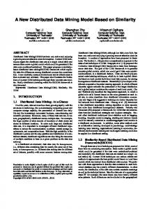
Fig. 1.
A typical distributed data mining environment.
environment. DDM pays careful attention to the distributed resources of data, computing, communication, and human factors in order to use them in an optimal fashion. Figure 1 shows the structure of a typical DDM application that runs over a network of multiple data sources and compute nodes. This paper offers some case studies that involve applications of DDM algorithms for analyzing Earth and Space Science data. Section II presents an overview of some of the emerging DDM applications that are relevant to Earth and Space Science research. Section III describes a specific application of distributed Bayesian networks from NASA and NOAA data sets. Section IV describes another project which is concerned with mining distributed virtual observatories. Finally, Section V concludes this work. II. E MERGING A PPLICATIONS OF DDM This section discusses some general emerging application directions for the field of distributed data mining (DDM). DDM applications come in different flavors. When the data can be freely and efficiently transported from one node to another without significant overhead, DDM algorithms may offer better scalability and response time by (1) properly redistributing the data in different partitions or (2) distributing the computation, or (3) a combination of both. These algorithms often rely on fast communication between participating nodes. When the data sources are distributed and cannot be transmitted freely over the network due to privacy-constraints or bandwidth limitation or scalability problems, DDM algorithms work by avoiding or minimizing communication of the raw data. Both of these scenarios have interesting real-life applications. The
2
Fig. 2. Comparison of the battery power needed to transmit data over CDPD wireless networks with that for performing PCA in a HP Jornada 690 (Hitachi SuperH SH-3 133MHz processor with 32MB RAM running Windows CE). The results clearly show that the power consumed by the onboard computation is a lot less compared to that needed to transmit to a remote desktop machine over CDPD wireless networks.
following discussion offers some of the emerging ones where the DDM technology is finding increasing attention. A. Mobile and Wireless Applications There are many domains where distributed processing of data is a natural and scalable solution. Distributed wireless applications define one such domain. Consider ad hoc wireless sensor networks for applications such as monitoring vegetation or atmospheric characteristics or forest fire-related attributes. Most such applications of sensor networks involve relatively long period of little activities with occasional burst of activities triggered by certain conditions. If continuous monitoring of the incoming data requires non-trivial data analysis then we may need DDM algorithms for minimizing data communication, improving load balance across the network, reducing response time, improving scalability, and minimizing consumption of the battery power. Central collection of data from all the sensor nodes followed by data analysis using standard centralized data mining systems would fail to scale up. This approach is likely to create heavy traffic over the limited bandwidth wireless channels which in turn will offer poor response time and drain a lot of power from the devices. Figure 2 illustrates this point. It shows that the battery power needed to transmit data over a standard CDPD network from one node to another is a lot more than than that needed to perform principal component analysis on the same data set using a HP Jornada 690 (Hitachi SuperH SH-3 133MHz processor with 32MB RAM running Windows CE) system. Further discussion on the power consumption characteristics of popular data mining techniques can be found elsewhere [11]. This result points out that it may be worthwhile to perform some of the data analysis on-board the sensor node, which the DDM algorithms usually adopt, instead of sending all the data to a remote node. Power consumption is not the only issue. DDM over wireless networks also allows the application to run efficiently even in the presence of severe bandwidth constraints. Therefore, it
Fig. 3.
Architecture of the vehicle data mining system.
is not surprising to see a growing number of DDM systems for mobile applications [8], [11]. For example, the distributed vehicle data stream mining system [6] connects to the vehicle data bus in real time and monitors the data using a PDA-based platform and communicates with the remote control station over wireless networks. Figure 3 shows the on-board hardware developed at the DIADIC laboratory of the University of Maryland, Baltimore County and a screen-shot of the desktopbased interface that interacts with the remote on-board devices over wireless networks. This system continuously monitors and mines the on-board data stream generated by the different vehicle systems. The control station allows the user to monitor and mine a large number of vehicles in a fleet. This particular application deals with distributed mobile data sources and static user of the control station. There are also many mobile applications that deal with static data sources and mobile users. The MobiMiner system for mining and monitoring stock market data, reported elsewhere [8], is an example of that. We believe that in the near future we will see more mobile applications of the DDM technology for personalization, process monitoring, intrusion detection in ad hoc wireless networks, and other related domains. B. Large Scale Scientific, Business, and Grid Mining Applications The wireless domain is not the only example. In fact, most of the applications that deal with time-critical or a largequantity of distributed data may benefit by paying careful attention to the distributed resources for computation, storage, and the cost of communication. The world wide web is a very good example. It contains distributed data and computing resources. An increasing number of databases (e.g. weather databases, astrophysical data from virtual observatories, oceanographic data at www.noaa.gov), and data streams (e.g. financial data at www.nasdaq.com, emerging disease information at www.cdc.gov) are coming on-line. It is easy to think of many applications that require regular monitoring of these diverse and distributed sources of data. A distributed approach to analyze this data is likely to be more scalable and practical, particularly when the application involves a large
3
number of data sites. The distributed approach is also finding applications in mining remote sensing and astronomy data. For example, the NASA Earth Observing System (EOS), a data collector for a number of satellites, holds many data sets that are stored, managed, and distributed by the different EOS Data and Information System (EOSDIS) sites that are geographically located all over the USA. A pair of Terra spacecraft and Landsat 7 alone produces about 350 GB of EOSDIS data per day. An on-line mining system for EOS data streams may not scale if we use a centralized data mining architecture. Mining the distributed EOS repositories and associating the information with other existing environmental databases may benefit from DDM [3]. In astronomy, the size of telescope image archives continues to increase very fast as information is collected for new all-sky surveyors such as the GSC-II [9] and the Sloan Digital Sky Survey1. DDM may offer a practical scalable solution for mining these large distributed astronomy data repositories. As mentioned earlier, DDM may also be useful in grid environments [1], [2], [4], [13] with multiple compute nodes connected over high speed networks. Even if the data can be centralized using the relatively fast network, proper balancing of computational load among a cluster of nodes may require a distributed approach. Moreover, a distributed environment requires proper management of other distributed resources like the data, privacy, and collaborative user-interaction. Several new distributed data mining applications belong to this category. The Kensington Enterprise Data Mining System 2 and some of the counter-terrorism applications reported elsewhere [5] belong to this category. There exist several other emerging DDM application areas. Mining distributed multi-party, privacy-Sensitive data is one such example. However, since most of the Earth and Space Science data are not usually privacy-sensitive, we do not discuss this issue in this paper. Interested readers should consult [14] for further details on this topic. The rest of this paper focuses on specific applications of DDM in the Earth and Space Science domain. First, we consider a specific application of Bayesian networks for mining distributed NASA and NOAA data sets in the following section. III. D ISTRIBUTED BAYESIAN N ETWORK L EARNING FROM M ULTI -O RGANIZATIONAL E ARTH S CIENCE DATA In an earlier work [12], we proposed a collective method to address the problem of learning the structure of a Bayesian network from distributed heterogeneous database. In this case, the dataset is distributed among several sites, with different features at each site. The proposed collective structure learning method has four steps: local learning, sample selection, cross learning, and combination. The collective learning method can learn the same structure that obtained by a centralized learning method (which simply aggregates data from all the sites into a single site) with a subset of samples transmitted to a single site. 1 http://www.sdss.org 2 http://www.inforsense.com
We have applied the proposed collective method to a realworld earth science distributed data mining problem. Two distributed datasets, NASA DAO monthly subset and NOAA AVHRR Pathfinder product, are used in this application. The data model are multi-dimension time series (time, longitude, latitude, features). After some preprocessing steps including feature selection, clustering, z-score, and quantization, we coordinate these two distributed datasets and choose a subset of samples that could have a homogeneous pattern. Then we apply the proposed algorithm to this subset of data and learn a �������� . The BN �������� learned from the collective collective BN ��
�� learned from a centralized method is close to the BN method. A. NASA DAO and NOAA AVHRR Pathfinder Datasets In this Earth science distributed data mining application, we use two datasets: NASA DAO subset of monthly means and a NOAA AVHRR Pathfinder product. The data model in these two datasets is multidimensional time series as shown in Figure 4. Each spatial-temporal data point contains a feature vector. longitude • • •
latitude
(f1, f2, …, fn) Jan 1983
Dec 1992
Time
Fig. 4.
Multidimensional time series data model.
NASA Data Assimilation Office (DAO) provides comprehensive and dynamically consistent datasets that represent the best estimates of the state of the atmosphere at that time. The product GEOS-1 uses meteorological observations and an atmospheric model. The dataset used in this application is a subset of the DAO monthly mean dataset. The DAO monthly mean dataset, in turn, is based on the DAO’s full multi-year assimilation. The DAO monthly mean has 180 grid points in the longitude direction from west to east with the first grid point at 180W and with a grid spacing of 2 degrees. There are 91 grid points in the latitude direction from north to south with the first grid point at the 90N and with a grid spacing of 2.0 degrees. The dataset we used from NOAA is a product of NOAA AVHRR Pathfinder. Its format is different from that of DAO dataset: Horizontal Resolution of 1 degree by 1 degree, grid point data (360 x 180 values per level, proceeding west to east and then north to south). B. Preprocessing 1) Feature Selection: There are 26 features in DAO dataset and 9 features in NOAA dataset. However, some features had lot of missing values. One possibility is to use the interpolation technique such as nearest neighbor averaging to handle this problem. However, some features have the missing value at some grid points because these features do not exist
4
TABLE I
Feature Cldfrc in March, 1983 90
NASA DAO FEATURES Description 2-dimensional total cloud fraction Surface evaporation outgoing longwave radiation outgoing shortwave radiation planetary boundary layer depth total precipitation precipitable water net upward longwave radiation at ground net downward shortwave radiation at ground temperature at 2 meters Ground temperature Surface stress velocity vertically averaged uwnd*sphu vertically averaged vwnd*sphu Surface wind speed
Units Unitless mm/day W/m**2 W/m**2 HPa mm/day g/cm**2 W/m**2 W/m**2 K K m/s (m/s)(g/kg) (m/s)(g/kg) m/s
30 Latitude
Feature Cldfrc Evaps Olr Osr Pbl preacc qint radlwg radswg t2m tg ustar vintuq vintvq winds
0
−30
−60
−90
0
30
0.1
60
90
0.2
120
0.3
150
0.4
180 210 Longitude
0.5
240
0.6
270
0.7
300
0.8
330
0.9
360
1
Feature Cldfrc in August, 1983 90
60
30 Latitude
Index 1 2 3 4 5 6 7 8 9 10 11 12 13 14 15
60
0
−30
Index 16 17 18 19 20 21 22
Feature asfts olrcs day olrcs night olrts day olrts night tcf day tcf night
TABLE II
−60
NOAA FEATURES
−90
Description Absorbed Solar Flux total/day Outgoing Long Wave Radiation clear/day Outgoing Long Wave Radiation clear/night Outgoing Long Wave Radiation total/day Outgoing Long Wave Radiation total/night Total Fractional Cloud Coverage day Total Fractional Cloud Coverage night
(undefined) at that grid point. For example, some features from NOAA dataset are only valid over the ocean region. Although other features have values at that grid, these missing value features make the whole record at that grid point useless when we try to build a model to represent the relationship among all variables. So we decided to drop the variable containing a large fraction of missing values. We also dropped some multilayer features and very deterministic features (those that show little variability). After dropping these features, we were left with 15 DAO and 7 NOAA features. These features are listed in Tables I and II. 2) Coordination: The next preprocessing step is to coordinate the distributed NASA DAO/NOAA datasets. It is used to link an observation between the datasets. Since DAO and NOAA datasets have different grid format, we re-grid the NOAA data into DAO format. We selected a common temporal coverage — January 1983 to December 1992 — for the merged dataset (global spatial coverage). Using the mapping key (time, longitude, latitude), we get a distributed database with consistent data format. 3) Clustering: In general, the global dataset does not have a homogeneous pattern. Different spatial-temporal regions may have different patterns. Figure 5 depicts the values of feature Cldfrc(cloud fraction) in March and August, 1983. Clearly, the range of values in tropical and arctic regions are quite different. Also, distributions of the same region for different months are not similar to each other. Using a single BN to model the interaction between the features for the entire earth may not be suitable. Therefore, clustering is first used to segment the spatio-temporal dataset into relatively homogeneous regions. The first step is to aggregate the same month data together. That is, we extract all
0
0
30
Fig. 5.
0.1
60
90
0.2
120
0.3
150
0.4
180 210 Longitude
0.5
240
0.6
0.7
270
300
0.8
330
0.9
360
1
Feature Cldfrc in March (left) and August (right), 1983.
January data for year 1983-1992 and put them into a dataset. This is because of the seasonal nature of the variation in the features (climate behavior is periodic over time). This is a sort of clustering in temporal domain. After that, we need to do spatial clustering. Since the data from first step is for different . time points, we compute the average value and get dataset In , there is no temporal information. Then three clustering algorithms, -mean, fuzzy -mean, and EM, are applied to . The clustering results of DAO and NOAA datasets are shown in Figures 6 and 7. In these figures, same color in same frame means the data points belong to the same cluster. However, similar colors in different frames are irrelevant. The clustering result of DAO and NOAA datasets are consistent. Most data grids in same cluster in DAO have the same labels in NOAA. -mean requires the least computation time and EM can get the best clustering. In our experiment, we used the clustering results of EM. We chose a cluster corresponding to a region of south Pacific ocean (from (170W, 60S) to (90S, 0)) and extracted data in this region to build a BN model. 4) Z-score: Z-score is a standard technique in statistics to transform a random variable into one with zero-mean and unit variance i.e.,
��
�
�
�
�
�
��� � �� �
�
(1)
��
where is the random variable and is the Z-score. 5) Quantization: This step is used to quantize the continuous feature value into discrete values. We use the histogram to quantize the values. If the histogram of is similar to that of a Gaussian curve, we quantize it into 3 levels: 0-low, 1average, 2-high . If resembles a uniform distribution or has two modes, it is quantized into 2 levels: 0-low, 1-high . Note that we do not use more than three quantization levels. The reason for this is that too many quantization levels will lead to a large number of parameters. This makes the BN very
�
���
���
�
�
�
5
complex and hard to do learn. The number of quantization levels for the features used are [3, 3, 3, 2, 3, 2, 2, 3, 2, 3, 3, 2, 2, 3, 2, 2, 2, 2, 2, 2, 3, 3]. Figure 8 shows the histogram of raw, z-score, and quantized value of feature 8 and feature 20.
DAO K−Mean Clustering Result 90
60
Latitude
30
0
−30
Histogram of f8
Histogram of f20
1500
1000
−60
1000 −90
0
30
60
90
120
150
180 210 Longitude
240
270
300
330
500
360
500
DAO Fuzzy C−Mean Clustering Result 90
0 20
60
40 60 80 Histogram of f8 z−score
0 100
100
1500
150 200 250 Histogram of f20 z−score
300
−4 −2 0 2 Histogram of quantized f20
4
1.2
2
1000
Latitude
30
1000 500
0
500 −30
0 −6
−60
−4 −2 0 2 Histogram of quantized f8
0 −6
4
4000 −90
0
30
60
90
120
150
180 210 Longitude
240
270
300
330
360
6000
3000
4000
2000
DAO EM Clustering Result 90
2000
1000 60
0
1
1.5
2
2.5
0
3
1
1.4
1.6
1.8
Latitude
30
Fig. 8.
0
Histogram of feature 8 and feature 20
−30
−60
−90
0
30
Fig. 6.
60
90
120
150
180 210 Longitude
240
270
300
330
360
DAO Clustering results.
NOAA K−Mean Clustering Result
C. Distributed BN Learning
�������
90
60
Latitude
30
0
−30
−60
−90
0
30
60
90
120
150
180 210 Longitude
240
270
300
330
360
NOAA Fuzzy C−Mean Clustering Result 90
60
Latitude
0
−30
−60
0
30
60
90
120
150
180 210 Longitude
240
270
300
330
360
240
270
300
330
360
NOAA EM Clustering Result 90
60
Latitude
30
0
−30
−60
−90
��
��
We compare with to evaluate the performance of collective method. We use structure to describe ����� � and ���
�� difference the similarity between . It is defined as the ��
�� but not in �������� ) and sum of missing links (a link in �� � � � � � � ���
�� ). extra links a link in but not in March dataset was used in the application. It has 9130 samples. The node ordering used was [10 11 8 7 6 3 1 9 14 2 13 5 12 15 16 18 17 20 19 21 22 4]. The centralized ��
�� is very complicated. BN structure is shown in figure 9. It has 64 local links and 9 cross links. The cross links are:
�������� �� � ���� �� ����� �� ��������������������� ����������� �������������������������� . Cross nodes are � ������������� ������ � . In
30
−90
After above preprocessing steps, we have twelve distributed datasets. Each dataset corresponds to a collection of monthly data for year 1983-1992 in a rectangular region from (170W, 60S) to (90W, 0). Each database has 22 features (15 from NASA DAO and 7 from NOAA) and these features are discrete. All samples are complete with no missing value.
0
Fig. 7.
30
60
90
120
150
180 210 Longitude
NOAA Clustering results.
local learning step, there are no extra links. In cross learning step, when we transmit 35% samples, we can get 7 correct cross links and no extra cross links. and are missing. If we transmit 66% samples, we can get all correct cross links and no extra cross links. The collective learning result is in Figure 10. The fact that there are 9 cross links and many local links makes the distributed learning a very hard problem. The performance of collective learning is fairly good, given the complexity. This experiment again demonstrates the effectiveness of collective method.
�� ���
!�"� �
D. Discussion We have presented an approach to learning the structure of BN from distributed heterogeneous data. This is based on a
6
10
2
1
5
13
11
9
6
7
16
14
12
8
3
4
18
15
17
20
19
21
22
��������
Fig. 9.
of March dataset.
NASA DAO/NOAA Structure learning result
��
��
very close to with 40% samples transmitted. This clearly shows the efficiency and accuracy of the collective methods.
6
5
IV. D ISTRIBUTED DATA M INING
OF
A STRONOMY DATA
Structure Error
4
3
2
1
0 0.25
Fig. 10.
0.3
0.35
0.4
0.45
0.5 |Dcoll|/|D|
0.55
0.6
0.65
0.7
0.75
NASA DAO/NOAA structure learning results.
collective learning strategy, where a local model is obtained at each site and the global associations are determined by a selective transmission of data to a central site. In our collective method, local learning can identify the local structure of local variables and local links of cross variables. Cross learning can detect the cross links of cross variables. Combining the results, we can put together the local BNs and the BN learned from cross learning and also remove any “extra” local links. We apply the proposed distributed BN structure learning to NASA DAO monthly subset/NOAA AVHRR Pathfinder Databases. To our knowledge, this is the first research work on distributed BN structure learning from NASA/NOAA Earth science data. Mining distributed Earth science data includes preprocessing techniques which is important for successfully finding the useful patterns. Preprocessing techniques such as feature selection, coordination, clustering, normalization, and quantization ����� � is are introduced. Finally, we learn interesting patterns.
In this section we describe an on-going project in its early stages to explore the use of distributed data mining over a collection of large, geographically distant data repositories containing Astronomy data. While each contains valuable information, the combination contains yet more. Tools for analyzing data in both databases could allow astronomers to make discoveries they could not have made otherwise. The analysis, in principal, could be carried out in a centralized fashion. First download all of the relevant data from each repository to a central site, join to form a single (potentially much larger) dataset, then apply traditional data mining tools. While this solution might be acceptable in some circumstances, it does not offer much room for scalability as in the applications described earlier this paper. The goals of this project are to explore the use of distributed data mining as an alternative to centralizing the data. A primary motivation is the potential for vastly improved scalability. Next we briefly describe the data repositories and the goals of the analysis. Finally we describe key problems that need be overcome to carry-out the analysis without centralizing. A. The Data The Sloan Digital Sky Survey (SDSS)3 and 2 Micron AllSky Survey (2MASS)4 have compiled databases containing well-curated data about millions of astronomical objects. These two databases are located on opposite ends of the U.S. and operate independently. Moreover both are extremely 3 http://www.sdss.org 4 http://irsa.ipac.caltech.edu/applications/Gator/
7
large (470 million+ point sources for 2MASS and 53 million+ objects for SDSS). The data of interest to our project can be conceptually ���� �� thought of as a table in the SDSS with variables �� � � �� �� � � and a table in the 2MASS with variables �� . Each row in both tables represents information about an � � astronomical object. Its �� entries can be thought of as a “location” in the sky, while the others represent wave-band measurements. To combine data across the repositories, rows ���� must be matched according to their �� locations.5 However, the wave-bands by themselves are not of interest, � � � � � � rather their pair-wise differences e.g. , , , , etc.. There are 28 different (unordered) pairs. So, conceptually, each matching pair of rows will generate a 28-dimensional new data point. The 28-dimensional new data points can be thought of as the “signature” of an object.
� � �� � � � � � � � � �� �
� �
�
� �
�
� � �
B. The Data Analysis Goals Objects whose signature stands-out are interesting. Their identification and subsequent more careful examination by astronomers can lead to new scientific discoveries. The primary data analysis goal is to aid the astronomer in identifying objects whose signature stands-out. To do this we intend to explore two types of data mining techniques, clustering and outlier detection. Clustering attempts to find natural groups of points in a body of data. The groups (clusters) contain points which are potentially similar. Those points not falling in clusters can be thought to stand-out. Outlier detection attempts to find directly points which are considerably different than the rest. Of course, a distributed solution would not realize all 28dimensional data points at a central site. Instead such a solution strives to do most of its computation locally and minimize communication. It in known in the distributed data mining field that some problems lend themselves well to distributed solutions. C. Key Problem The main problem we face is that 15 of the 28 features (dimensions) of the signature data are constructed using variables from both datasets. Localizing the computation is a nontrivial task. While the distributed data mining community has considered clustering heterogeneously distributed data,6 the additional twist of constructed difference features makes the problem unique. A simple-minded approach is to first form the local difference sets at each site. The SDSS site will have a difference table with three features and 2MASS with ten features. Next, each local table is clustered. From the local clusterings interesting outliers or isolated clusters can be found. These represent objects which are astrophysically interesting with respect to local data. Finally, centralize the data only for those objects and then compute the ”distributed” SDSS-2MASS differences. 5 If
their locations are “close enough” the rows are deemed a match. a table that has been split vertically with columns spread over remote sites 6 conceptually
The advantages of the above approach are simplicity and low communication cost – messages are only required for the data representing astrophysically interesting objects which is likely to be small. The primary disadvantage is that the results are incomplete. Since the clustering and outlier finding is applied to local data, interesting clusters/objects may be missed. For example, if an interesting cluster does not manifest itself on either local difference table, then it will be missed. We are also actively pursuing a distributed approach that can account for the distributed differences (15 features). However, the problem seems to be unique in the DDM literature, so we may need to develop a completely new method. While difficult, this is an exciting prospect as it opens new ground to explore in DDM. V. C ONCLUSION In this paper we discussed the emerging field of distributed data mining (DDM) and some applications in earth and space science. A common situation involves multiple, large, geographically distributed data sites. Analysis over all data sites could provide valuable information that could not be learned from any site individually. However, centralizing all of the data to one site is not a feasible option (due to bandwidth constraints, privacy, etc.). A DDM approach attempts maximize the amount of analysis done locally at each site and minimize communication between. The main part of this paper discusses an application of DDM on two distributed earth science datasets: NASA DAO monthly subset and NOAA AVHRR Pathfinder product. The technique constructs a Bayesian network without having to centralize the data, but merely sending a sample. Empirical results show that good accuracy can be obtained with modest sample sizes. The last section (before conclusion) discusses the preliminary stages of an application of DDM on space science datasets: Sloan Digital Sky Survey and 2 Micron All-Sky Survey. The end goal of the application is a method for identifying astronomical objects which “stand-out” from the rest. These objects, when examined more closely by astronomers, can lead to interesting scientific discoveries. In conclusion, we believe that DDM has valuable potential in Earth and space science. This is particularly true as the data sets accumulated by scientists continue to grow in size. We encourage scientists to explore applications of DDM in their domains. VI. ACKNOWLEDGMENTS We would like to thank NASA for funding through grant (NRA) NAS2-37143. We would also like to thank Kirk Borne for several useful discussions concerning distributed data mining of SDSS and 2MASS astronomy data. R EFERENCES [1] G. Agrawal. High-level Interfaces for Data Mining: From Offline Algorithms on Clusters to Streams on Grids. In Workshop on Data Mining and Exploration Middleware for Distributed and Grid Computing, Minneapolis, MN, September 2003. [2] M. Cannataro, D. Talia, and P. Trunfio. KNOWLEDGE GRID: High Performance Knowledge Discovery on the Grid. GRID 2001, pages 38–50, 2001.
8
[3] R. Chen, B. H. Park, K. Sivakumar, H. Kargupta, J. Ma, and M. Da. Distributed data mining for nasa/noaa databases, December 2002. AGU Fall 2002 meeting, San Francisco. [4] A. Chervenak, I. Foster, C. Kesselman, C. Salisbury, and S. Tuecke. The Data Grid: Towards an Architecture For the Distributed Management and Analysis of Large Scientific Datasets, 1999. [5] R. Grossman. Finding bad guys in distributed streaming data sets. Panel Presentation on Resource and Location Aware Data Mining, Second SI AM International Workshop on High Performance Data Mining. [6] H. Kargupta, R. Bhargava, K. Liu, M. Powers, P. Blair, and M. Klein. VEDAS: A Mobile Distributed Data Stream Mining System for Real-Time Vehicle Monitoring. In Proceedings of the 2004 SIAM International Conference on Data Mining, 2004. [7] H. Kargupta, B. Park, D. Hershberger, and E. Johnson. Collective Data Mining: A New Perspective Towards Distributed Data Mining. In Hillol Kargupta and Philip Chan, editors, Advances in Distributed and Parallel Knowledge Discovery, pages 133–184. MIT/AAAI Press, 2000. [8] H. Kargupta, K. Sivakumar, and S. Ghosh. Dependency Detection in MobiMine and Random Matrices. In Proceedings of the 6th European Conference on Principles and Practice of Knowledge Discovery in Databases, pages 250–262, Helsinki, Finland, 2002. Springer Verlag. [9] B. McLean, C. Hawkins, A. Spagna, M. Lattanzi, B. Lasker, H. Jenkner, and R. White. New horizons from multi-wavelength sky surveys. IAU Symposium. 179, 1998. [10] B. Park and H. Kargupta. Distributed Data Mining: Algorithms, Systems, and Applications. In Nong Ye, editor, Data Mining Handbook, pages 341–358. IEA, 2002. [11] R. Bhargava and H. Kargupta and M. Powers. Energy Consumption in Data Analysis for On-board and Distributed Applications. In Proceedings of the 2003 International Conference on Machine Learning workshop on Machine Learning Technologies for Autonomous Space Applications, 2003. [12] R. Chen and K. Sivakumar and H. Kargupta. Collective mining of Bayesian networks from distributed heterogeneous data. Knowledge and Information Systems, 6:164–187, 2004. ´ cin, M. Ghanem, Y. Guo, M. K¨ohler, A. Rowe, J. Syed, and [13] V. Curˇ P. Wendel. Discovery Net: Towards a Grid of Knowledge Discovery. In Proceedings of the Eighth ACM SIGKDD International Conference on Knowledge Discovery and Data Mining, pages 658–663, Edmonton, Canada, 2002. ACM Press. [14] V. Verykois, E. Bertino, I. Fovino, L. Provenza, Y. Saygin, and Y. Theodoridis. State-of-the-art in Privacy Preserving Data Mining. SIGMOD Record, 33(1):50–57, 2004.