of m equations and p unknowns, so it is possible to recover the checkpoint data of the p failed nodes. Plank proposes a method for generating good Cauchy ...
Distributed Diskless Checkpoint for Large Scale Systems Leonardo BAUTISTA GOMEZ1,3 , Naoya MARUYAMA1 , Franck CAPPELLO3,4 , Satoshi MATSUOKA1,2 1 Tokyo Institute of Technology - 2 National Institute of Informatics 3 INRIA – 4 University of Illinois at Urbana Champaign Abstract—In high performance computing (HPC), the applications are periodically checkpointed to stable storage to increase the success rate of long executions. Nowadays, the overhead imposed by disk-based checkpoint is about 20% of execution time and in the next years it will be more than 50% if the checkpoint frequency increases as the fault frequency increases. Diskless checkpoint has been introduced as a solution to avoid the IO bottleneck of disk-based checkpoint. However, the encoding time, the dedicated resources (the spares) and the memory overhead imposed by diskless checkpoint are significant obstacles against its adoption. In this work, we address these three limitations: 1) we propose a fault tolerant model able to tolerate up to 50% of process failures with a low checkpointing overhead 2) our fault tolerance model works without spare node, while still guarantying high reliability, 3) we use solid state drives to significantly increase the checkpoint performance and avoid the memory overhead of classic diskless checkpoint.
I. I NTRODUCTION Parallel scientific applications can spend days or even weeks in execution. Long executions must be checkpointed periodically to increase their success rate. In the classic diskbased approach, all processes will be coordinated to capture a consistent state of the parallel execution and then the state of all processes will be stored on stable storage. When the execution is restarted after a failure, the context of the parallel execution is restored from the disk. When a system with tens of thousands of processes tries to write the checkpoint data to stable storage the IO bandwidth will be saturated creating an IO bottleneck. The overhead caused by the IO bottleneck of this technique can be as large as 20% of the execution time [3, 17], and it will increase dramatically in the next years. Diskless checkpoint [1] has been proposed as a solution to avoid the IO bottleneck of disk-based checkpoint. Diskless checkpoint uses several encoding techniques and extra resources to avoid writing in disks. The encoding techniques, such as XOR or Reed Solomon, generate some encoded data that will be stored in the main memory of dedicated nodes and used to recover the lost data in case of failure. However, diskless checkpointing suffers from several issues limiting its scalability: • Most of the encoding techniques can tolerate only 1 or 2 simultaneous process failures (See Section III). • Encoding algorithms capable to tolerate more than 2 simultaneous process failures are highly time and memory consuming[11, 12, 13].
• •
•
Most of the diskless checkpoint models require spare nodes[1] and dedicates processors. Diskless checkpoint is unable to restart the execution after a whole system failure if process checkpoints are stored in volatile memory. The approach stores encoded data in main memory which decreases the applications’ performance by reducing the available capacity.
A. Contributions Our objective is to create a highly scalable, fault tolerance model that allows applications to tolerate several simultaneous failures while avoiding the 3 main issues of diskless checkpointing presented above. •
•
•
•
•
We propose a fault tolerant model with a low checkpoint overhead, capable to tolerate simultaneous failures up to 50% of all processes engaged in the parallel execution. Also, our model presents a partitioning and mapping technique aimed to avoid spares. With this model we introduce a new concept: the failure distribution strategy which increases the capability to tolerate high fault rates by virtually dispersing the failures in different groups and sectors (See Section IV). We present an encoding algorithm of the weighted checksum encoding, specially designed to optimize the encoding process in our fault tolerance model. Our evaluation shows how our model scales to almost 200 nodes and 900 processes. We use SSDs to solve the memory overhead induced by the classic diskless checkpoint and demonstrate how they increase the checkpointing performance. We present several recovery strategies and we explain how our model can tolerate a whole system failure and even more failure scenarios than the disk-based checkpoint technique.
The rest of this paper is organized as follows. Section II presents the failure background in HPC. In Section III, we discuss some related works and their limitations. Section IV presents our fault tolerance model and introduces the SSDs. In Section V we present the implementation of our encoding algorithm. In section VI we evaluate the scalability of the presented model and the proposed encoding algorithm. Section VII concludes the paper and discusses future work.
II. BACKGROUND Nowadays, the scientists use supercomputers for a large variety of scientific purposes such as global climate modeling, computational fluid dynamics and biomedical imaging. Supercomputers can execute scientific applications with thousands of processes and these applications can spend days or even weeks. However, the success of long executions depends on the reliability of the system. In systems with more than ten thousands processors, the mean time to failure (MTTF) drops to less than ten hours and even for a system based on ultrareliable components, the MTTF is less than twenty hours [4]. The number of processors in supercomputers is increasing and will continue to increase in the next years. In 2012, systems with hundreds of thousands of processors will have a MTTF of only a few hours [3, 17]. Most of the scientific applications deployed on supercomputers can fail if only one of its processes fails. In HPC, parallel applications deal with failures by periodic checkpointing. There are several checkpointing techniques; in the most popular approach, all processes coordinate to store the application context to stable storage. When a failure occurs, the execution is restarted from the last checkpoint. However, in large scale systems, comprising tens of thousands of processors, the size of the checkpoint data may exceed tens of tera bytes and can easily saturate the network and storage farm, creating an IO bottleneck. This leads to poor checkpointing performance and increases the checkpointing interval. In this context, it is important to improve the checkpointing performance to decrease the overhead and keep low the influence of the checkpoint time in the calculation of the checkpoint interval for a given MTBF [18]. The rest of this section discusses the failures in HPC and presents the classic disk-based checkpointing approach. A. Analyzing failures in HPC A very large study of failures [3, 17] shows that in more than 60% of failures the root cause is hardware when only in less than 25% the root cause is software. This study has been done using data collected over 9 years at Los Alamos National Laboratory (LANL). It covers 23000 failures collected from 22 HPC systems, counting in total more than 24000 processors. This work shows that the variability in failure rate is high when the systems vary widely in size. Also, this study reports that some systems experienced a large amount of simultaneous failures. This high rate of simultaneous failures between two or more nodes indicates a tight correlation between nodes. Correlated failures are an important factor [24] to analyze in order to build a realistic checkpointing model able to tolerate a high number of simultaneous process failures. B. Disk-based approach limitations Fig. 1 illustrates a balanced architecture for Petascale computers composed of computing nodes, IO nodes and the parallel file system. The total memory of the computing nodes is around 100 and 200 TB. The parallel file system has around 2 PB and the IO bandwidth is between 40 to 200 GB/s.
Fig. 1.
Balanced architecture for PetaScale computers
In this context, we can easily understand why storing about 100 to 200 TB of checkpoint data can take more than 1000 seconds. In order to increase the success rate of long applications, current systems have a checkpoint interval of one hour, generating a checkpointing overhead of more than 20% for current scientific applications [15]. Some dedicated file systems such as PLFS [26] have increased dramatically the checkpoint performance for a large range of applications. However, the presented classic approach has serious limitations. The number of nodes and the memory of new supercomputers are increasing, then the size of checkpoint data is increasing too and the MTBF is decreasing. The new systems will have to checkpoint more often and more data [24]. With the classic disk-based approach, these constraints impose a high checkpointing overhead increasing the time to solution of scientific applications. III. R ELATED WORK Several techniques to improve the checkpointing performance have been proposed, such as incremental checkpoint with the Libckpt library [9], and speculative checkpoint [10], which is an attemp to exploit temporal reduction in system level checkpointing. In other words, between the intervals of coordinated checkpointing, the user or the system will speculatively predict whether it will be the last write prior to the next checkpoint and thus can be speculatively checkpointed early. However, the effectiveness of incremental checkpoint will depend on the memory usage of the application. In the same way the effectiveness of speculative checkpointing is greatly affected by the last-write heuristics. Nowadays, the BLCR [5, 6, 7, 8] library implements kernel level checkpoint and is used in some production clusters. Diskless checkpoint [1, 4, 14] is a technique that uses main memory and available processors to encode and store the encoded checkpoint data. The aim of diskless checkpoint is to avoid the IO bottleneck of disk-based checkpoint. To accomplish this goal, it proposes several techniques. First, the checkpoint data is not stored on remote distributed storage but
in the main memory or local disk. Checkpointing on the local memory raises the issue of checkpoint availability in case of node failure. In order to guarantee a high level of reliability, several strategies have been proposed such as storing the checkpoint on neighbor nodes [14] and use redundancy codes and spare nodes. Finally, the system can be partitioned in groups in order to deal with scalability and to increase the failure tolerance rate. This section briefly reviews previous diskless checkpoint approaches and encoding techniques.
a large study of these libraries is done and a performance comparison between encoding techniques is presented. The results show that special-purpose RAID-6 codes outperform general-purpose codes. However, these RAID-6 codes only tolerate two erasures. The authors stated that the place where future research will have the highest impact is for larger values of m (erasures tolerated). Unfortunately, all these libraries are designed for storage purpose and not for fault tolerance in HPC.
A. Encoding techniques
C. Localized weighted checksum
The first and simplest encoding technique is parity (RAID5). In this method, the Jth bit of the encoded checkpoint is calculated as the exclusive-OR (XOR) operation between the Jth bit of the checkpoints of all computing nodes. After a failure the checkpoint of the failed node is calculated from the encoded checkpoint and the checkpoints of non-failed processors. This technique tolerates one single failure. In case of two or more failures, the encoded checkpoint and the checkpoint of non-failed nodes will form a system of one equation and two or more unknowns, so it is impossible to recover the data of failed nodes. The one-dimensional parity strategy bypasses the low failure tolerance of the RAID technique [14, 26]. The encoding system is the same (XOR), but the computing nodes are partitioned in groups. Each group has an encoding node in order to tolerate one single failure per group, if there are m groups in the system, then the system can tolerate up to m failures (one per group). However, if there is more than one failure in one group, it is impossible to restart the execution. To solve the problem of more than one single failure tolerance per group, the two-dimensional parity proposes to organize the computing nodes in a matrix and to designate an encoding node per row and per column, and then the system can tolerate several failures per column since the row encoding node can be used to recover the data. In the same way, it is possible to tolerate several failures per row and use the encoding nodes of columns to restart the execution. However, if the number of simultaneous failures exceeds 2, some data will not be recoverable and the application execution will fail. The Reed Solomon (RS) [12, 13, 20] coding has the largest coverage of failures per encoded checkpoint but its encoding method is the most time consuming because of the large amount of encoded checkpoints generated. If there are m encoding nodes then the system tolerate m failures. This technique is similar to the checksum scheme presented above but uses a distribution matrix creating a system of m equations. After p failures, if p ≦ m the system is composed of m equations and p unknowns, so it is possible to recover the checkpoint data of the p failed nodes. Plank proposes a method for generating good Cauchy matrix with better encoding performance [11].
Chen and Dongarra proposed a scalable encoding approach [2] for tolerating more than 3 process failures in large scale systems. Their proposal is to implement a chain-pipeline to encode the checkpoints. The classic algorithm used to encode the checkpoints with the bit parity technique is a binary tree. The authors claim that their technique is scalable in the sense that the overhead to survive k failures in p processes does not increase as the number of processes p increases. To prove it, they demonstrate how the complexity of their algorithm is independent of the number of processes p. The pipeline approach seems to be very interesting to bit parity encoding. However, assuming checkpoint files of size s bytes, the localized √ weighted checksum model proposed in this paper can tolerate k process failures in a group of k processes and requires 2 ∗ s bytes per process. In addition, no failure distribution strategy is proposed to increase the capability to tolerate high fault rates of the model and the evaluation presented is done with checkpoint files of 25MB, wich is unrealistically small for a HPC application.
B. Erasure coding libraries Several erasure coding libraries have been implemented and propose a wide variety of encoding techniques. In [13],
D. The SCR library The Scalable Checkpoint/Restart (SCR) library[16] uses the XOR encoding technique and stores the encoded checkpoints in the computing nodes avoiding spare nodes. The checkpoints are stored on RAM discs. However, this strategy uses the main memory to store the checkpoint and can tolerate only one single process failure in a XOR group of size k, while it requires s + 2∗s k bytes of storage space per process. IV. T HE FAULT TOLERANCE MODEL The approaches presented in the previous section use different strategies to deal with failures. The localized weighted checksum (LWC) and the SCR library propose strategies to avoid spare nodes. We present in this section a distributed diskless checkpoint (DDC) approach avoiding spare nodes and improving previous encoding approaches by tolerating 100% of process failures per group in some cases, while requiring only 2 ∗ s bytes of storage space per process A. Tolerating 100% of faults in groups In HPC, the RS encoding or weighted checksum, is highly time consuming because the complexity of the encoding process is related to the group size (See Section V). Thus, the whole system is usually partitioned in groups. Each group will have k processes (k checkpoint files) and will generate
m encoded checkpoints. Usually, the encoded checkpoints are stored on spare nodes, so the group will have k computing processors and m encoding processors. As an example, let us consider a system with k processors. If we want to tolerate k 10% of process failures, we will need m = 10 spare nodes to encode and store the encoded checkpoints. In order to avoid the need for dedicated processors, we could propose to use the computing processors as the encoding processors and then store the encoded checkpoints in the same physical memory where the others “classic” checkpoints are stored. Then, to tolerate m < k process failures each group has m processors used for computing and encoding, and k − m processors used for only computing. In this case, if one of the processors that are used for both (computing and encoding) fails, then we will lose a classic checkpoint and an encoded checkpoint leading to two erasures. In other words, one single processor failure can imply two unknowns in the equation system. In the worst case of m failures, all the computing/encoding processors will fail, then we will have a system of m equations and 2 ∗ m unknowns and it will be impossible to recover the lost data, as result, each group can tolerate just m2 processor failures in the worst case. In conclusion, storing the encoded checkpoints in the computing processors decreases the capability to tolerate high fault rates. On the other hand, if the groups use spares and tolerating a high fault rate is needed, the system will need a large number of spare nodes. For example, if we want to reach a failure tolerance of 100% (m = k), each group have to generate m encoded checkpoints and store them in m spares. These dedicated processors will be used just for encoding purposes and will not participate in the application. As presented above, the first proposition decreases the capability to tolerate high fault rates and the second proposition increases the number of dedicated resources. However, if we combine both propositions, in other words, if we use the computing processors as encoding processors and at the same time we generate one encoded checkpoint for each classic checkpoint file (m = k), no dedicated resource will be needed and the failure tolerance will be m2 , but since m = k the group will be capable to tolerate 50% process failures. Using the presented strategy, we avoid the dedicated processors and we guarantee the capability to tolerate high fault rates. As we explained, one processor 1 failure will imply two erasures in the same group, because for each process we will have a classic checkpoint and an encoded checkpoint, both belonging to the same group. By dispersing the encoded checkpoints in another group we avoid the double-erasure implied by one processor failure. Then, the groups can create a virtual ring and store the encoded checkpoints of the group Gi in the processors of the group Gi+1 . In this way, after a processor failure belonging to the group Gi we will lose one local checkpoint (group Gi ) and one encoded checkpoint of the group Gi−1 . If all the processors of group Gi fail 1 In
this section we use the term processor as a unit of computation with its corresponding memory and belonging one application process.
simultaneously, and we assume there are no failures in group Gi+1 , it is possible to recover all the checkpoint files of the group Gi since the m encoded checkpoints of the group Gi are stored in the group Gi+1 . Also, we will lose all the encoded checkpoints of the group Gi−1 but if we assume there are no failures in the group Gi−1 , then the processes of group Gi−1 just have to regenerate their encoded checkpoints. In the worst case, independently of the system size or the number of groups, the system will be capable to tolerate only m processor failures. However, in HPC most of the failures affect only one or some few nodes [3, 17, 24] and using the strategy presented in this section the failures will be distributed among the groups. Since the groups disperse the encoded checkpoints in the neighbor groups, the fault tolerance of a group will depend on the fault rate of its neighbors. Two consecutive groups will be capable to tolerate up to 50% local processor failures and if the failures are perfectly distributed among the groups then the whole system too will be capable to tolerate up to 50% processor failures. Furthermore, when the neighbors of a given group have no failures, the group can tolerate up to 100% local processor failures. In this way, we can build a spare-free fault tolerance model capable to tolerate 100% of processor failures per group and it requires no more than 2 ∗ s bytes per process. B. Partitioning the system in groups In order to increase the capability of the whole system to tolerate high fault rates, the process failures should be distributed among the groups. In modern multiprocessor, multicore nodes, the failure of a single node implies the failure of several (4, 8 or more) processes, thus if all the processes of a node belong to the same group, a node failure will imply several erasures within that group. On the other hand, if we distribute all the processes of one node among different groups, then one node failure will imply one single process failure in several groups, instead of several process failures within the same group. In the former distribution approach, the reconstruction of failed processes is distributed among several groups while in the later approach the reconstruction migh be impossible because there is not enough remaining information in a single group to reconstruct the failed processes.
Fig. 2.
Groups building strategy
Fig. 2 shows an example with 8 nodes of 4 processors (4 processes per node). Using this strategy, we will create 4 groups (4 colors) of 8 processors each. When a node fails,
each group will have one processor failure, which is the best possible distribution of the failures among the groups. This system can tolerate up to 4 node failures (16 processor failures) and it will be able to recover the lost checkpoints in all the groups. The encoding process will be significantly faster for 4 groups of 8 processors than for 1 group of 32 processors because the groups can encode in parallel (See Section V). When the groups are built using the presented strategy, the failures will be distributed among the groups then we can use small groups to encode; but as we mentioned in Section II, the failures can affect several nodes and if the groups are smaller than the number of failed nodes, the system will be unable to recover the data. It is important to find a group size that guaranties a good tradeoff between encoding speed and capability to tolerate high fault rates. We studied the failures records of Tsubame [21] for the last two years and we found that 98% of failures affect less than 4 nodes simultaneously. This does not mean that the group size should be 4 for every supercomputer. Other supercomputers, may have a different number of failures and will need different group sizes. However, even if the number of failures increases linearly with the system size, the number of nodes affected per failure should not increase that fast. If the average number of nodes affected per failure remains constant, then the group’s size can remain constant and then the encoding time and the checkpointing performance will remain constant. Using this model, every supercomputer administrator can choose the size of the groups to tolerate a percentage X% of failures and perform a fast encoding, after careful study of his system.
Fig. 3.
Partitioning the system in sectors and groups
According to the strategies mentioned above, the partitioning technique will be as follows: let us imagine a system with P nodes. In every node, H processes are running and the application has a total of N = P * H processes. In this system, suppose that a high percentage of failures (X%) affect less than M nodes. Then, we will create groups of M processes. All the processes in a group must be from different nodes. We will divide the whole system in sectors. A sector is a group of M nodes. Please note that a sector is not a group of processes. A sector can be viewed in hardware level as a group of nodes and in a virtual level as a group of groups. For simplicity we assume that P is divisible by M. In a sector, we will have H groups of size M and a sector will have M * H processes. Fig. 3 shows an example of this partitioning technique for a system with 8 nodes (P = 8), 2 processes per node (H = 2) and the system administrator knows that 95% of failures affect no more than 4 nodes (M = 4). Following the partitioning steps presented above, the administrator will create groups of size 4
(M) and sectors of 4 (M) nodes, the sector A with the nodes A1 to A4 and the sector B with the nodes B1 to B4. There will be 2 (H) groups per sector, the groups G1 and G2 belonging to sector A and the groups G3 and G4 from sector B. C. Positioning the groups on the ring In Section IV.A we explained how to build a system where each group can tolerate up to 100% of failures assuming that the neighbor groups does not have any failure. However, if all the groups of a same sector are in a contiguous part of the ring, then when a group has a process failure because of a node failure, its neighbors will have a process failure too. For example, using the system of Fig. 3, let us consider the following ring (G1 – G2 – G3 – G4). When one node of sector A will fail, for example A2, then G1 will have a process failure and its successor, G2 will have a process failure too. G1 can not tolerate 100% of process failures because G2 will have some process failures too. Since the encoded checkpoints of the group G1 are stored in the group G2, the processor failure in the group G2 implies to lose an encoded checkpoint of the group G1, resulting to a lower fault tolerance. On the other hand, if we intercalate groups of different sectors among the ring, the groups can easily reach the maximum fault tolerance rate of 100%. Let’s study this second ring: (G1 – G3 – G2 – G4), using the same system of Fig. 3. In this second case, when one node fails, for example the node A2, then the same groups G1 and G2 will have a process failure. But instead of having a process failure in two consecutive groups, the neighbors of groups G1 and G2 (G3 and G4) will not have any process failure, then the group G1 and G2 will have the capability to tolerate higher fault rates. Using this positioning strategy, we can distribute the correction of failure effects in the ring. Now assume that the nodes A1, A2 and A3 belong to the same Triblade module and the whole Triblade module fails. This means 3 node failures or 6 process failures. Given the groups G1 to G4, the SCR library could not tolerate this scenario of failures, neither the localized weighted checksum model; on the contrary, using the strategies presented above, our model can tolerate this Triblade module failure and can even tolerate a failure of four nodes whichever they are. D. Avoiding the memory overhead The fault tolerance model presented in this section increases the capability to tolerate high fault rates and eliminates the need for dedicated resources. However, this technique will generate one checkpoint file and one encoded checkpoint for each process. If all these checkpoints are stored in the main memory the application may start to swap and the performance will decrease dramatically. In order to avoid the memory overhead imposed by our model, we propose to use SSD devices. The SSDs are data storage devices that use solid-state memory to store data persistently. The SSDs have the advantage of being electronic devices instead of electromechanical devices (no moving parts) such as classic
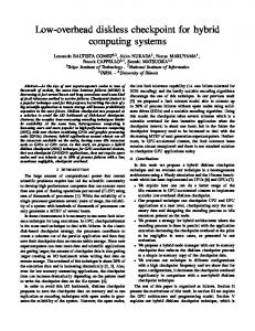
Hard Disks Drives (HDDs). For this reason, SSDs are less fragile, silent and faster than HDDs. We propose to use this technology to store the checkpoint data. Using SSDs to store the checkpoints and encoded checkpoints we avoid the memory overhead produced when storing the checkpoint data in the main memory. In addition, the SSDs can be several times faster than the classic HDDs which will increase the checkpoint performance. In order to determine the speedup of using SSD we made some experiments with classic HDDs, a Super-talent SSDs and an ioDrive. For our experiments we used a Western Digital HDD with a spindle speed of 7,200RPM, an average rotational latency of 4.20ms and a cache size of 16MB plugged on the Serial ATA interface. The Super-talent SSD also uses the Serial ATA interface, has an internal cache of 64MB and a latency of 0.1ms. The ioDrive is a new SSD with an average access latency of 30µs connected by a four lanes PCI express 2.0.
will depend on the group size and checkpoint size. The coordinated checkpointing time into local disk will depend on the coordination time and the device speed. Table 1 shows the local writing performance using HDD, SSD and ioDrive for different checkpoint data sizes. Furthermore, on Table 1 we can see that in the 32GB case the local writting process takes almost 10 minutes using HDD and less than one minute using ioDrive; assuming a checkpoint interval of one hour, the local writting process will lead to an overhead of 16.1% using HDD and only 1.2% using ioDrive. On the other hand, using SSDs on the nodes could decrease the reliability of the system significantly. We do not know about any failures study done on a large scale system with SSDs on the computing nodes, so it is difficult to predict exactly the impact of introducing this new technology. However, our model is specially designed to tolerate a large amount of simultaneous failures, including SSD failures. Ckpt. data size 8GB per node 16GB per node 32GB per node
HDD 55MB/s 145 sec. 290 sec. 581 sec.
SSD 215MB/s 37 sec. 74 sec. 148 sec.
ioDrive 685MB/s 11 sec. 23 sec. 46 sec.
TABLE I C HECKPOINTING IN LOCAL DISK
E. The recovery system
Fig. 4.
Write speed of HDD, SSD and ioDrive
The next comparison has been done using the iozone software [23] which is a standard for IO benchmarks. The comparison presents the performance of the standard HDD, the Super-talent SSD and the ioDrive. The benchmarks were realized on the same machines with the same software in the same conditions. The comparison has been done for four different kinds of access: Write, Re-write, Read and Re-read but for brevity we only show the results of the Write test, since the other tests show similar results. Iozone tests the speed of a device using a large range of file sizes and a large range of record sizes for each file size. The file sizes vary between 16MB and 16GB and the record sizes vary between 64KB and 16MB. The write test measures the performance of writing a new file. Fig. 4 shows clearly the different performances between the three different devices. We can see that both SSDs, with write speeds of 215MB/s and 685MB/s for the ioDrive, outperform the HDD with a write speed of only 55MB/s. There are two main, time consuming, steps in our checkpoint model: to checkpoint the context of the distributed application into local disks and to encode the checkpoints to guarantee a high level of reliability. The encoding time
The checkpoint model presented in this section is designed to tolerate a high rate of failures (See Section IV.B) but not 100% of failures. Indeed, when the number of simultaneous failed nodes is larger than the group size, the encoded checkpoints generated may not be enough to recover the lost checkpoints and then the system will be unable to restart the execution. One classic example of this is the well known power outage failure. When all the nodes fail simultaneously, the unique solution to restart the execution is to repair the nodes and restart from the last checkpoint if this checkpoint was stored on stable storage. There is no encoding/decoding algorithm associated with checkpointing on volatile memory capable to tolerate a failure of the whole system. When a failure affect less than 50% of nodes and the failures are well distributed, the system may be able to recover the lost checkpoints using the decoding algorithm. We call this case, the fast recovery. The decoding algorithm, that is similar to the encoding algorithm, is a matrix-vector multiplication regenerating the lost checkpoints. First, the system has to detect the lost checkpoints and inverse the distribution matrix used on the encoding process. Then, the multiplication of the inversed matrix and the checkpoint of non-failed nodes will regenerate the lost checkpoints. Every group will regenerate only the lost checkpoint which will be less or equal to the encoded checkpoint generated per group. In other words, the decoding process will be in the worst case, as long as the encoding process. In this failure scenario, the encoded checkpoints generated by the encoding process guarantee the regeneration of the lost data and once the decoding process is finished, the
execution can restart immediately if the system has the needed number of nodes available. We want to highlight that in this scenario it is not necessary to repair the failed nodes to restart the execution. As explained in Section II, the average number of nodes affected by a failure depends of several factors like the system size, the age of the system, etc. However, most of the failures affect just one or some few nodes [3, 17, 24]. For this reason, it is likely that the fast recovery will be the most commonly used technique to restart the execution. When the number of nodes affected per failure is larger than 50% of nodes or the failures are not well distributed, the system will be unable to recover the lost checkpoint data using the decoding process. The unique solution is to recover the lost checkpoint files from the stable storage. Since we propose SSDs to store the checkpoint files and encoded checkpoint files, we should be able to recover the data after repairing the nodes unless the SSDs themselves had failures. We call this the slow recovery because it is necessary to repair the failed nodes to restart the execution. Obviously, the decoding process is not needed in this case. We want to highlight that, by using SSDs for this checkpoint model, the system can tolerate a failure of the whole system like a power outage, which was not possible in the classic diskless checkpoint. In the precedent scenario it is necessary to use the slow recovery, but in some cases one or several SSDs can be part of the failure. In such cases, it is still possible to restart the execution. Using the decoding process after repairing the nodes. Indeed, since the encoded checkpoints are also stored on stable storage, the checkpoint files lost after the SSD failures can be regenerated using the decoding process. This recovery strategy allows us to restart the execution even in some extreme failure cases that the classic disk-based checkpoint is not able to tolerate. Since most of the storage systems use RAID5 or RAID6 encoding to tolerate one or two disk failures, when more than two disks fail simultaneously, some data will be completely lost. For example, when a failure affects several nodes and several disks simultaneously, the disk-based checkpoint technique will be unable to tolerate such a failure. Instead, using our approach, the system can tolerate up to 50% of disk failures if the failures are well distributed. Since a strong encoding process is used to generate a large number of encoded checkpoints, we just need to launch the decoding process after repairing the nodes to regenerate the original checkpoint files lost. V. T HE ENCODING PROCESS RS encoding algorithm [12, 19, 20] uses a matrix-vector multiplication for its encoding process and can be viewed as a weighted checksum encoding algorithm. The weighted checksum algorithm is an encoding technique which uses a distribution matrix for encoding a data vector. In diskless checkpoint, this data vector is formed by the checkpoint files to encode. A checkpoint file can be viewed as an array of type double or as a bit stream. If it is viewed as an array of type double, then every process Pi will have an array of type double Chi : as checkpoint file. We call Chi j the
jth element of checkpoint file Chi: . If the application has k processes, then the data vector’s size will be k; so the first data vector V1 is composed of the first element of every checkpoint file: < Ch11 ,Ch21 , . . . ,Chk1 >; the second data vector will be formed by the 2nd number of every checkpoint file and so on. In order to generate m encoded checkpoints the distribution matrix will have k + m rows and k columns. As we can see in Fig. 5, this matrix is divided into two parts; the first part (k ∗ k) is an identity matrix and the second part (m ∗ k) is a matrix M (in red) with some mathematical properties. To be able to recover up to m failures, this matrix has to satisfy the condition that any sub-square matrix (including minor) is non-singular. Any Vandermonde matrix and any Cauchy matrix satisfy this condition.
Fig. 5.
RS encoding system
The product between the identity matrix and the data vector does not need to be done because we will get the same data vector. The product between the row i of the matrix M and the data vector V j will produce the encoded value Ci j . So, for a data vector V j we will have the next equation’s system M11Ch1 j + M12Ch2 j + · · · + M1kChk j = C1 j .. .. . . M Ck + M Ch + · · · + M Ch = C m1
1j
m2
2j
mk
kj
mj
where Mi j is the value of row i and column j of M, Chi j is the jth value of the checkpoint Chi: and Ci j is the ith value of the encoded vector C j . Each vector V j will be multiplied by the distribution matrix to get the correspondent encoded vector < C1 j ,C2 j , ...,Cm j >. This computation will be done for every data vector until the last one to get the same number of encoded vectors. We designed an algorithm optimized for the topology of our model, we called it the star algorithm.
A. Implementing the star algorithm Analyzing this equation’s system we can see that all the values of the checkpoint file Chi: will always be multiplied by the values of the same column Mxi of the matrix M. Using this observation, we will distribute each column i of the matrix M to the processor of process Pi , in this way each processor will have its checkpoint file Chi: (or double array) and a column of the matrix M.
data to its successor pi+1 , in the second step to pi+2 and so on, as presented on Fig. 6. To limit the memory usage we break the checkpoint files in t blocks of size z. Fig. 7 illustrates the message transfers for a block encoding within a 5-process group. Arrows of the same color represent parallel communications. This communication pattern similar to a star will be present on every group and the groups will be organized in a virtual ring, creating in this way, a ring of stars.
for i in 1 to t r e a d n e x t b l o c k from Ch : for j in 1 to m for h in 1 to z r e s [ h ] = M[ j ] * b l o c k [ h ] endfor s e n d r e c v ( r e s t o P ( myRank+ j ) , b u f from P ( myRank−j ) ) for h in 1 to z enc [ h ] = enc [ h ] + buf [ h ] endfor endfor w r i t e enc endfor
B. Complexity analysis As showed in Fig. 6, the star algorithm will have m*t steps. At each step, every processor will execute z additions, z multiplications and one communication of size z. If we assume that it takes a + b*z to transfer a message of size z between two processors regardless of their location, where a is the latency of the network and 1/b is the bandwidth of the network, and the rate to calculate the sum or multiplication of two arrays is c seconds per byte, then the encoding time will be:
Fig. 6.
The encoding algorithm
We could implement an algorithm where every processor pi multiplies its array of type double by the value M ji of the distribution matrix and sends the result to the processor p j to make the addition and generate the encoded checkpoint number j. This process will be repeated m times to generate the m encoded checkpoints. However, this algorithm may generate a network congestion because all the processors will send their data to the same processor p j at each step j.
Fig. 7.
Communications of the star algorithm
In order to avoid this network congestion, senders need to communicate with different receivers at every step. For example, at the first step the processor pi will send the
TStar = m ∗ t ∗ (a + b ∗ z + 2 ∗ c ∗ z) The block size that minimizes the encoding time can easily be found using this equation and refined with experimentation. Since all groups of the system will execute the encoding process in parallel, the complexity of this algorithm depends on the number of encoded checkpoints generated and the checkpoint size, but not on the system size. In other words, for a fixed checkpoint size and a fixed group size, the complexity of this algorithm is constant regardless of the system size. In the near future, post Petascale systems promises to have a larger number of nodes and larger number of processes, but the memory per process should not increase significantly and could even decrease. Thus the checkpoint size per process should remain constant. Furthermore, recent studies show that the number of failures should increase on the next years. However, currently most of these failures affect only some few nodes. If the number of nodes affected per failure does not increase in the future then the group size can remain constant. C. Putting things all together In order to understand the complete checkpointing process, our technique is composed by the following steps: • When the application is launched, the system is partitioned in groups and sectors, the virtual ring is created. The group size and checkpoint interval have to be given by the user. The other parameters such us the system size and the number of processes per node will be automatically detected. • The distribution matrix is created by the root process of every group and distributed among the nodes of the group as explained in section V. • After the topology is created and the distribution matrix distributed, every node stores the topology information on stable storage to use it in case of failure. • When the application is checkpointed, the first step is to store the context of the application on the local SSD.
(a) Tsubame, Group size: 4, Proc per node: 16
(b) Test cluster, Group size: 4, Proc per node: 2 Fig. 8.
(c) Test cluster, Group size: 8, Proc per node: 1
Scalability evaluation
Every node will have one checkpoint file per process. The checkpoint can be taken by BLCR or a user-level library. • When the context has been stored on stable storage the star algorithm starts within each group, to generate the encoded checkpoints (See Section V.A). This encoding implementation works as a separate process. • The generated checkpoints of every group are dispersed on the neighbor groups. In case of failure, the procedure to follow depends on the type of failure (See Section IV.C). We implemented this checkpointing approach and our evaluation is presented in the next section. VI. E VALUATION The fault tolerant model presented in Section IV promises a high fault tolerance capability and fixes the issues of diskless checkpoint exposed in section I. However, our model uses the weighted checksum encoding algorithm which is a highly time consuming encoding technique. Furthermore, we push this encoding technique to its limits generating one encoded checkpoint per checkpoint file (m = k). The purpose of this evaluation is to probe that our technique can beat the IO bandwidth of future Petascale systems. Then, we need to evaluate the performance and scalability of our algorithm. A. The encoding performance On the evaluation presented on Fig. 8, we consider the checkpoint files are already stored on local disk (HDD) and we execute all the other steps presented on section V.C. Our evaluations concern two different clusters; the first one is the Tsubame 1.2 supercomputer using 64 nodes and the second one is our test cluster with almost 200 nodes. Each node of Tsubame has 8 AMD dual core Opteron processors (16 cores) and 32 GB of memory. Tsubame [21] has a 100 Gigabit network with a performance of 20Gbps (10Gbps infiniband x 2 per node). The test cluster is an heterogeneous cluster. Its nodes have between 2 and 4 AMD Opteron processors, some of them dual core and some of them not. The memory ranges between 2 and 8 GB per node. Tsubame runs on Suse Linux Enterprise Server and the test cluster runs on Debian 3.1.
Fig. 8.a shows the performance of our model on Tsubame. The test was done with a group size of 4 processes and launching 16 processes per node; every point on the graph is the average of 5 executions. The figure shows performance of 100 seconds and 200 seconds for checkpoint file sizes of 1 and 2 GB, so we encode 16GB and 32GB of checkpoint data (16 Ckpt. files per node) per node respectively. The figure shows the scalability of our model until 900 processes. Fig. 8.b corresponds to another experiment made on our test cluster with a group size of 4 processes, launching 2 processes per node and using checkpoint files of 500MB and 1GB. This second experiment shows the scalability of our model in number of nodes, scaling until more than 150 nodes. For the first two test we used groups of 4 processes, so on Fig. 8.c we can see another experiment with groups of 8 processes which increases the fault tolerance of the system; we also launch a different number of processes per node (1 process per node) so it is normal to get better performance than the second experiment. We conducted other experiments with different configurations but for brevity we only present these three ones. The three figures show the scalability of our algorithm until almost 200 nodes and until 900 processes. When this model scales to thousands of nodes and processes, it will encode hundreds of Terabytes; with the scalability results we present in this section, the encoding speed of our model should reach hundreds of GBs per second beating the speed of the IO bandwidth of future Petascale systems. In this way our model can be a solution to the IO bottleneck imposed by the diskbased approach. B. Comparison with other approaches Our model is not the only existing diskless checkpoint model. Several models had proposed different strategies to improve the checkpoint performance and fix some of the issues exposed in Section I. For example the LWC model[2] and the SCR model[3] propose different techniques to avoid spare nodes. These three approaches have different encoding techniques generating different amounts of encoded data, leading to a different fault tolerance capability. However, we can compare their characteristics and fault tolerance capabilities.
Model Encoding algorithm FT rate per group Maximum FT of the system Failure distribution Catastrophique failure risk Spares
LWC RS / pipeline √ k
SCR XOR checksum
DDC RS / Star
1
k
√ n∗ k k
n k
n 2
No
No
Yes
Medium
High
No
No
Very low No
TABLE II C OMPARING DISKLESS CHECKPOINT MODELS
Table 2 shows the comparison between these three models. As we can see the SCR library has the lowest capability to tolerate high fault rates because it uses a fast XOR checksum. The LWC has a better fault tolerance capability because it combines RS encoding and replication within each group. However, none of these two models propose a failure distribution strategy. As a consequence, several processes failures can easily affect the same group, increasing significantly the risk of catastrophic failure. Our approach has the characteristics needed to make the future systems capable to tolerate high fault rates. VII. C ONCLUSIONS This paper presents a checkpointing model capable to tolerate high fault rates and a high scalable encoding algorithm. We introduce a failures’ distribution strategy and we use SSDs to avoid the memory overhead and increase the checkpointing performance. Our model proposes several techniques to avoid the IO bottleneck of disk-based checkpoint and to fix the issues of classic diskless checkpoint (See Section I). Using this model, large scale systems can checkpoint large applications in about 5 minutes and the evaluation done shows the high scalability of our approach. As future work, we want to use GPUs to encode the checkpoints [19] in order to decrease the encoding time; if we assume the application does not use the GPUs, we could encode the checkpoints and continue the execution in parallel. Also, we want to study the impact of introducing the PC-RAM [22] in our checkpointing model. VIII. ACKNOWLEDGMENTS This research is supported in part by the MEXT Grantin-Aid for Scientific Research on Priority Areas 18049028, the JSPS Global COE program entitled “Computationism as a Foundation for the Sciences”, and the JST CREST “UltraLow-Power HPC” project. R EFERENCES [1] J. Plank, K. Li, M. A. Puening, Diskless Checkpointing, IEEE Transactions on Parallel and Distributed Systems, v.9 n.10, p.972-986, October 1998. [2] Z. Cheng, J. Dongarra, A scalable Checkpoint Encoding Algorithm for Diskless Checkpointing, Proceedings of the 2008 11th IEEE High Assurance Systems Engineering Symposium, 2008.
[3] B. Schroeder, G. A. Gibson, A large-scale study of failures in highperformance computing systems, Proceedings of the International Conference on Dependable Systems and Networks (DSN’06), p.249-258, June 25-28, 2006. [4] C. Lu, Scalable diskless checkpointing for large parallel systems, PhD. Thesis, University of Illinois at Urbana-Champaign, IL, 2005. [5] J. Duell, P. Hargrove and E. Roman, Requirements for Linux Checkpoint/Restart Lawrence Berkeley National Laboratory Technical Report LBNL-49659, 2002. [6] E. Roman, A Survey of Checkpoint/Restart Implementations Lawrence Berkeley National Laboratory Technical Report LBNL-54942, 2003. [7] J. Duell, P. Hargrove and E. Roman, The Design and Implementation of Berkeley Lab’s Linux Checkpoint/Restart Lawrence Berkeley National Laboratory Technical Report LBNL – 54941, 2002. [8] S. Sankaran, J. M. Squyres, B. Barrett, A. Lumsdaine, J. Duell, P. Hargrove and E. Roman, The LAM/MPI checkpoint/restart framework: system-initiated checkpointing Proc. Los Alamos Computer Science Institute (LACSI) Symp. Santa Fe, New Mexico, USA, October 2003. [9] J. S. Plank, M. Beck, G. Kingsley and K. Li, Libckpt: Transparent checkpointing under UNIX. In Proceedings of the USENIX, Technical Conference, 213—223, 1995. [10] S. Matsuoka, I. Yamagata, H. Jitsumoto, H. Nakada, Speculative Checkpointing: Exploiting Temporal Affinity of Memory Operations, HPC Asia 2009, pp. 390–396, 2009. [11] J. S. Plank and L. Xu, Optimizing Cauchy Reed-Solomon Codes for Fault-Tolerant Network Storage Applications, NCA-06: 5th IEEE International Symposium on Network Computing Applications, Cambridge, MA, July, 2006. [12] J. S. Plank, Jerasure: A Library in C/C++ Facilitating Erasure Coding for Storage Applications, Technical Report CS-07-603, University of Tennessee, September, 2007. [13] J. S. Plank, J. Luo, C. D. Schuman, L. Xu, Z. Wilcox-O’Hearn. A Performance Evaluation and Examination of Open-Source Erasure Coding Libraries for Storage. In Proceedings of the Seventh USENIX Conference on File and Storage Technologies (FAST), San Francisco, CA, 2009. [14] NA Kofahi, S Al-Bokhitan, A Al-Nazer, On Disk-based and Diskless Checkpointing for Parallel and Distributed Systems: An Empirical Analysis - Information Technology Journal, 2005. [15] F. Cappello, Fault tolerance in Petascale/Exascale systems: current knowledge, challenges and research opportunities International Journal on High Performance Computing Applications, SAGE, Volume 23, Issue 3, 2009. [16] A. Moody, G. Bronevetsky, Scalable I/O Systems via Node-Local Storage: Approaching 1 TB/sec File I/O LLNL, TeraGrid Fault tolerance for Extreme-Scale Computing, 2009. [17] B. Schroeder and G. A. Gibson, Understanding failures in petascale computers, SciDAC 2007 J. Phys.: Conf. Ser., vol. 78, no. 012022, 2007. [18] Q. Gao, W. Huang, M. J. Koop and D. K. Panda, Group-based coordinated checkpointing for mpi: A case study on infiniband, Parallel Processing, 2007. ICPP 2007. International Conference on, pp. 47–47, 10-14 Sept. 2007. [19] M. Curry, L. Ward, T. Skjellum, and R. Brightwell. Accelerating reedsolomon coding in raid systems with gpus. In International Parallel and Distributed Processing Symposium, April 2008. [20] Z. Chen and J. J. Dongarra. Algorithm-Based Checkpoint-Free Fault Tolerance for Parallel Matrix Computations on Volatile Resources. Rhodes Island, Greece, april 2006. [21] S. Matsuoka, The Road to TSUBAME and beyond, Petascale Computing: Algorithms and Applications, Chapman & Hall Crc Computational Science Series, 2008, pp. 289-310 [22] X. Dong, N. Muralimanohar, N. Jouppi, R. Kaufmann, Y. Xie. Leveraging 3D PCRAM Technologies to Reduce Checkpoint Overhead for Future Exascale Systems. In Super Computing Conference, Portland 2009. [23] W. Norcutt, The IOzone Filesystem Benchmark. http://www.iozone.org/. [24] B. Schroeder, E. Pinheiro, W. Weber. DRAM errors in the wild: A LargeScale Field Study. SIGMETRICS, Seattle, June 2009. [25] W. D. Gropp, R. Ross, and N. Miller. Providing efficient I/O redundancy in MPI environments. Lecture Notes in Computer Science, 3241:7786, September 2004. [26] J. Bent, G. Gibson, G. Grider, B. McClelland, P. Nowoczynski, J. Nunez, and M. Wingate, Plfs: A checkpoint filesystem for parallel applications. In Super Computing Conference, Portland 2009.