Distributed Learning with Infinitely Many Hypotheses - Semantic Scholar

1

Distributed Learning with Infinitely Many Hypotheses arXiv:1605.02105v1 [math.OC] 6 May 2016

Angelia Nedi´c, Alex Olshevsky and C´esar A. Uribe

Abstract We consider a distributed learning setup where a network of agents sequentially access realizations of a set of random variables with unknown distributions. The network objective is to find a parametrized distribution that best describes their joint observations in the sense of the Kullback-Leibler divergence. Apart from recent efforts in the literature, we analyze the case of countably many hypotheses and the case of a continuum of hypotheses. We provide non-asymptotic bounds for the concentration rate of the agents’ beliefs around the correct hypothesis in terms of the number of agents, the network parameters, and the learning abilities of the agents. Additionally, we provide a novel motivation for a general set of distributed Non-Bayesian update rules as instances of the distributed stochastic mirror descent algorithm.

I. I NTRODUCTION Sensor networks have attracted massive attention in past years due to its extended range of applications and its ability to handle distributed sensing and processing for systems with inherently distributed sources of information, e.g., power networks, social, ecological and economic systems, surveillance, disaster management health monitoring, etc. [1], [2], [3]. For such distributed systems, one can assume complete communication between every source of information (e.g. nodes or local processing unit) and centralized processor can be cumbersome. Therefore, one might consider cooperation strategies where nodes with limited sensing capabilities distributively aggregate information to perform certain global estimation or processing task. The authors are with the Coordinated Science Laboratory, University of Illinois, 1308 West Main Street, Urbana, IL 61801, USA, {angelia,aolshev2,cauribe2}@illinois.edu. This research is supported partially by the National Science Foundation under grants no. CCF 11-11342 and no. CMMI-1463262 and by the Office of Naval Research under grant no. N00014-12-1-0998.

May 10, 2016

DRAFT

2

Following the seminal work of Jadbabaie et al. in [4], [5], there have been many studies of Non-Bayesian rules for distributed algorithms. Non-Bayesian algorithms involve an aggregation step, usually consisting of weighted geometric or arithmetic average of the received beliefs, and a Bayesian update that is based on the locally available data. Therefore, one can exploit results from consensus literature [6], [7], [8], [9], [10] and Bayesian learning literature [11], [12]. Recent studies have proposed several variations of the Non-Bayesian approach and have proved consistent, geometric and non-asymptotic convergence rates for a general class of distributed algorithms; from asymptotic analysis [13], [14], [15], [16], [17], [18] to non-asymptotic bounds [19], [20], [21], time-varying directed graphs [22] and transmission and node failures [23]. In contrast with the existing results that assume a finite hypothesis set, in this paper, we are extending the framework to the cases of a countable many and a continuum of hypotheses. We build upon the work in [24] on non-asymptotic behaviors of Bayesian estimators to construct nonasymptotic concentration results for distributed learning. In the distributed case, the observations will be scattered among a set of nodes or agents and the learning algorithm should guarantee that every node in the network will learn the correct parameter as if it had access to the complete data set. Our results show that in general the network structure will induce a transient time after which all agents will learn at a network independent rate, where the rate is geometric. The contributions of this paper are threefold: First, we provide an interpretation of a general class of distributed Non-Bayesian algorithms as specific instances of a distributed version of the stochastic mirror descent. This motivates the proposed update rules and makes a connection between the Non-Bayesian learning literature in social networks and the Stochastic Approximations literature. Second, we establish a non-asymptotic concentration result for the proposed learning algorithm when the set of hypothesis is countably infinite. Finally, we provide a non-asymptotic bound for the algorithm when the hypothesis set is a bounded subset of Rd . This is an initial approach to the analysis of distributed Non-Bayesian algorithms for a more general family of hypothesis sets. This paper is organized as follows: Section II describes the studied problem and the proposed algorithm, together with the motivation behind the proposed update rule and its connections with distributed stochastic mirror descent algorithm. Section IV and Section V provide the nonasymptotic concentration rate results for the beliefs around the correct hypothesis set for the cases of countably many and continuum of hypotheses, respectively. Finally, conclusions are May 10, 2016

DRAFT

3

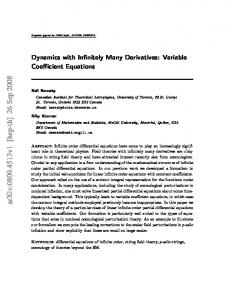
presented in Section VI. Notation: The set B c denotes the complement of a set B. Notation PB and EB denotes the probability measure and expectation under a distribution PB . The ij-th entry of a matrix A is denoted by [A]ij or aij . Random variables are denoted with upper-case letters, while the corresponding lower-case letters denote their realizations. Time indices are indicated by subscripts and the letter k. Superscripts represent the agent indices, which are usually i or j. II. P ROBLEM F ORMULATION We consider the problem of distributed non-Bayesian learning, where a network of agents access sequences of realizations of a random variable with an unknown distribution. The random variable is assumed to be of finite dimension with the constraint that each agent can access only a strict subset of the entries of the realizations (e.g., an n-dimensional vector and n agents each observing a single entry). Observations are assumed to be independent among the agents. We are interested in situations where no single agent has the ability to learn the underlying distribution from its own observations, while collectively the agents can do so if they collaborate. The learning objective is for the agents to jointly agree on a distribution (from a parametrized family of distributions or a hypothesis set) that best describes the observations in a specific sense (e.g., Kullback-Leibler divergence). Therefore, the distributed learning objective requires collaboration among the agents which can be ensured by using some protocols for information aggregation and coordination. Specifically in our case, agent coordination consists of sharing their estimates (beliefs) of the best probability distribution over the hypothesis set. Consider, for example, the distributed source location problem with limited sensing capabilities [25], [26]. In this scenario a network of n agents receives noisy measurements of the distance to a source, where sensing capabilities of each sensor might be limited to a certain region. The group objective is to jointly identify the location of the source and that every node knows the source location. Figure 1 shows an example, where a group of 7 agents (circles) wants to localize a source (star). There is an underlying graph that indicates the communication abilities among the nodes. Moreover, each node has a sensing region indicated by the dashed line around it. Each agent i obtains realizations of the random variable Ski = kxi − θ∗ k + Wki , where θ∗ is the

location of the source, xi is the position of agent i and Wki is a noise in the observations. If

we consider Θ as the set of all possible locations of the source, then each θ ∈ Θ will induce a May 10, 2016

DRAFT

4

probability distribution about the observations of each agent. Therefore, agents need to cooperate and share information in order to guarantee that all of them correctly localize the target.

Fig. 1: Distributed source localization example

We will consider a more general learning problem, where agent observations are drawn from an Q unknown joint distribution f = ni=1 f i , where f i is the distribution governing the observations Q of agent i. We assume that f is an element of P = ni=1 P i , the space of all joint probability measures for a set of n independent random variables {S i }ni=1 (i.e., S i is distributed according

to an unknown distribution f i ). Also, we assume that each S i takes values in a finite set. When these random variables are considered at time k, we denote them by Ski . Later on, for the case of countably many hypotheses, we will use the pre-metric space (P, DKL ) as the vector space P equipped with the Kullback-Liebler divergence. This will generate a topology, where we can define an open ball Br (p) with a radius r > 0 centered at a point p ∈ P by Br (p) = {q ∈ P|DKL (q, p) < r}. When the set of hypothesis is continuous, we instead equip P with the Hellinger distance h to obtain the metric space (P, h), which we use to construct a special covering of subsets B ⊂ P consisting of δ-separated sets.

Each agent constructs a set of hypothesis parametrized by θ ∈ Θ about the distribution f i .

Let L i = {Pθi |θ ∈ Θ} be a parametrized family of probability measures for Ski with densities ℓi (·|θ) = dPθi /dλi with respect to a dominating measure1 λi . Therefore, the learning goal is to 1

A measure µ is dominated by λ if λ(B) = 0 implies µ(B) = 0 for every measurable set B.

May 10, 2016

DRAFT

5

distributively solve the following problem: min F (θ) , DKL (f kℓ (·|θ))

(1)

θ∈Θ

=

n X i=1

where ℓ (·|θ) =

Qn

i=1

DKL f i kℓi (·|θ)




ℓi (·|θ) and DKL (f i kℓi (·|θ)) is the Kullback-Leibler divergence between

the true distribution of Ski and ℓi (·|θ) that would have been seen by agents i if hypothesis θ were correct. For simplicity we will assume that there exists a single θ∗ ∈ Θ such that ℓi (·|θ∗ ) = f i

almost everywhere for all agents. Results readily extends to the case when the assumption does not hold (see, for example, [27], [20], [22] which disregard this assumption). The problem in Eq. (1) consists of finding the parameter θ∗ such that ℓ (·|θ) =

Qn

i=1

ℓi (·|θ)

minimizes its Kullback-Liebler divergence to f . However, L i is only available to agent i and the distribution f is unknown. Agent i gains information on f i by observing realizations sik of Ski at every time step k. The agent uses these observations to construct a sequence {µik } of probability distributions over the parameter space Θ. We refer to these distributions as agent i beliefs, where µik (B) denotes the belief, at time k, that agent i has about the event θ∗ ∈ B ⊆ Θ for a measurable set B. We make use of the following assumption. Assumption 1 For all agents i = 1, . . . , n we have: (a) There is a unique hypothesis θ∗ such that ℓi (·|θ∗ ) = f i . (b) If f i (si ) > 0, then there exists an α > 0 such that ℓi (si |θ) > α for all θ ∈ Θ. Assumption 1(a) guarantees that we are working on the realizable case and there are no conflicting models among the agents, see [27], [20], [22] for ways of how to remove this assumption. Moreover in Assumption 1(b), the lower bound α assumes the set of hypothesis are dominated by f i (i.e., our hypothesis set is absolutely continuous with respect to the true distribution of the data) and provide a way to show bounded differences when applying the concentration inequality results. Agents are connected in a network G = {V, E} where V = {1, 2, . . . , n} is the set of agents and E is a set of undirected edges, where (i, j) ∈ E if agents i and j can communicate with each other. If two agents are connected they share their beliefs over the hypothesis set at every time May 10, 2016

DRAFT

6

instant k. We will propose a distributed protocol to define how the agents update their beliefs based on their local observations and the beliefs received from their neighbors. Additionally, each agent weights its own belief and the beliefs of its neighbors; we will use aij to denote the weight that agent i assigns to beliefs coming from its neighbor j, and aii to denote the weight that the agent assigns to its own beliefs. The assumption of static undirected links in the network is made for simplicity of the exposition. The extensions of the proposed protocol to more general cases of time varying undirected and directed graphs can be done similar to the work in [27], [20], [22]. Next we present the set of assumptions on the network over which the agents are interacting.

Assumption 2 The graph G and matrix A are such that: (a) A is doubly-stochastic with [A]ij = aij > 0 if (i, j) ∈ E. (b) If (i, j) ∈ / E for some i 6= j then aij = 0.

(c) A has positive diagonal entries, aii > 0 for all i ∈ V .

(d) If aij > 0, then aij ≥ η for some positive constant η. (e) The graph G is connected.

Assumption 2 is common in distributed optimization and consensus literature. It guarantees convergence of the associated Markov Chain and defines bounds on relevant eigenvalues in terms of the number n of agents. To construct a set of weights satisfying Assumptions 2, for example, one can consider a lazy metropolis (stochastic) matrix of the form A¯ = 1 I + 1 A, where 2

2

I is the identity matrix and A is a stochastic matrix whose off-diagonal entries satisfy  1  if (i, j) ∈ E max{di +1,dj +1} aij =  0 if (i, j) ∈ /E

where di is the degree (the number of neighbors) of node i. Generalizations of Assumption 2 to time-varying undirected are readily available for weighted averaging and push-sum approaches [28], [10], [9]. III. D ISTRIBUTED L EARNING A LGORITHM In this section, we present the proposed learning algorithm and a novel connection between Bayesian update and the stochastic mirror descent method. We propose the following (theoretical) May 10, 2016

DRAFT

7

algorithm, where each node updates its beliefs on a measurable subset B ⊆ Θ according to the following update rule: for all agents i and all k ≥ 1, !aij Z Y n j dµ (θ) 1 k−1 ℓi (sik |θ)dλ (θ) µik (B) = i Zk dλ(θ) j=1

(2)

θ∈B

where

Zki

is a normalizing constant and λ is a probability distribution on Θ with respect to which

every µjk is absolutely continuous. The term dµjk (θ)/dλ(θ) is the Radon-Nikodym derivative of the probability distribution µjk . The above process starts with some initial beliefs µi0 , i = 1, . . . , n. Note that, if Θ is a finite or a countable set, the update rule in Eq. (2) reduces to: for every B ⊆ Θ, µik

n
1 XY j (B) = i µk−1 (θ)aij ℓi sik |θ Zk j=1

(3)

θ∈B

The updates in Eqs. (2) and (3) can be viewed as two-step processes. First, every agent constructs an aggregate belief using weighted geometric average of its own belief and the beliefs of its neighbors. Then, each agent performs a Bayes’ update using the aggregated belief as a prior. A. Connection with the Stochastic Mirror Descent Method To make this connection2, we observe that the optimization problem in Eq. (1) is equivalent to the following problem: min Eπ

π∈PΘ

n X i=1

i

DKL f kℓ

i




= min

π∈PΘ

n X

Eπ Ef i [− log ℓi ]

i=1

where PΘ is the set of all distributions on Θ. Under some technical conditions the expectations can exchange the order, so the problem in Eq. (1) is equivalent to the following one: min

π∈PΘ

n X

Ef i Eπ [− log ℓi ]

(4)

i=1

The difficulty in evaluating the objective function in Eq. (4) lies in the fact that the distributions f i are unknown. A generic approach to solving such problems is the class of stochastic approximation methods, where the objective is minimized by constructing a sequence of gradient-based iterates where the true gradient of the objective (which is not available) is replaced with a gradient sample that is available at the given update time. A particular method that is relevant 2

Particularly simple when Θ is a finite set.

May 10, 2016

DRAFT

8

here is the stochastic mirror-descent method which would solve the problem in Eq. (4), in a centralized fashion, by constructing a sequence {xk }, as follows:   1 Dw (y, xk−1) xk = arg min hgk−1 , yi + αk−1 y∈X

(5)

where gk is a noisy realization of the gradient of the objective function in Eq. (4) and Dw (y, x) is a Bregman distance function associated with a distance-generating function w, and αk > 0 is the step-size. If we take w(t) = t log t as the distance-generating function, then the corresponding Bregman distance is the Kullback-Leiblier (KL) divergence DKL . Thus, in this case, the update rule in Eq. (2) corresponds to a distributed implementation of the stochastic mirror descent algorithm in (5), where Dw (y, x) = DKL (y, x) and the stepsize is fixed, i.e.., αk = 1 for all k. We summarize the preceding discussion in the following proposition. Proposition 1 The update rule in Eq. (2) defines a probability measure µik over the set Θ generated by the probability density µ ¯ik = dµik /dλ that coincides with the solution of the distributed stochastic mirror descent algorithm applied to the optimization problem in Eq. (1)., i.e. (

µ ¯ ik = arg min Eπ [– log ℓi (sik |·)] + π∈PΘ

n X

aij DKL (πk¯ µjk−1)

j=1

)

(6)

Proof: We need to show that the density µ ¯ ik associated with the probability measure µik defined by Eq. (2) minimizes the problem in Eq. (6). First, define the argument in Eq. (6) as G(π) = −Eπ log ℓ

i

sik |·




+

n X

aij DKL π||¯ µjk−1

j=1




and add and subtract the KL divergence between π and the density µ ¯ ik to obtain G(π) = −Eπ log ℓ

i

(sik |·)

+

n X j=1

aij DKL (πk¯ µjk−1) − DKL (πkµik ) + DKL (πk¯ µik )

= −Eπ log ℓi sik |· + DKL πk¯ µk +


= −Eπ log ℓ

May 10, 2016

i

(sik |·)

+


i

DKL πk¯ µik




+

n X

aij Eπ

log

j=1

n X j=1

aij Eπ log

π µ ¯jk−1

π − log i µ ¯k

!

µ ¯ik µ ¯jk−1

DRAFT

9

Now, we use the relation for the density µ ¯ik = dµik /dλ, which is implied by the update rule for µik in Eq. (2), and obtain
i

G(π) = −Eπ log ℓi sik |· + DKL πk¯ µk +


= − log Zki + DKL πk¯ µik

n X

aij Eπ log

j=1

n 1 Y m
aim i i µ ¯k−1 ℓ (sk |·) µ ¯jk−1 Zki m=1

1

!




The first term in the preceding line does not depend on the distribution π. Thus, we conclude that the solution to the problem in Eq. (6) is the density π ∗ = µ ¯ik (almost everywhere). IV. C OUNTABLE H YPOTHESIS S ET In this section we present a concentration result for the update rule in Eq. (3) specific for the case of a countable hypothesis set. Later in Section V we will analyze the case of Θ ⊂ Rd . First, we provide some definitions that will help us build the desired results. Specifically, we will study how the beliefs of all agents concentrate around the true hypothesis θ∗ . Definition 1 Define a Kullback-Leibler Ball (KL) of radius r centered at θ∗ as. ) ( n 1 X
DKL ℓi (·|θ∗ ) , ℓi (·|θ) ≤ r Br (θ∗ ) = θ ∈ Θ n i=1

Definition 2 Define the covering of the set Brc (θ∗ ) generated by a strictly increasing sequence

{rl }∞ l=1 with r1 = r as the union of disjoint KL bands as follows: Brc (θ∗ )

=

∞ [

{Brl+1 (θ∗ )\Brl (θ∗ )}

l=1

where {Brl+1 \Brl } denotes the complement between the set Brl+1 and the set Brl+1 , i.e. Brl+1 ∩Brcl We denote the cardinality {Br \Br } by Nr , i.e. {Br \Br } = Nr . l+1

l

l

l+1

l

l

We are interested in bounding the beliefs’ concentration on a ball Br (θ∗ ) for an arbitrary r > 0,

which is based on a covering of the complement set Brc (θ∗ ). To this end, Definitions 1 and 2

provide the tools for constructing such a covering. The strategy is to analyze how the hypotheses are distributed in the space of probability distributions, see Figure 2. The next assumption will provide conditions on the hypothesis set which guarantee the concentration results. Assumption 3 The series Σl≥1 exp (−rl2 + log Nrl ) converges, where the sequence {rl } is as in Definition 2. May 10, 2016

DRAFT

10

Pθ

Pθ∗ Br (θ∗ ) Br2 (θ∗ )

Fig. 2: Creating a covering for a ball Br (θ∗ ). ⋆ represents the correct hypothesis ℓi (·|θ∗ ), • indicates the location of other hypotheses and the dash lines indicates the boundary of the balls Brl (θ∗ ).

We are now ready to state the main result for a countable hypothesis set Θ. Theorem 1 Let Assumptions 1, 2 and 3 hold, and let ρ ∈ (0, 1) be a desired probability

tolerance. Then, the belief sequences {µik }, i ∈ V , generated by the update rule in Eq. (3), with

the initial beliefs such that µi0 (θ∗ ) > ǫ for all i, have the following property: for any σ ∈ (0, 1) and any radius r > 0 with probability 1 − ρ, µik (Br (θ∗ )) ≥ 1 − σ

for all i and all k ≥ N

where N = mink≥1 {k ∈ N1 ∩ N2 } with the sets N1 and N2 given by ! ) ( X
1 Nr exp −krl2 ≤ ρ N1 = k | exp 8 log2 α1 l≥1 l ( )   n Y 1 k N2 = k | C3 exp − γ(θ) ≤ σ µi0 (θ) n , ∀θ 6∈ Br (θ∗ ) 2 i=1   1 P log n 8 log α , α is as in Assumpwhere γ(θ) = n1 ni=1 DKL (ℓi (·|θ∗ ) ||ℓi (·|θ)), C3 = 1ǫ exp 1−λ

tion 1(b), Nrl and rl are as in Definition 2, while λ = 1 − η/4n2 . If A is a lazy-metropolis

matrix, then λ = 1 − 1/O(n2 ).

May 10, 2016

DRAFT

11

Observe that if k ∈ N1 , then m ∈ N1 for all m ≥ k, and the same is true for the set N2 , so we can alternatively write 



N = max min{k ∈ N1 }, min{k ∈ N2 } . k≥1

k≥1

Further, note that N depends on the radius r of the KL ball, as the set N1 involves Nrl and rl which both depend on r, while the set N2 explicitly involves r. Finally, note that the smaller the radius r, the larger N is. We see that N also depends on the number n of agents, the learning parameter α, the learning capabilities of the network represented by γ(θ), the initial beliefs µi0 , the number of hypotheses that are far away from θ∗ and their probability distributions. Theorem 1 states that the beliefs of all agents will concentrate within the KL ball Br (θ∗ ) with a radius r > 0 for a large enough k, i.e., k ≥ N. Note that the (large enough) index N is determined as the smallest k for which two relations are satisfied, namely, the relations defining the index sets N1 and N2 . The set N1 contains all indices k for which a weighted sum of the total mass of the hypotheses θ ∈ / Br (θ∗ ) is small enough (smaller than the desired probability tolerance ρ). Specifically, we require the number Nrl of hypothesis in the l-th band

does not grow faster than the squared radius rl2 of the band, i.e., the wrong hypothesis should not accumulate too fast far away from the true hypothesis θ∗ . Moreover, the condition in N1 also prevents having an infinite number of hypothesis per band. The set N2 captures the iterations k at which, for all agents, the current beliefs µik had recovered from the the cumulative effect of “wrong” initial beliefs that had given probability masses to hypotheses far away from θ∗ . In the proof for Theorem 1, we use the relation between the posterior beliefs and the initial beliefs on a measurable set B such that θ∗ ∈ B. For such a set, we have µik (B) =

n k n 1 XY j [Ak ]ij Y Y ℓj (sj |θ)[Ak−t ]ij µ (θ) t 0 Zki t=1 j=1 j=1

(7)

θ∈B

where

Zki

is the appropriate normalization constant. Furthermore, after a few algebraic operations

we obtain µik

(B) ≥ 1–

n XY

θ∈B c j=1

µj0 (θ) µj0 (θ∗ )

![Ak ]

ij

k Y n Y t=1 j=1

ℓj (sjt |θ) ℓj (sjt |θ∗ )

![Ak-t ]

ij

(8)

Moreover, since µj0 (θ∗ ) > ǫ for all j, it follows that n k 1 X YY i µk (B) ≥ 1– ǫ c t=1 j=1 θ∈B

May 10, 2016

ℓj (sjt |θ) ℓj (sjt |θ∗ )

![Ak-t ] ij

(9)

DRAFT

12

Now we will state a useful result from [19] which will allow us to bound the right hand term of Eq. (8). Lemma 1 [Lemma 2 in [19]] Let Assumptions 2 hold, then the matrix A satisfies: for all i, k X n X 4 log n  k−t  1 ≤ A − ij n 1−λ t=1 j=1

where λ = 1 − η/4n2 , and if A is a lazy-metropolis matrix associated with G then λ = 1 −

1/O(n2 ).

If follows from Eq. (9), Lemma 1 and Assumption 1 that µik (B) ≥ 1–C3

k Y n XY

θ∈B c t=1 j=1

ℓj (sjt |θ) ℓj (sjt |θ∗ )

! n1

(10)

for all i, where C3 is as defined in Theorem 1. Next we provide an auxiliary result about the concentration properties of the beliefs on a set B. Lemma 2 For any k ≥ 0 it holds that ! X [ 
k Nrl exp −krl2 ≤ C2 v¯k (θ) ≥ − γ(θ) Pf 2 l≥1 θ∈B c   where C2 = exp 18 log12 1 , γ(θ) and Nrl and rl are as in Theorem 1. α

Proof: First define the following random variable

k n X 1X ℓi (S i |θ) v¯k (θ) = log i it ∗ n i=1 ℓ (St |θ ) t=1

Then, by using the union bound and McDiarmid inequality we have, ! X [ Pf {¯ vk (θ) − Ef v¯k (θ) ≥ ¯ǫ} {¯ vk (θ)-Ef v¯k (θ) ≥ ǫ¯} ≤ Pf θ∈B c

θ∈B c

≤

X

θ∈B c

2

exp

2¯ǫ 4k log2

and by setting ǫ = − 12 Ef [¯ vk (θ)], it follows that ! X [  1 exp vk (θ)] ≤ v¯k (θ) ≥ Ef [¯ Pf 2 c c θ∈B θ∈B May 10, 2016

1 α

!

(Ef [¯ vk (θ)])2 8k log2 α1

! DRAFT

13

It can be seen that Ef [¯ vk (θ)] = −kγ(θ), thus yielding ! X [ 
k ≤ C2 exp −kγ 2 (θ) Pf v¯k (θ) ≥ − γ(θ) 2 c c θ∈B

θ∈B

Now, we let the set B be the KL ball of a radius r centered at θ∗ and follow Definition 2 to exploit the representation of Brc (θ∗ ) as the union of KL bands, for which we obtain X
X X
exp −kγ 2 (θ) = exp −kγ 2 (θ) θ∈Brc (θ ∗ )

l≥1 θ∈Brl+1 \Brl

≤

X l≥1

Nrl exp −krl2

thus, completing the proof.




We are now ready to proof Theorem 1 Theorem 1: From Lemma 2, where we take k large enough to ensure the desired probability, it follows that with probability 1 − ρ, we have: for all k ∈ N1 ,   X k i ∗ µk (Br (θ )) ≥ 1 − C3 exp − γ(θ) 2 c ∗ θ∈Br (θ )

≥1−

X

θ∈Brc (θ ∗ )

σ

n Y

1

µi0 (θ) n

i=1

≥1−σ where the last inequality follows from Eq. (10) where we further take sufficiently large k. V. C ONTINUUM

OF

H YPOTHESES

In this section we will provide the concentration results for a continuous hypothesis set Θ ⊆

Rd . At first, we present some definitions that we use in constructing coverings analogously to that in Section IV. In this case, however, we employ the Hellinger distance. Definition 3 Define a Hellinger Ball (H) of radius r centered at θ∗ as.   1 ∗ ∗ Br (θ ) = θ ∈ Θ √ h (ℓ (·|θ ) , ℓ (·|θ)) ≤ r n

Definition 4 Let (M, d) be a metric space. A subset Sδ ⊆ M is called δ-separated with δ > 0 if d(x, y) ≥ δ for any x, y ∈ Sδ . Moreover, for a set B ⊆ M, let NB (δ) be the smallest number

May 10, 2016

DRAFT

14

of Hellinger balls with centers in Sδ of radius δ > 0 needed to cover the set B, i.e., such that S B ⊆ z∈Sδ Bδ (z).

Definition 5 Let {rl } be a strictly decreasing sequence such that r1 = 1 and liml→∞ rl = 0. Define the covering of the set Brc (θ∗ ) generated by the sequence {rl } as follows: Brc (θ∗ )

=

L[ r −1 l=1

{Brl \Brl+1 }

where Lr is the smallest l such that rl ≤ r. Moreover, given a positive sequence {δl }, we denote by Nrl (δl ) the maximal δl -separated subset of the set {Brl \Brl+1 } and denote its cardinality by

Kl , i.e. Kl = |Nl (δl )|. Therefore, we have the following covering of Brc (θ∗ ), Brc (θ∗ ) =

L[ r −1

[

l≥1 zm ∈Nl (δl )

Fl,m

where Fl,m = Bδl (zm ∈ Nrl (δl )) ∩ {Brl \Brl+1 }. Figure 3 depicts the elements of a covering for a set Brc (θ∗ ). The cluster of circles at the top right corner represents the balls Bδl (zm ∈ Nrl (δl )) and for a specific case in the left of the image we illustrate the set Fl,m.

Fl,m

Pθ∗

Br (θ∗ )

Fig. 3: Creating a covering for a set Br (θ∗ ). ⋆ represents the correct hypothesis ℓi (·|θ∗ ). We are now ready to state the main result regarding continuous set of hypotheses Θ ⊆ Rd .

May 10, 2016

DRAFT

15

Theorem 2 Let Assumptions 1, 2, and 3 hold, and let ρ ∈ (0, 1) be a given probability tolerance

level. Then, the beliefs {µik }, i ∈ V, generated by the update rule in Eq. (2) with uniform initial

beliefs, are such that, for any σ ∈ (0, 1) and any r > 0 with probability 1 − ρ, µik (Br (θ∗ )) ≥ 1 − σ

for all i and all k ≥ N

where N = min {k ≥ 1 |k ∈ N1 and k ∈ N2 } with ) (L −1   r X 8 log α1 log n exp –k (rl+1 –δl –R) –d log δl ≤ ρ N1 = 1−λ l=1 (L −1 ) r   X rl exp d log − 2k (rl+1 − δl − R) ≤ σ N2 = R l=1

for a parameter R such that r > R and rl+1 − δl − R > 0 for all l ≥ 1. The constant α is as

in Assumption 1, d is the dimension of the space of Θ, rl and δl are as in Definition 5, while λ is the same as in Theorem 1. Analogous to Theorem 1, Theorem 2 provides a probabilistic concentration result for the agents’ beliefs around a Hellinger ball of radius r with center at θ∗ for sufficiently large k. Similarly to the preceding section, we represent the beliefs µik in terms of the initial beliefs and the cumulative product of the weighted likelihoods received from the neighbors. In particular, analogous to Eq. (7), we have that for every i and for every measurable set B ⊆ Θ: Z Y k Y n 1 Ak−t ] j i ij dµ (θ) µk (B) = i ℓj (sjt |θ)[ 0 Zk t=1 j=1

(11)

θ∈B

with the corresponding normalization constant Zki , and assuming all agents have uniform beliefs at time 0. It will be easier to work with the beliefs’ densities, so we define the density of a measurable set with respect to the observed data. Definition 6 The density gBi of a measurable set B ⊆ Θ, where µi0 (B) > 0 with respect to the product distribution of the observed data is given by Z Y k Y n 1 At−k ] j i ij dµ (θ) ℓj (Stj |θ)[ gB (ˆ s) = i 0 µ0 (B) t=1 j=1

(12)

B

where sˆ =

May 10, 2016

i=1:n {Sti }t=1:k

and

PBi

=

gBi

i ⊗k

· (λ ) . DRAFT

16

The next lemma relates the density gBi (ˆ s) which is defined per agent to a quantity that is common among all nodes in the network. Lemma 3 Consider the densities as defined in Eq. (12), then 1

gBi (ˆ s) ≤ C1 gB (ˆ s) n where C1 = exp



1 8 log α log n 1−λ



(13)

and gB (ˆ s) =

Z Y k Y n B

t=1 j=1

ℓj (Stj |θ)dµj0 (θ) .

Proof: By definition of the densities, we have Z Y k Y n 1 [At−k ]ij j i gB (ˆ s) = i dµ0 (θ) ℓj (Stj |θ) µ0 (B) t=1 j=1 B

1 = i µ0 (B)

Z

1 = i µ0 (B)

Z

exp

t=1 j=1

B

B

k X n X 

exp

!  At−k ij log ℓj (Stj |θ) dµj0 (θ)

k X n  X  t=1 j=1

 1 At−k ij − n



! n k X X 1 j log ℓj (Sti |θ) + log ℓj (St |θ) dµj0 (θ) n j=1 t=1

where the last line follows by adding and subtracting 1/n. Hence, by Lemma 1, we further obtain C1 gBi (ˆ s) ≤ i µ0 (B) =

≤

C1 i µ0 (B) C1 (B)

µi0

Z

B

! n k X 1X exp log ℓj (Stj |θ) dµj0 (θ) n j=1 t=1

Z Y k Y n

B

t=1 j=1

ℓj (Stj |θ)1/n dµj0 (θ)

 1/n Z Y n k Y  ℓj (Stj |θ)dµj0 (θ) B

t=1 j=1

where the last inequality follows from Jensen’s inequality.

The next Lemma is an analog of Lemma 2 which we use to bound the probability concentrations with respect to the ratio gFi l,m (ˆ s) /gBi R (θ∗ ) (ˆ s). Lemma 4 Consider the ratio gFi l,m (ˆ s) /gBi R (θ∗ ) (ˆ s), then ! ! gFi l,m (ˆ s) ≥ −2k (rl − δl − R) ≤ C2 exp (−k (rl+1 − δl − R) + d log δl ) . PBR (θ∗ ) log gBi R (θ∗ ) (ˆ s) May 10, 2016

DRAFT

17

with C2 as defined in Lemma 2. Proof: By using the union bound, the Markov inequality and Lemma 1 in [24], we have that PBR (θ∗ ) log

gFi l,m (ˆ s) gBi R (θ∗ ) (ˆ s)

!

≥y

!

   y 1 2 ∗ ≤ C1 exp − exp −k h (Fl,m, BR (θ )) 2 n   y ≤ C1 exp − − 2k (rl+1 − δl − R) 2

where the last inequality follows from Proposition 5 and Corollary 1 in [24], where 1 1 √ h (Fl,m , BR (θ∗ )) ≥ √ h (zm ∈ Nrl (δl ) , θ∗ ) − δl − R n n ≥ (rl+1 − δl − R) The desired result is obtained by letting y = −2k (rl+1 − δl − R). Furthermore,  PBR (θ∗ ) 

[

Fl,m

(

log

gFi l,m (ˆ s) i gBR (θ∗ ) (ˆ s)

!

)

≥y ≤

Kl L r −1 X X

PBR (θ∗ ) log

l=1 m=1

≤ C2 ≤ C2

L r −1 X l=1

L r −1 X l=1

gFi l,m (ˆ s) gBi R (θ∗ ) (ˆ s)

!

≥y

!

Kl exp (−k (rl+1 − δl − R)) exp (−k (rl+1 − δl − R) − d log δl )

where the last inequality follows from Kl ≥ δl−d , see [30], [31].

Lemma 3 allows us to represent the beliefs on the set B c as the cumulative beliefs with

respect to the density gB (ˆ s). For this, similarly as in Section IV we will partition the set B c into Hellinger bands. Then for each band we will find a covering of δ-separated balls and compute the concentration of probability measure with respect to density rations. Proof: [Theorem 2] Lets consider the Hellinger ball Br (θ∗ ). We thus have µik (Br (θ∗ )) =

R

θ∈Br

(θ ∗ )

R

k Q n Q

t=1 j=1

k Q

n Q

θ∈Θ t=1 j=1

May 10, 2016

ℓj (sjt |θ)

ℓj (sjt |θ)

[Ak−t ]ij

[Ak−t ]ij

dµj0 (θ)

dµj0 (θ)

DRAFT

18

≥1−

R

θ∈Brc (θ ∗ )

t=1 j=1

R

k Q n Q

θ∈BR

≥1−

k Q n Q

R

(θ ∗ )

ℓj (sjt |θ)

t=1 j=1 k Q n Q

θ∈Brc (θ ∗ ) t=1 j=1

[Ak−t ]ij

dµj0 (θ)

[Ak−t ]ij

dµj0 (θ)

ℓj (sjt |θ)

ℓj (sjt |θ)[

Ak−t ]

ij

dµj0 (θ) (14)

µi0 (BR (θ∗ )) gBi R (θ∗ ) (ˆ s)

The construction of a partition of the set Brc presented in Definition 5 allows us to rewrite Eq. (14) as follows:

µik (Brc (θ∗ )) ≤ =

Kl LP r −1 P

k Q n R Q

l=1 m=1 Fl,m t=1 j=1

ℓj (sjt |θ)[

Ak−t ]

ij

dµj0 (θ)

µi0 (BR (θ∗ )) gBi R (θ∗ ) (ˆ s)

Kl LX r −1 X l=1

i s) µj0 (Fl,m ) gFl,m (ˆ i i µ (BR (θ∗ )) gBR (θ∗ ) (ˆ s) m=1 0

Finally by applying Lemma 4 and the fact that of all agents have uniform initial beliefs Kl L r −1 X X

µj0 (Fl,m) exp(−2k (rl+1 -δl -R)) j ∗ )) µ (B (θ R l=1 m=1 0
L r −1 X µj0 Brl+1 (θ∗ ) ≤ exp(−2k (rl+1 − δl − R)) µj0 (BR (θ∗ )) l=1

µik (Brc (θ∗ )) ≤

≤

L r −1 X l=1

  rl+1 exp d log − 2k (rl+1 − δl − R) R

The last inequality follows from the initial beliefs being uniform and the volume ratio of the two Hellinger balls with radius rl and R. VI. C ONCLUSIONS We proposed an algorithm for distributed learning with a countable and a continuous sets of hypotheses. Our results show non-asymptotic geometric convergence rates for the concentration of the beliefs around the true hypothesis. While the proposed algorithm is motivated by the non-Bayesian learning models, we have shown that it is also a specific instance of a distributed stochastic mirror descent applied to a well defined optimization problem consisting of the minimization of the sum of KullbackLiebler divergences. This indicates an interesting connection between two “separate” streams of May 10, 2016

DRAFT

19

literature and provides an initial step to the study of distributed algorithms in a more general form. Specifically, it is interesting to explore how variations on stochastic approximation algorithms will induce new non-Bayesian update rules for more general problems. In particular, one would be interested in acceleration results for proximal methods, other Bregman distances and other constraints in the space of probability distributions. Interaction between the agents is modeled as exchange of local probability distributions (beliefs) over the hypothesis set between connected nodes in a graph. This will in general generate high communication loads. Nevertheless, results are an initial study towards the distributed learning problems for general hypothesis sets. Future work will consider the effect of parametric approximation of the beliefs such that one only needs to communicate a finite number of parameters such as, for example, in Gaussian Mixture Models or Particle Filters. R EFERENCES [1] V. C. Gungor, B. Lu, and G. P. Hancke, “Opportunities and challenges of wireless sensor networks in smart grid,” IEEE Transactions on Industrial Electronics, vol. 57, no. 10, pp. 3557–3564, 2010. [2] A. Mainwaring, D. Culler, J. Polastre, R. Szewczyk, and J. Anderson, “Wireless sensor networks for habitat monitoring,” in Proceedings of the 1st ACM international workshop on Wireless sensor networks and applications.

ACM, 2002, pp.

88–97. [3] C.-Y. Chong and S. P. Kumar, “Sensor networks: evolution, opportunities, and challenges,” Proceedings of the IEEE, vol. 91, no. 8, pp. 1247–1256, 2003. [4] A. Jadbabaie, P. Molavi, A. Sandroni, and A. Tahbaz-Salehi, “Non-bayesian social learning,” Games and Economic Behavior, vol. 76, no. 1, pp. 210–225, 2012. [5] P. Molavi, A. Tahbaz-Salehi, and A. Jadbabaie, “Foundations of non-bayesian social learning,” Columbia Business School Research Paper, 2015. [6] D. Acemoglu, A. Nedi´c, and A. Ozdaglar, “Convergence of rule-of-thumb learning rules in social networks,” in Proceedings of the IEEE Conference on Decision and Control, 2008, pp. 1714–1720. [7] J. N. Tsitsiklis and M. Athans, “Convergence and asymptotic agreement in distributed decision problems,” IEEE Transactions on Automatic Control, vol. 29, no. 1, pp. 42–50, 1984. [8] A. Jadbabaie, J. Lin, and A. S. Morse, “Coordination of groups of mobile autonomous agents using nearest neighbor rules,” IEEE Transactions on Automatic Control, vol. 48, no. 6, pp. 988–1001, 2003. [9] A. Nedi´c and A. Olshevsky, “Distributed optimization over time-varying directed graphs,” IEEE Transactions on Automatic Control, vol. 60, no. 3, pp. 601–615, 2015. [10] A. Olshevsky, “Linear time average consensus on fixed graphs and implications for decentralized optimization and multiagent control,” preprint arXiv:1411.4186, 2014. [11] D. Acemoglu, M. A. Dahleh, I. Lobel, and A. Ozdaglar, “Bayesian learning in social networks,” The Review of Economic Studies, vol. 78, no. 4, pp. 1201–1236, 2011.

May 10, 2016

DRAFT

20

[12] E. Mossel, A. Sly, and O. Tamuz, “Asymptotic learning on bayesian social networks,” Probability Theory and Related Fields, vol. 158, no. 1-2, pp. 127–157, 2014. [13] S. Shahrampour and A. Jadbabaie, “Exponentially fast parameter estimation in networks using distributed dual averagingy,” in Proceedings of the IEEE Conference on Decision and Control, 2013, pp. 6196–6201. [14] A. Lalitha, A. Sarwate, and T. Javidi, “Social learning and distributed hypothesis testing,” in IEEE International Symposium on Information Theory, 2014, pp. 551–555. [15] L. Qipeng, F. Aili, W. Lin, and W. Xiaofan, “Non-bayesian learning in social networks with time-varying weights,” in 30th Chinese Control Conference (CCC), 2011, pp. 4768–4771. [16] L. Qipeng, Z. Jiuhua, and W. Xiaofan, “Distributed detection via bayesian updates and consensus,” in 34th Chinese Control Conference, 2015, pp. 6992–6997. [17] S. Shahrampour, M. Rahimian, and A. Jadbabaie, “Switching to learn,” in Proceedings of the American Control Conference, 2015, pp. 2918–2923. [18] M. A. Rahimian, S. Shahrampour, and A. Jadbabaie, “Learning without recall by random walks on directed graphs,” preprint arXiv:1509.04332, 2015. [19] S. Shahrampour, A. Rakhlin, and A. Jadbabaie, “Distributed detection: Finite-time analysis and impact of network topology,” IEEE Transactions on Automatic Control, vol. PP, no. 99, pp. 1–1, 2015. [20] A. Nedi´c, A. Olshevsky, and C. A. Uribe, “Fast convergence rates for distributed non-bayesian learning,” preprint arXiv:1508.05161, Aug. 2015. [21] A. Lalitha, T. Javidi, and A. Sarwate, “Social learning and distributed hypothesis testing,” preprint arXiv:1410.4307, 2015. [22] A. Nedi´c, A. Olshevsky, and C. A. Uribe, “Network independent rates in distributed learning,” preprint arXiv: 1509.08574, 2015. [23] L. Su and N. H. Vaidya, “Asynchronous distributed hypothesis testing in the presence of crash failures,” University of Illinois at Urbana-Champaign, Tech. Rep., 2016. [24] L. Birg´e, “About the non-asymptotic behaviour of bayes estimators,” Journal of Statistical Planning and Inference, vol. 166, pp. 67–77, 2015. [25] M. Rabbat and R. Nowak, “Decentralized source localization and tracking wireless sensor networks,” in Proceedings of the IEEE International Conference on Acoustics, Speech, and Signal Processing, vol. 3, 2004, pp. 921–924. [26] M. Rabbat, R. Nowak, and J. Bucklew, “Robust decentralized source localization via averaging,” in IEEE International Conference on Acoustics, Speech, and Signal Processing., vol. 5, 2005, pp. 1057–1060. [27] A. Nedi´c, A. Olshevsky, and C. A. Uribe, “Nonasymptotic convergence rates for cooperative learning over time-varying directed graphs,” in Proceedings of the American Control Conference, 2015, pp. 5884–5889. [28] A. Nedi´c, A. Olshevsky, A. Ozdaglar, and J. N. Tsitsiklis, “On distributed averaging algorithms and quantization effects,” IEEE Transactions on Automatic Control, vol. 54, no. 11, pp. 2506–2517, 2009. [29] L. Birg´e, “Model selection via testing: an alternative to (penalized) maximum likelihood estimators,” Annales de l’Institut Henri Poincare (B) Probability and Statistics, vol. 42, no. 3, pp. 273 – 325, 2006. [30] I. Dumer, “Covering spheres with spheres,” Discrete & Computational Geometry, vol. 38, no. 4, pp. 665–679, 2007. [31] C. Rogers, “A note on coverings,” Mathematika, vol. 4, no. 01, pp. 1–6, 1957.

May 10, 2016

DRAFT