DISTRIBUTED-MEMORY PARALLEL ALGORITHMS FOR DISTANCE

DISTRIBUTED-MEMORY PARALLEL ALGORITHMS FOR DISTANCE-2 COLORING AND THEIR APPLICATION TO DERIVATIVE COMPUTATION∗ ‡ , ASSEFAW H. GEBREMEDHIN§ , ˘ † , UM ¨ IT ˙ V. C ¨ DORUK BOZDAG ¸ ATALYUREK ∗∗ ¨ ¨ ¨ FREDRIK MANNE¶, ERIK G. BOMANk , AND FUSUN OZG UNER

Abstract. The distance-2 graph coloring problem aims at partitioning the vertex set of a graph into the fewest sets consisting of vertices pairwise at distance greater than two from each other. Its applications include derivative computation in numerical optimization and channel assignment in radio networks. We present efficient, distributed-memory, parallel heuristic algorithms for this NPhard problem as well as for two related problems used in the computation of Jacobians and Hessians. Parallel speedup is achieved through graph partitioning, speculative (iterative) coloring, and a BSPlike organization of parallel computation. Results from experiments conducted on a PC cluster employing up to 96 processors and using large-size real-world as well as synthetically generated test graphs show that the algorithms are scalable. In terms of quality of solution, the algorithms perform remarkably well—the number of colors used by the parallel algorithms was observed to be very close to the number used by the sequential counterparts, which in turn are quite often near optimal. Moreover, the experimental results show that the parallel distance-2 coloring algorithm compares favorably with the alternative approach of solving the distance-2 coloring problem on a graph G by first constructing the square graph G 2 and then applying a parallel distance-1 coloring algorithm on G 2 . Implementations of the algorithms are made available via the Zoltan load-balancing library. Key words. Distance-2 graph coloring; distributed-memory parallel algorithms; Jacobian computation; Hessian computation; sparsity exploitation; automatic differentiation; combinatorial scientific computing AMS subject classifications. 05C15, 05C85, 68R10, 68W10

1. Introduction. Many algorithms in scientific computing, including algorithms for nonlinear optimization, differential equations, inverse problems, and sensitivity analysis, need to compute the Jacobian or Hessian matrix. In large-scale problems the derivative matrices are typically sparse, a property that needs to be exploited to make computation efficient, and in some cases, even feasible. An archetypal model in the efficient computation of sparse Jacobian and Hessian matrices—whether derivatives are calculated using automatic differentiation or estimated using finite differencing— is a distance-2 coloring of an appropriate graph [11]. Distance- 2 coloring also finds applications in other areas, such as in channel assignment problems in radio networks [18, 19]. In a distance- k coloring, any two vertices connected by a path consisting of at most k edges are required to receive different colors, and the goal is to use as few colors as possible. Distance-1 coloring is used, among others, for discovering concurrency in parallel scientific computing [15, 16, 23]. ∗ This

work was supported by the U.S. Department of Energy’s Office of Science through the CSCAPES SciDAC Institute; by the U.S. National Science Foundation under Grants #CNS-0643969 and #CNS-0403342; by Ohio Supercomputing Center #PAS0052; and by the Norwegian Research Council through the Evita program. † Ohio State University, Columbus, Ohio ([email protected]). ‡ Ohio State University, Columbus, Ohio ([email protected]). § Purdue University, West Lafayette, Indiana ([email protected]). ¶ University of Bergen, Bergen, Norway ([email protected]). k Sandia National Laboratories, Albuquerque, New Mexico ([email protected]). Sandia is a multiprogram laboratory operated by Sandia Corporation, a Lockheed Martin company, for the U.S. Department of Energy’s National Nuclear Security Administration under contract DE-AC0494AL85000. ∗∗ Ohio State University, Columbus, Ohio ([email protected]). 1

2

˘ C ¨ ¨ ¨ BOZDAG, ¸ ATALYUREK, GEBREMEDHIN, MANNE, BOMAN, AND OZG UNER

In parallel applications where a distance- k coloring is needed, the graph is either already partitioned and mapped or needs to be partitioned and mapped onto the processors of a distributed-memory parallel machine. Under such circumstances, gathering the graph on one processor to perform the coloring sequentially is prohibitively time consuming or infeasible due to memory constraints. Hence the graph needs to be colored in parallel. Finding a distance-k coloring using the fewest colors is an NP-hard problem [20], but greedy heuristics are effective in practice, as they run fast and provide solutions of acceptable quality [7, 11, 14]. They are, however, inherently sequential and thus challenging to parallelize. We have developed a variety of efficient greedy parallel algorithms for distance-2 coloring on distributed memory environments, and we report in this paper on the design, analysis, implementation, and experimental evaluation of the algorithms. Appropriate variants of the algorithms tailored for Jacobian and Hessian computation are also presented. The algorithms presented here are obtained by extending the parallelization framework we developed in a recent work in the context of distance-1 coloring [5]. The framework is an iterative, data-parallel, algorithmic scheme that proceeds in two-phased rounds. In the first phase of each round, processors concurrently color the vertices assigned to them in a speculative manner, communicating at a course granularity. In the second phase, processors concurrently check the validity of the colors assigned to their respective vertices and identify a set of vertices that needs to be recolored in the next round to resolve any detected inconsistencies. The scheme terminates when every vertex has been colored correctly. One of the challenges involved in extending the framework outlined above to the distance-2 coloring case is devising an efficient means of information exchange between processors hosting a pair of vertices that are two edges away from each other in the graph. For such pairs of vertices, relying on a direct communication between the corresponding processors would incur unduly high communication cost and locally storing duplicates of distance-2 neighborhoods would require unduly large memory space. Instead, we employ a strategy in which information is relayed via a third processor (the processor owning a mutual distance-1 neighbor of vertices two edges away from each other) as needed. We show that the parallel algorithms designed using this strategy yield good speedup with increasing number of processors while using nearly the same number of colors as a serial greedy algorithm. We also show that the algorithms outperform the alternative approach based on distance-1 coloring of a square graph. A preliminary version of a small portion of the work presented here has appeared in a conference paper [4]. Compared to [4], the current paper has several new contributions. In terms of the basic distance-2 coloring algorithm for general graphs, the algorithm has been described much more rigorously, its complexity has been analyzed, and possible variations of the algorithm have been outlined; moreover, the experimental performance evaluation of the algorithm is conducted much more thoroughly, and is carried out on a larger set of test problems and on a larger number of processors. In addition, new algorithms for distance-2 coloring of bipartite graphs (for Jacobian computation) and restricted star coloring of general graphs (for Hessian computation) have been presented and experimentally evaluated. To the best of our knowledge, this paper is the first to present demonstrably efficient and scalable parallel algorithms for distance-2 coloring on distributed-memory architectures. Gebremedhin, Manne, and Pothen [13] have developed shared-memory parallel algorithms for distance-2 coloring. They have also provided a comprehensive

PARALLEL GRAPH COLORING FOR DERIVATIVE COMPUTATION

3

review of the role of graph coloring in derivative computation in [11], and designed efficient serial algorithms for acyclic and star coloring (which are used in Hessian computation) in [14]. The literature on algorithmic graph theory features some work related to the distance- 2 coloring problem [1, 2, 18, 19]. Readers are referred to Section 11.4 of the paper [11] and Section 2.3 of the paper [14] for more pointers to theoretical work on distance-k and related coloring problems. The remainder of this paper is organized as follows. §2 provides background: it includes a self-contained review of the coloring models for sparse derivative matrix computation that are relevant for this paper, and a brief discussion of serial greedy coloring algorithms, since they form the foundation for the parallel algorithms presented here. §3 sets the stage for a detailed presentation of the parallel distance-2 coloring algorithm for general graphs in §4 by discussing several algorithm design issues. §5 shows how the algorithm described in §4 can be adapted for restricted star coloring of general graphs (for Hessian computation) and distance-2 coloring of bipartite graphs (for Jacobian computation). §6 contains a detailed computational evaluation of the performance of the parallel algorithms, and §7 concludes the paper. 2. Background. 2.1. Preliminary concepts and notations. Two distinct vertices in a graph are distance-k neighbors if a shortest path connecting them consists of at most k edges. We denote the set of distance-k neighbors of a vertex v by Nk (v) . The degreek of a vertex v , denoted by dk (v) , is the number of distinct paths of length at most k edges starting at v . Two paths are P distinct if they differ in at least one edge. Note that d1 (v) = |N1 (v)|, and d2 (v) = w∈N1 (v) d1 (w) . In general, dk (v) ≥ |Nk (v)|. We denote the average degree- k in a graph by dk . A distance-k coloring of a graph G = (V, E) is a mapping φ : V → {1, 2, . . . , q} such that φ(v) 6= φ(w) whenever vertices v and w are distance-k neighbors. A distance- k coloring of a graph G = (V, E) is equivalent to a distance-1 coloring of the k th power graph G k = (V, F) , where (v, w) ∈ F whenever vertices v and w are distance- k neighbors in G . A distance- k coloring of a graph G = (V, E) can equivalently be viewed as a partition of the vertex set V into q distance-k independent sets—sets of vertices at a distance greater than k edges from each other. Variants of distance- k coloring are used in modeling partitioning problems in sparse Jacobian and Hessian computation. We review these in the next subsection; for a more comprehensive discussion, see [11, 14]. 2.2. Coloring models in derivative computation. The computation of a sparse m × n derivative matrix A using automatic differentiation (or finite differencing) can be made efficient by first partitioning the n columns into q disjoint groups, with q as small as possible, and then evaluating the columns in each group jointly (as a sum) rather than separately. More specifically, the values of the entries of the matrix A are obtained by first evaluating a compressed matrix B ≡ AS , where S is an n × q seed matrix whose (j, k) entry sjk is such that sjk equals one if and only if column aj belongs to group k and zero otherwise, and then recovering the entries of A from B . The specific criteria used to define a seed matrix S for a derivative matrix A depends on whether the matrix A is Jacobian (nonsymmetric) or Hessian (symmetric). It also depends on whether the entries of A are to be recovered from the compressed representation B directly (without any further arithmetic), via substitution (by implicitly solving a set of simple triangular systems of equations), or via elimination

4

˘ C ¨ ¨ ¨ BOZDAG, ¸ ATALYUREK, GEBREMEDHIN, MANNE, BOMAN, AND OZG UNER a11 0 0 0 a51

0 a22 a32 0 0

0 a23 a33 a43 a53

0 0 a34 a44 a54

a15 0 a35 a45 a55

c1

c5

A

c1

c3

c2

c5

c3

c4

A

a11 a12 0 a21 a22 0 a31 0 0 0 0 a43

c2

c4 Ga2

Ga

0 0 a34 a44

a15 0

r1

0 a45

r3

c1

c1

c2

r2

c3 c4

r4

c2

c5

c3

c5 Gb

c4 2

Gb [V ] 2

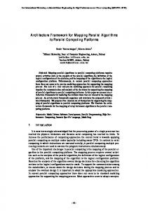
Fig. 2.1. Equivalence among structurally orthogonal column partition of A , distance-2 coloring of G(A) and distance-1 coloring of G 2 (A) . Top: symmetric case. Bottom: nonsymmetric case.

(by solving a rectangular system of equations). In this paper we focus on only direct methods. 2.2.1. Structurally orthogonal partition. Curtis, Powell, and Reid [9] showed that a structurally orthogonal partition of a Jacobian matrix A —a partition of the columns of A in which no two columns in a group share a nonzero at the same row index—gives a seed matrix S where the entries of A can be directly recovered from the compressed representation B ≡ AS . The structure of a Jacobian matrix A can be represented by the bipartite graph Gb (A) = (V1 , V2 , E) , where V1 is the row vertex set, V2 is the column vertex set, and (ri , cj ) ∈ E whenever the matrix entry aij is nonzero. A partitioning of the columns of the matrix A into groups consisting of structurally orthogonal columns is equivalent to a partial distance-2 coloring of the bipartite graph Gb (A) on the vertex set V2 [11]. It is called “partial” because the row vertex set V1 is left uncolored. A structurally orthogonal column partition could also be used in computing a Hessian via a direct method, albeit that symmetry is not exploited. Specifically, McCormick [20] showed that a structurally orthogonal partition of a Hessian is equivalent to a distance-2 coloring of its adjacency graph. The adjacency graph Ga (A) of a Hessian A has a vertex for each column, and an edge joins column vertices ci and cj whenever the entry aij , i 6= j , is nonzero; the diagonal entries in A are assumed to be nonzero and they are not explicitly represented by edges in the graph Ga (A) . Figure 2.1 illustrates how a structurally orthogonal column partition of a matrix is modeled by a distance-2 coloring in the appropriate graph. The right most subfigures show the equivalent distance-1 coloring formulations in the appropriate square graph. 2.2.2. Symmetry-exploiting partition. Powell and Toint [22] were the first to introduce a symmetry-exploiting technique for computing a Hessian via a direct method. When translated to a coloring φ of the adjacency graph, the partition Powell and Toint suggested for a direct Hessian computation requires that (1) φ be a distance-1 coloring, and (2) in every path v, w, x on three vertices, the terminal vertices v and x are allowed to have the same color, but only if the color of the


5

middle vertex w is lower in value. A coloring that satisfies these two requirements has been called a restricted star coloring in [14]. Coleman and Mor´e [8] showed that a symmetrically orthogonal partition of a Hessian is sufficient for a direct recovery, and established that such a partition is equivalent to a star coloring of the adjacency graph of the Hessian. A star coloring is a distance-1 coloring where, in addition, every path on four vertices uses at least three colors. The name is due to the fact that in a star-colored graph, a subgraph induced by any two color classes is a collection of stars. Note that the three coloring models for direct Hessian computation discussed here can be ranked in an increasing order of restriction (decreasing order of accuracy) as star coloring, restricted star coloring, distance-2 coloring. 2.3. Greedy coloring algorithms. An optimization problem associated with distance-k, restricted star, or star coloring asks for an appropriate coloring with the fewest colors, and each is known to be NP-hard [8, 14, 20]. In practice, greedy algorithms have been found effective in delivering good suboptimal solutions for these problems fast [7, 14]. A greedy algorithm for each of these problems progressively extends a partial coloring of a graph by processing one vertex at a time, in some order; there exist a number of effective ordering techniques that are based on some variation of vertex degree [7, 14]. In the step where a vertex v is colored, first, a set F of forbidden colors for the vertex v is obtained by exploring the appropriate neighborhood of v . Then, the smallest allowable color (not included in F ) is chosen and assigned to v . In the case of distance-1 coloring, such a greedy algorithm uses at most ∆ + 1 colors, where ∆ is the maximum degree-1 in the graph. The quantity ∆ + 1 is a lower bound on the optimal number of colors needed in a distance-2 coloring. Furthermore, the number of colors used by a greedy distance-2 coloring algorithm is bounded from above by min{∆2 +1, n} , where n is the number of vertices in the input graph. Using this bound, McCormick [20] showed that the greedy distance-2 coloring algorithm is √ an O( n) -approximation algorithm. Greedy algorithms for distance-1 and distance-2 coloring can be implemented such that their respective complexities are O(nd1 ) and O(nd2 ) . Gebremedhin et al. [14] have developed O(nd2 ) -time greedy algorithms for star and restricted star coloring. Their algorithm for star coloring takes advantage of the structure of the two-colored induced subgraphs—the collection of stars—and uses fairly complex data structures to maintain them. In this paper we develop parallel versions of the greedy algorithms for distance-2 and restricted star coloring. We considered the simpler variant, restricted star coloring, instead of star coloring, since restricted star coloring can be derived via a simple modification of the parallel algorithm for the distance-2 coloring problem, which is the main focus of this paper. 3. Design issues. The parallel distance-2 coloring algorithm proposed in this paper will be presented in detail in §4. Here we discuss the major issues that arise in the design of the algorithm and the assumptions and decisions we made around them. 3.1. Data distribution. The way in which the input graph is partitioned and mapped to processors has implications for both load balance and inter-processor communication. A graph could be partitioned among processors either by partitioning the vertex set or by partitioning the edge set. Traditionally, vertex partitioning has been the most commonly used strategy for mapping graphs (or matrices) to processors [3, 6, 10]. When a vertex partitioning is used, edges are implicitly mapped to

6


processors, with every crossing edge essentially being duplicated on the two processors to which its endpoints are mapped. For matrices, this corresponds to mapping of entire columns or rows to processors. To make our algorithm and its implementation more readily usable in other parallel codes, we assume that a vertex partitioning is used in distributing the graph among processors. A vertex partitioning classifies the vertices of the graph into two categories: interior and boundary. An interior vertex is a vertex all of whose distance-1 neighbors are mapped onto the same processor as itself. A boundary vertex has at least one distance-1 neighbor mapped onto a different processor. 3.2. Data duplication and communication mechanism. The next design issue is data duplication and its impact on information exchange. As stated earlier, when a vertex partitioning is used, every crossing edge is duplicated, and that was the approach used in our earlier work on distance-1 coloring [5]. In such a mapping strategy, it makes sense for each processor to store the colors of the off-processor endpoints of its crossing edges as this would require storing at most one extra color per crossing edge. In terms of communication, such a storage scheme necessitates each processor to send the colors of its boundary vertices to neighboring processors as soon as the colors become available. Each receiving processor could then store the information and use it later while coloring its own vertices. In this way, the color of a boundary vertex is sent at most once for each of its incident crossing edges. In the distance-2 coloring case, for each vertex, color information about vertices that are two edges away is also needed. One way of acquiring this information would be for each processor to keep a local copy of the subgraph induced by off-processor vertices that are within distance two edges from its own boundary vertices. Then, each processor could store and have access to all the needed color information as soon as the information is received from neighboring processors. Thus, as in the distance-1 coloring case, color information could be sent as soon as it becomes available. This would in turn allow for a flexible coloring order on each processor, since the order in which vertices are colored can be freely determined as the algorithm proceeds. However, this flexibility comes at the expense of extra storage. For relatively dense graphs, large portions of the input graph may need to be duplicated on each processor. In fact, this could happen even if there was just one high degree boundary vertex. For this reason, we chose to duplicate just the boundary vertices and their colors, but not more. With this design decision in place, each processor will gain local access to distance1 color information just like in the distance-1 coloring algorithm, and the information can be exchanged among the processors at the earliest possible time. But a mechanism for exchanging color information among vertices that are two edges apart still needs to be devised. Since such colors are not going to be stored permanently on the receiving processor, each color will have to be resent every time it is needed. Here, there are two basic ways in which the communication can be coordinated: one can use either a request-based protocol or a precomputed schedule. In a request-based protocol, each processor would send a message to its neighboring processors asking for specific color information whenever it needs the information. It then receives the information, uses it, and discards it. With a precomputed schedule, each processor would know the order (at least partially) in which its neighbor processors are going to color their vertices. Thus a processor could itself determine what color information to send to its neighbors and when to do so. A request-based protocol gives rise to more communication than a precomputed schedule, but on the other hand, it is more flexible as it allows for a


7

Algorithm 1 Overview of the parallel distance-2 coloring algorithm. 1: procedure ParallelColoring( G = (V, E), s ) 2: Data distribution: G is divided into p subgraphs G1 = (V1 , E1 ), . . . , Gp = (Vp , Ep ) ,

3: 4: 5: 6: 7: 8: 9: 10: 11:

where V1 , . . . , Vp is a partition of the set V and Ei = {(v, w) : v ∈ Vi , (v, w) ∈ E} . Processor Pi owns the vertex set Vi , and stores the edge set Ei and the ID’s of the processors owning the other endpoints of Ei . on each processor Pi , i ∈ P = {1, . . . , p} Ii ← interior vertices in Vi Bi ← boundary vertices in Vi . Vi = Ii ∪ Bi Color the vertices in Ii Assign each vertex v ∈ Bi ∪ N1 (Bi ) a random number rand(v) , generated using v ’s ID as seed Ui ← Bi . Ui is the current set of boundary vertices to be colored by Pi while ∃j ∈ P, Uj 6= ∅ do TentativelyColor( Ui ) Ui ← DetectConflicts()

completely independent coloring order on each processor. In our algorithm we chose to use a precomputed schedule. Even with a precomputed schedule, there exists an opportunity for using ordering techniques at a local level on each processor, but we fore-go a detailed study of such ordering techniques to limit the scope of this paper. 4. Parallel Distance-2 Coloring of General Graphs. We are now ready to present the new parallel distance-2 coloring algorithm for a general graph G = (V, E) . We begin in §4.1 by providing an overview of the algorithm, and then present its details layer-by-layer in §4.2 through §4.4. The complexity of the algorithm is analyzed in §4.5, and a brief discussion of possible variations of the algorithm is given in §4.6. In §5 we will show how the algorithm needs to be modified to solve the restricted star coloring problem on a general graph G and the partial distance-2 coloring problem on a bipartite graph Gb = (V1 , V2 , E) . 4.1. Overview of the algorithm. Initially, the input graph G = (V, E) is assumed to be vertex-partitioned and distributed among the p available processors. The set Vi of vertices in the partition { V1 , . . . , Vp } of V is assigned to and colored by processor Pi . We say Pi owns Vi . In addition, processor Pi stores the adjacency list of its vertices and the identities of the processors owning them. This initial data distribution classifies each set Vi into sets of interior and boundary vertices (Vi = Ii ∪ Bi ). We call two processors Pi and Pj neighbors if at least one boundary vertex owned by processor Pi has a distance-1 neighbor vertex owned by processor Pj . Clearly, any two interior vertices owned by two different processors can safely be colored concurrently in a distance-2 coloring. In contrast, a concurrent coloring of a pair of boundary vertices or a pair consisting of one boundary and one interior vertex may not be safe, as the constituents of the pair, while being distance-2 neighbors, may receive the same color and therefore result in a conflict. We avoid the latter situation for a potential conflict (due to a pair consisting of one boundary and one interior vertex) by requiring that interior vertices be colored strictly before or strictly after boundary vertices have been colored. Then, a conflict can occur only for pairs of boundary vertices. Thus, the central part of the algorithm being presented is concerned with how the coloring of the boundary vertices is performed in parallel. The main idea is to perform the coloring of the boundary vertices concurrently in

8


a speculative manner and then detect and rectify conflicts that may have arisen. The algorithm (iteratively) proceeds in rounds, each consisting of a tentative coloring and a conflict detection phase. Both of these phases are performed in parallel. To reduce the frequency of communication among processors, the tentative coloring phase is organized in a sequence of supersteps, a term borrowed from the literature on the Bulk Synchronous Parallel model [3] and used here in a loose sense. Specifically, in each superstep, each processor colors a pre-specified number s of the vertices it owns in a sequential manner, using forbidden color information available at the beginning of the superstep, and only thereafter sends recent color information to neighboring processors. In this scenario, if two boundary vertices that are either adjacent or at a distance of exactly two edges from each other are colored during the same superstep, they may receive the same color and thus cause a conflict. The purpose of the subsequent detection phase is to discover such conflicts in the current round and accumulate a list of vertices on each processor that needs to be recolored in the next round to resolve the conflicts. Given a pair of vertices involved in a conflict, it suffices to re-color only one of them to resolve the conflict. The vertex to be recolored is determined by making use of a global random function defined over all boundary vertices. In particular, each processor Pi assigns a random number to each vertex in the set Bi ∪ N1 (Bi ) , where Bi is the set of boundary vertices owned by Pi and N1 (Bi ) = ∪w∈Bi N1 (w) . Each random number rand(v) is generated using the global ID of the vertex v , to avoid the need for processors to inquire each other of random values. The algorithm terminates when no more vertices to be re-colored are left. A high-level structure of the algorithm is given in Algorithm 1. The routines TentativelyColor and DetectConflicts called in Algorithm 1 will be discussed in detail in §4.3 and §4.4, respectively. But first we discuss a few fundamental techniques employed in Algorithm 1. 4.2. Conflict detection and relaying distance-2 color information. In addition to the design issues on data distribution, data duplication, and communication protocol discussed in §3, the way in which conflicts are detected is a major issue in the design of Algorithm 1. We employed a strategy in which for every path v, w, x on three vertices, the processor on which the vertex w resides is responsible for detecting not only conflicts that involve the vertex w and an adjacent vertex in N1 (w) but also a conflict involving the vertices v and x. We call the former (involving adjacent vertices) type 1 conflicts, and the latter (involving vertices two edges apart) type 2 conflicts. A type 1 conflict is detected by both of the implied processors, whereas a type 2 conflict is detected by the processor owning the middle vertex. Clearly, this way of detecting a type 2 conflict is more efficient than the alternative in which the conflict is detected by both of the processors owning the terminal vertices v and x. As the termination condition of the while-loop in Algorithm 1 indicates, even if a processor has no more vertices left to be re-colored in a round, i.e., Ui = ∅ , it could still be active in that round, as the processor may need to provide color information to other processors, participate in detecting conflicts on other processors, or both. Another basic ingredient in the design of Algorithm 1 is the technique used to build the list of forbidden colors for a given vertex v in a given superstep. The technique is directly related with the strategies on data duplication and communication protocol employed in the design of the algorithm (these were discussed in §3.2). The next two paragraphs discuss elements of this technique. Let Pi be the processor that owns the vertex v . The list of forbidden colors for the vertex v consists of (1) colors assigned to adjacent vertices—those in the set

9


Pk Pi w2

x1 w1 x2

Pi

Pj w

v

x3

x

Pi

v

v

w

x1

(i)

(ii)

Pj x2

(iii)

Fig. 4.1. Scenarios depicting the distribution of the distance-2 neighbors of vertex v across processors.

N1 (v) —and (2) colors assigned to vertices exactly two edges away from v . These colors are assigned either in a previous superstep (for boundary vertices) or prior to the iterative coloring (for interior vertices). We classify these colors as local or nonlocal relative to processor Pi on the onset of the superstep. A color of a vertex u is local to Pi if Pi owns either the vertex u or some distance-1 neighbor of u (in which case Pi would store a copy of u ’s color information, which is computed and sent by u ’s owner). In contrast, a color is nonlocal to Pi if the information is not locally stored and hence needs to be relayed via an “intermediate” processor. Figure 4.1 shows the three scenarios in which the vertices on a path v, w, x may be distributed among processors. Case (i) corresponds to the situation where both of the vertices w and x (w1 and x1 or w2 and x2 in the figure) are owned by processor Pi . Clearly, in this case, the colors of the vertices w and x are both local to Pi . Case (ii) shows the situation where vertex w is owned by processor Pi and vertex x is owned by processor Pj , j 6= i. In this case, again, the colors of both vertices w and x are local to Pi . Case (iii) shows the situation where vertex w is owned by processor Pj , and vertices v and x do not have a common distance-1 neighbor owned by processor Pi . As depicted in the figure, vertex x may be owned by any one of the three processors Pi , Pj , or Pk , i 6= j 6= k (shown as vertices x1 , x2 , and x3 , respectively). In this third case, if the vertex x is owned by either of the processors Pj or Pk (shown as x2 and x3 ), then the color of x is nonlocal to processor Pi and needs to be relayed to Pi through processor Pj . On the other hand, if the vertex x is owned by processor Pi (shown as x1 ), then the color of x is, strictly speaking, local to Pi and need not be relayed via Pj . However, in the algorithm being described, since processor Pj does not store the adjacency lists of the vertices owned by processor Pi , it would treat the color of x1 as if it were nonlocal to Pi and send the color information to Pi . In other words, for every edge (v, w) in which vertex v is owned by processor Pi and w is owned by Pj , processor Pj takes the responsibility of building a list of colors used by vertices two edges away from the vertex v (a partial list of forbidden colors to v ) and sending the list to processor Pi . 4.3. The tentative coloring phase. Algorithm 2 outlines in detail the routine TentativelyColor run on each processor Pi . The routine starts off by processor Pi determining a coloring-schedule—a breakdown of its current set Ui of vertices to be colored into supersteps (Line 2). Processor Pi then computes and sends schedule information to each of its neighboring processors (Lines 3–5). Similarly, processor Pi receives analogous schedules from each of its neighboring processors (Line 6). This enables each processor to know the distance-2 color information it needs to send in

10


Algorithm 2 Tentative coloring phase of Algorithm 1 run on processor Pi . 1: procedure TentativelyColor( Ui ) 2: Partition Ui into ni subsets Ui,1 , Ui,2 , . . . , Ui,ni , each of size s . ni = d |Usi | e . Vertices in Ui,` will be colored in the ` ’th superstep by processor Pi 3: for each processor-superstep pair (j, l) ∈ {{1, . . . , p} × {1, . . . , ni }} , j 6= i do j 4: Ui,` ← {v|v ∈ Ui,` and N1 (v) ∩ Vj 6= ∅} . processor Pj is neighbor to processor Pi 5: 6: 7: 8: 9: 10: 11: 12: 13: 14: 15: 16: 17: 18: 19: 20: 21:

j to each neighbor processor Pj Send schedules Ui,` i Receive S schedules Uj,` from each neighbor processor Pj i Xi,` ← j Uj,` . Vertices in Xi,` will be colored in the ` ’th step by processors Pj , j 6= i S for each v ∈ Xi ∪ Ui , where Xi = ` Xi,` do color(v) ← 0 . (re)initialize colors L ← max1≤j≤p {nj } . L is the max number of supersteps over all processors for ` ← 1 to L do . each ` corresponds to a superstep i Build lists of forbidden colors for vertices in Uj,` Send the lists to each neighboring processor Pj where ` ≤ nj if ` ≤ ni then . Pi has not finished coloring Ui j Receive lists of forbidden colors for vertices in Ui,` from each neighboring Pj Merge the lists of forbidden colors Update the lists of forbidden colors with local color information for each v ∈ Ui,` do color(v) ← c such that c > 0 is the smallest “permissible” color for v j Send updated colors of vertices in Ui,` to each neighboring Pj i Receive updated colors of vertices in Uj,` from each neighboring Pj

each superstep. In particular, using the schedules, for each superstep `, processor Pi constructs a list Xi,` of vertices that will be colored by some other processor Pj in superstep ` and for which it must supply forbidden color information (Line 7). Thus with the knowledge of each Xi,` , processor Pi can be “pro-active” in building up lists of relevant forbidden color information and sending these to neighboring processors in superstep `. Before the coloring of the vertices in the set Ui by processor Pi commences, impermissible colors assigned in a previous superstep need to be cleared. These consist of colors assigned to vertices in Ui (by processor Pi ) and colors assigned to vertices in Xi , which are to be colored by other processors in the current round (Lines 8 and 9). Since for different processors Pi the number of vertices |Ui | to be colored could differ, the number of supersteps required to color these vertices, ni = d |Usi | e , would also vary. Processor Pi needs ni supersteps to color its vertices, but it may need to supply forbidden color information to a neighboring processor that has not finished coloring its vertices. Therefore, the algorithm overall needs L = max1≤j≤p {nj } supersteps (see Line 10). In each superstep, before processor Pi begins to color the set of vertices it owns, it pro-actively builds and sends relevant color information to neighboring processors (Lines 12 and 13). Further, to perform the coloring of its own vertices in a superstep, a processor first gathers color information from other processors to build a partial list of forbidden colors for each of its boundary vertices scheduled to be colored in the current superstep. After the processor has received the partial lists of forbidden colors from all of its neighboring processors, it merges these lists and augments them with local color information to determine a complete list of forbidden colors for its vertices scheduled to be colored in the current superstep. Using this information, the


11

Algorithm 3 Conflict detection phase of Algorithm 1 run on processor Pi . 1: function DetectConflicts 2: Wi ← ∅ . Wi is the set of vertices Pi examines to detect conflicts 3: for ` ← 1 to L do . uses schedules computed in Algorithm 2 4: for each w ∈ Ui,` where w has at least one neighbor in Xi,` do 5: Wi ← Wi ∪ {w} . w is used for detecting type 1 conflicts 6: for each w ∈ Vi where w has at least two neighbors in Xi,` ∪ Ui,` on different 7: 8: 9: 10: 11: 12: 13: 14: 15: 16: 17: 18: 19: 20: 21: 22: 23: 24: 25: 26: 27: 28: 29: 30:

processors do Wi ← Wi ∪ {w} . w is used for detecting type 2 conflicts for each j ∈ P = {1, . . . , p} do Ri,j ← ∅ . Ri,j is a set of vertices Pi notifies Pj to recolor for each w ∈ Wi do encountered[color(w)] ← w lowest[color(w)] ← w for each x ∈ N1 (w) do if encountered[color(x)] = w then v ← lowest[color(x)] if rand(v) ≤ rand(x) then . rand(u) : random number assigned to u if v 6= w then Ri,Id(x) ← Ri,Id(x) ∪ {x} . Id(u) : ID of processor owning u else Ri,Id(v) ← Ri,Id(v) ∪ {v} lowest[color(x)] ← x else encountered[color(x)] ← w lowest[color(x)] ← x for each j ∈ P , j 6= i do Send Ri,j to processor Pj for each j ∈ P , j 6= i do Receive Rj,i from processor Pj Ri,i ← Ri,i ∪ Rj,i return Ri,i

processor then speculatively colors the vertices of the current superstep. At the end of the superstep, the new color information is sent to neighboring processors. These actions are performed in the piece of code in Lines 14–20. Regardless of whether a processor has finished coloring all of its vertices or not, it needs to receive updated color information from neighboring processors (see Line 21). This information is needed to enable the processor to compile forbidden color information to be sent to other processors in the next superstep. 4.4. The conflict detection phase. Algorithm 3 outlines the conflict detection routine DetectConflicts executed on each processor Pi . The routine has two major parts. In the first part, the routine finds a subset Wi ⊂ Vi of vertices processor Pi needs to examine to detect both type 1 and type 2 conflicts. Whenever a conflict is detected, one of the involved vertices is selected to be recolored in the next round to resolve the conflict. The selection makes use of the random values assigned to boundary vertices in Algorithm 1. In the second part, the routine determines and returns a set of vertices to be recolored by processor Pi in the next round. Two vertices would be involved in a conflict only if they are colored in the same superstep. Thus the vertex set Wi need only consist of (1) every vertex v ∈ Ui that has at least one distance-1 neighbor on a processor Pj , j 6= i, colored in the

12


same superstep as v , and (2) every vertex v ∈ Vi that has at least two distance-1 neighbors on different processors that are colored in the same superstep, since these might be assigned the same color. To obtain elements of the set Wi that satisfy one or both of these two conditions in an efficient manner, in Algorithm 3, relevant vertices on processor Pi are traversed a superstep at a time, using the schedule computed in Algorithm 2. In each superstep `, first each vertex in Ui,` and its neighboring boundary vertices are marked. Then, for each vertex v ∈ Xi,` the vertices in the set N1 (v) owned by processor Pi are marked. If this causes some vertex to be marked twice during the same superstep, then the vertex is added to Wi . The determination of the set Wi is achieved by the piece of code in Lines 3–7 of Algorithm 3; details are omitted for brevity. Turning to the second part of Algorithm 3, processor Pi accumulates a list Ri,j of vertices to be recolored by each processor Pj in the next round. To detect conflicts around a vertex w in the set Wi , we need to look for vertices in the set N1 (w) ∪ {w} that have the same color. In a valid distance-2 coloring, every vertex in the set N1 (w)∪ {w} needs to have a distinct color. If several vertices with the same color are found, we let the vertex with the lowest random value keep its color and re-color the rest. To perform these tasks efficiently, we use two color-indexed, one-dimensional, arrays— encountered and lowest —that store vertices. The values stored in the two arrays encode information that is updated and used in a for-loop that iterates over each vertex w ∈ Wi . The context in each iteration in turn is a visit through the neighborhood N1 (w) of the vertex w . For each vertex w , encountered[c] = w indicates that at least one vertex in N1 (w) ∪ {w} having the color c has been encountered, and lowest[c] stores the vertex with the lowest random value among these. Initially, both encountered[color(w)] and lowest[color(w)] are set to be w . This ensures that any conflict involving the vertex w and one of the vertices in the set N1 (w) would be discovered. To detect conflicts involving the neighbors of w , the algorithm checks whether a given color used by a vertex in N1 (w) has been encountered more than once, and if so, the vertex to be recolored is determined using the random values assigned to the vertices and the array lowest is updated accordingly. See the for-loop in Lines 10–24 for details. In Algorithm 3, a type 1 conflict involving adjacent vertices is detected by both of the implied processors. Thus the if-test in Line 17 is included to avoid sending unnecessary notification from one processor to the other. Note also that in Line 13, it would have been sufficient to check for conflicts only using vertices N1 0 (w) ⊆ N1 (w) that belong to either Ui or Xi . However, since determining the subset N1 0 (w) takes more time than testing for a conflict, we use the larger set N1 (w) in Line 13. When the lists Ri,j processor Pi accumulates are complete, processor Pi sends each list Ri,j to processor Pj , j 6= i, to notify the latter to do the re-coloring (Lines 25–26). Processor Pi itself is responsible for re-coloring the vertices in Ri,i and therefore adds to Ri,i notifications Rj,i received from each neighboring processor Pj (Lines 27–29). 4.5. Complexity. In Algorithm 2, the overall sequential work carried out by processor Pi and its neighboring processors in order to perform the coloring of the vertices in Ui is O(Σv∈Ui d2 (v)) . Summing over all processors, the total work (excluding communication cost) involved in coloring the vertices in the set U = ∪Ui is O(Σv∈U d2 (v)) , which is equivalent to the complexity of a sequential algorithm for coloring the vertex set U . Turning to the communication cost involved in Algorithm 2, note that for each


13

vertex v ∈ Ui , every neighboring processor sends to processor Pi the union of the colors used by vertices at exactly two edges from the vertex v , while the color of the vertex v is sent to every processor that owns a distance-1 neighbor of v . Thus the total size of data exchanged while coloring the vertex v is bounded by O(d2 (v)) , which in turn gives the bound O(Σv∈U d2 (v)) , where U = ∪Ui , on the overall communication cost of Algorithm 2. In Algorithm 3, in determining the set Wi (in Lines 3–7), at most |Vi | vertices are processed. The per-vertex work involved in this process is proportional to the degree1 of the vertex. Hence, the time needed to determine Wi is bounded by O(|Vi |d1 ) , where d1 is the average degree-1 in the input graph G . Further, in each iteration of the for-loop over the set Wi in Lines 10–24, the set of vertices to be recolored is determined in time O(d1 (w)) , which gives a complexity of O(|Wi |d1 ) for the entire for-loop. Since |Wi | ≤ |Vi | clearly holds, the overall complexity of Algorithm 3 is O(|Vi |d1 ) . With the complexities of Algorithms 2 and 3 just established and assuming that the number of rounds required in Algorithm 1 is sufficiently small, the total work carried out by all of the p processors in coloring the input graph G = (V, E) is O(|V|d2 ) , which is the same as the complexity of the sequential algorithm. The experimental results reported in §6 attest that the number of rounds for large-size graphs that arise in practice is indeed fairly small; the observed number was about half a dozen in most cases, and never more than a few dozens, while coloring graphs with millions of edges and employing as many as a hundred processors. 4.6. Variations. Algorithm 1 and its subroutines Algorithms 2 and 3 could be specialized along several axes to result in a variety of derived algorithms. We discuss three of these axes. First, in Algorithm 1, interior vertices ( Ii ) are colored before boundary vertices (Bi ), but the reverse order could also be considered. Second, while coloring the vertices in a superstep on each processor (see Line 18 of Algorithm 2), the natural ordering of the vertices, a random ordering, or any other degree-based ordering technique could be used [14]. Third, the choice of a color for a vertex in a superstep (see Line 19 of Algorithm 2) could be done in several different ways. For example, a First Fit (FF), a Staggered First Fit (SFF), or a randomized coloring strategy could be used [5]. In the FF strategy, each processor chooses the smallest allowable color for a vertex, starting from color 1. In the SFF strategy, each processor Pi chooses the smallest permissible color from the set {d iK p e, . . . , K} , where the initial estimate K is set to be, for example, equal to the lower-bound ∆ + 1 on the distance-2 chromatic number. If no such color exists, then the smallest permissible color in {1, . . . , b iK p c} is chosen. If there still is no such color, the smallest permissible color greater than K is chosen. Since the search for a color in SFF starts from different “base colors” for each processor, SFF is likely to result in fewer conflicts than FF. 5. Parallel Restricted Star and Partial Distance-2 Coloring. The algorithms presented in the previous section need to be modified only slightly to solve the two related problems of our concern, restricted star coloring on a general graph (for Hessian computation) and partial distance-2 coloring on a bipartite graph (for Jacobian computation). In this section we point out the specific changes that need to be made in Algorithms 1–3 to address these two problems.

14


Algorithm 4 Basic difference between distance-2 and partial distance-2 coloring. procedure D2Coloring( G = (V, E) ) for each v ∈ V do for each w ∈ N1 (v) do Forbid color(w) to v for each x ∈ N1 (w) do Forbid color(x) to v Assign a color to vertex v

procedure PD2Coloring( Gb = (V1 , V2 , E) ) for each v ∈ V2 do for each w ∈ N1 (v) do . w ∈ V1 never receives a color for each x ∈ N1 (w) do Forbid color(x) to v . x ∈ V2 Assign a color to vertex v

5.1. Restricted star coloring. As the definition given in §2.2 implies, in a restricted star coloring of a graph, the color assigned to a vertex v needs to satisfy conditions that concern the distance-2 neighbors N2 (v) of the vertex v . The exact same neighborhood is consulted in assigning a color for the vertex v in a distance2 coloring of the graph. Therefore, the greedy algorithms for the two variants of coloring (as developed in [14]) differ only in the way the set of forbidden colors for the vertex v is determined. We describe this difference below in the sequential setting; the additional differences that arise in the parallel setting are fairly straightforward to implement and their discussion is omitted. Consider the step of a greedy algorithm (distance-2 or restricted star coloring) in which the vertex v is to be colored, and let v, w, x be a path in the distance-2 neighborhood of the vertex v . In the distance-2 coloring algorithm, both color(w) and color(x) are forbidden to the vertex v , since the path needs to have three distinct colors. In the restricted star coloring algorithm, on the other hand, color(w) would always be forbidden to v , whereas color(x) may or may not be forbidden. The decision in the latter case is made based on further tests: • If color(w) = 0 (i.e., vertex w is not yet colored), then color(x) is forbidden to v . This ensures that any extension v, w, x, y of the path v, w, x would end up using at least three colors, as desired, since in the step in which the vertex w is colored, the distance-1 coloring requirement guarantees that the vertex w gets a color distinct from color(v) and color(x) . • If color(w) 6= 0 , then color(x) is forbidden to v only if color(w) > color(x) . 5.2. Partial distance-2 coloring. Here, the input is a bipartite graph Gb = (V1 , V2 , E) , and only the vertex set V2 needs to be colored satisfying the condition that a pair of vertices from V2 sharing a common distance-1 neighbor in V1 receive different colors. If not already distributed, the graph Gb needs to be partitioned among the processors in a manner that minimizes boundary vertices (and hence the likelihood of conflicts and the size of overall communication). Assuming a vertex partitioning is used, let V1,1 , . . . , V1,p denote the partitioning of the set V1 , and let V2,1 , . . . , V2,p denote the partitioning of the set V2 . The subgraph assigned to processor Pi would then be Gb,i = (V1,i , V2,i , Ei ) , where Ei is the set of edges incident on vertices in V1,i ∪V2,i . In terms of the underlying matrix, such a partitioning means that each processor owns a subset of the rows as well as a subset of the columns; this is in contrast with the case where either only the columns or only the rows are partitioned. With such a partitioning in place, the only change that needs to be made in Algorithm 1 is to replace the two references to Vi (in Lines 4 and 5) with V2,i . The changes that need to be made in Algorithms 2 and 3 are minimal as well, and they are consequences of the basic difference between distance-2 coloring in a general graph G = (V, E) and partial distance-2 coloring in a bipartite graph Gb = (V1 , V2 , E) illustrated by the code fragment in Algorithm 4.


15

Table 6.1 Structural properties of the application (top), and the synthetic (bottom) test graphs used in the experiments. The last column shows the number of edges in G 2 = (V, F ) compared to G = (V, E) . (ST–Structural Engineering [26], SH–Ship Section [28], CA–Linear Car Analysis [28], AU– Automotive [26], CE–Civil Engineering [26]). app/ class ST

SH

CA

AU

CE planar random random s. world s. world

name

|V|

|E|

nasasrb ct20stif pwtk shipsec8 shipsec1 shipsec5 bmw7st1 bmw3 2 inline1 hood msdoor ldoor pkustk10 pkustk11 pkustk13 plan-1 rand-1 rand-2 sw-1 sw-2

54,870 52,329 217,918 114,919 140,874 179,860 141,347 227,362 503,712 220,542 415,863 952,203 80,676 87,804 94,893 4,072,937 400,000 400,000 400,000 400,000

1,311,227 1,323,067 5,708,253 3,269,240 3,836,265 4,966,618 3,599,160 5,530,634 18,156,315 5,273,947 9,912,536 22,785,136 2,114,154 2,565,054 3,260,967 12,218,805 2,002,202 4,004,480 1,998,542 3,993,994

Degree max avg 275 48 206 51 179 52 131 57 101 55 125 55 434 51 335 49 842 72 76 48 76 48 76 48 89 52 131 58 299 69 40 6 27 10 45 20 468 10 880 20

colors d1 d2 41 276 49 210 48 180 54 150 48 126 50 140 54 435 48 336 51 843 42 103 42 105 42 112 42 126 66 198 57 303 9 41 9 41 12 101 18 469 27 882

exec. time (s) d1 d2 0.049 2.237 0.063 2.581 0.229 10.335 0.128 6.776 0.143 7.457 0.190 9.852 0.167 6.730 0.274 10.077 0.925 55.217 0.277 9.407 0.520 17.438 1.197 40.180 0.091 3.904 0.103 6.041 0.155 9.302 3.435 18.880 0.644 6.676 1.242 21.977 0.345 13.909 0.632 50.954

|F | |E|

3.2 3.8 2.9 3.5 3.1 3.2 3.3 3.2 7.0 3.2 3.2 3.2 2.9 4.2 6.0 3.4 11 21 31 59

6. Experiments. In this section we present results on experimental evaluation of the performance of the algorithms presented in the previous two sections. The algorithms are implemented in C using the MPI message-passing library. 6.1. Experimental setup. Test platform. The experiments are carried out on a 96-node PC cluster equipped with dual 2.4 GHz Intel P4 Xeon CPUs and 4 GB memory. The nodes of the cluster are interconnected via a switched 10Gbps Infiniband network. Test graphs. Our first test set consists of 15 real-world graphs obtained from five different application areas: structural engineering, ship section design, linear car analysis, automotive design, and civil engineering [12, 24, 26, 28]. The top part of Table 6.1 lists the number of vertices, number of edges, maximum degree-1, and average degree-1 in each of these test graphs. The graphs are classified according to the application area they are drawn from. Table 6.1 also lists the number of colors and the execution time in seconds used by greedy sequential distance-1 and distance2 coloring algorithms when each is run on a single node of our test platform. The last column lists the ratio between the number of edges in the square graph G 2 and the number of edges in G . These computed quantities will be used to gauge the performance of the proposed parallel coloring algorithms on the input graphs G . To be able to study the scalability of the proposed algorithms on a wider range of graph structures, we have also run experiments on synthetically generated graphs, which constitute our second test set. To represent extreme cases, the synthetic graphs considered included instances drawn from three different graph classes: random, planar and small-world graphs. (Loosely speaking, a small-world graph is a graph in which the distance between any pair of non-adjacent vertices is fairly small.) The

16


random and small-world graphs are generated using the GTgraph Synthetic Graph Generator Suite [27]. The planar graphs are maximally planar—the degree of every vertex is at least five—and are generated using the expansion method described in [21]; the generator is a part of the graph suite for the Second DIMACS Challenge [25]. The structural properties of these graphs as well as the number of colors and runtime used by sequential distance-1 and distance-2 coloring algorithms run on them are listed in the bottom part of Table 6.1. In the runtimes reported in Table 6.1 as well as in later figures in this section, each individual test is an average of five runs. In the timing of the parallel coloring code, we assume that the graph is initially partitioned and distributed among the nodes of the parallel machine, and thus the times reported concern only coloring. In all of the experiments, the input graph is partitioned using the tool MeTiS [17]. 6.2. Performance of the sequential algorithms. Before we proceed with evaluating the performance of the proposed parallel coloring algorithms, it is worthwhile to observe that the underlying sequential greedy algorithms, in both the distance1 and the distance-2 coloring cases, performed remarkably well in terms of number of colors used on both the application and synthetic test graphs. Specifically, as Table 6.1 shows, the number of colors used by the greedy sequential distance-1 coloring algorithm is in most cases slightly below the average degree and far below the maximum degree, which is an upper bound on the optimal solution (the distance-1 chromatic number). Even more remarkably, the number of colors used by the greedy sequential distance-2 coloring algorithm in most cases is observed to be very close to the maximum degree, which is a lower bound on the optimal solution (the distance-2 chromatic number). Thus the solution obtained by the greedy distance-2 coloring algorithm is in most cases either optimal or just a few colors more. In both of these greedy algorithms, the vertices were colored in the natural order they appear in the input graphs. 6.3. Results on parallel distance-2 coloring. In this section we present detailed experimental results on the parallel distance-2 coloring algorithm for general graphs discussed in §4. In §6.4 we shall present results on the related algorithms, restricted star coloring on general graphs and partial distance-2 coloring on bipartite graphs. In §6.6 we present results on the alternative approach of obtaining a distance-2 coloring by distance-1 coloring the square graph. 6.3.1. Choice of superstep size. Our first set of experiments, the results of which is given in Figure 6.1, is conducted to study the dependence of the performance of Algorithm 1 on the choice of the superstep size s, the number of vertices colored in a superstep before communication takes place. The experiments are conducted using the application test graphs and the reported results are averages over each class, while using 32 processors . We obtained similar results while experimenting with various other number of processors, but we report only for 32 processors for space considerations. Figure 6.1(a) shows a plot of the number of conflicts, normalized relative to the total number of vertices in the graph, as a function of superstep size. As one would expect, the normalized number of conflicts and the number of rounds (not shown here) increased as the superstep size s was increased, but the rate of increase remained fairly low once the value of s passed a few hundred. Figure 6.1(b) shows that, for values of s above a few hundred, further increase in s does not significantly influence speedup. Similarly, our experiments (not shown here) showed that the number of colors does

17

PARALLEL GRAPH COLORING FOR DERIVATIVE COMPUTATION 0.16

0.12

AU ST SH CA CE

25

20

0.1

Speedup

Number of conflicts / |v|

0.14

0.08 0.06

15

10

0.04

AU ST SH CA CE

5 0.02 0 0

500

1000

1500

2000

Superstep size

(a)

2500

3000

0 0

500

1000

1500

2000

2500

3000

Superstep size

(b)

Fig. 6.1. Normalized number of conflicts and speedup, while varying superstep size s for p = 32 .

not vary significantly with s, and stays within 12% of the number of colors used by the sequential algorithm. In general, an “optimal” value for s is likely to depend on both the properties of the graph being colored (size and density) and the platform on which the algorithm is executed. Based on observations from our parallel experiments, we used a superstep size of 100 for the scalability studies we report on in the rest of this section. 6.3.2. Strong scaling results. Our second set of experiments is concerned with the strong scalability of the parallel distance-2 coloring algorithm as the number of processors used is varied. This set of experiments was conducted on both the application and synthetic test graphs. The results from the experiments on the application graphs are summarized in Figure 6.2, and those from the synthetic graphs are summarized in Figure 6.3. In the results shown in Figure 6.2, the largest graph from each application category was used. A more detailed set of results on all of the application test graphs for the distance-2 as well as the restricted star coloring algorithm is included in a table in the Appendix. Results on application test graphs. The results in Figures 6.2(a) and 6.2(b) show that the number of conflicts and the number of rounds increase with increasing number of processors. However, the rate of growth as well as the actual values of both of these quantities was observed to be fairly small for all graphs except pkustk13 and inline1, the densest graphs in our test set. The reason for the relatively large number of rounds required in coloring the graph inline1 is the existence of vertices with very large degree-1. This phenomenon will be explained further with the help of synthetic graphs shortly. The metrics number of conflicts and number of rounds are in some sense “intermediate” performance measures for our parallel coloring algorithms. They are included in the reports to help explain results on the two ultimate performance metrics—speedup and number of colors used. The lower row of Figure 6.2 shows results on the latter two metrics. We will use a similar set of four metrics in several other experiments reported in this section. The speedup results in Figure 6.2(c) demonstrate that our algorithm in general scales well with increasing number of processors. As expected, the obtained speedup is relatively poorer in the cases where the number of conflicts and the number of rounds is relatively higher. The proposed algorithm also performed well in terms of the number of colors used. The results in Figure 6.2(d) show that the number of

18

˘ C ¨ ¨ ¨ BOZDAG, ¸ ATALYUREK, GEBREMEDHIN, MANNE, BOMAN, AND OZG UNER 20

0.09

ldoor pwtk shipsec5 inline_1 pkustk13

16

0.08 0.07 0.06 0.05 0.04 0.03 0.02

14 12 10 8 6 4

0.01 0 0


18

Number of rounds


0.1

2 20

40

60

80

0

100

20

40

(a)

Speedup

50


40

30

20

10

0 0

20

40

60

80

Number of processors

(c)

80

100

(b)

Normalized number of colors

60

60



100

1.15 1.1 1.05 1 0.95 0.9 0.85 0.8 0

ldoor pwtk shipsec5 inline_1 pkustk13 20

40

60

80

100


(d)

Fig. 6.2. Normalized number of conflicts (a), number of rounds (b), speedup (c), and normalized number of colors (d) while varying the number of processors for the application test graphs. In all cases, superstep size s = 100 was used.

colors used by our parallel algorithm, when as many as 96 processors are used, is at most 12% more than that used by the sequential algorithm. Recall that the solution obtained by the sequential algorithm in most cases is nearly optimal. Results on synthetic test graphs. We now turn attention to results on the synthetic graphs, which are designed to capture “extreme cases”. The planar graph plan-1 represents extremely well partition-able graphs—almost all of the vertices of plan-1 were interior vertices in a partition obtained using the tool MeTiS [17]. For such graphs parallel speedup in the context of Algorithm 1 comes largely from graph partitioning (data distribution) as opposed to the iterative coloring part. As Figure 6.3 shows this results in very small number of conflicts and good speedup. The random graphs rand-1 and rand-2 represent the opposite extreme—almost all of the vertices in these graphs are boundary regardless of how the graph is partitioned. As expected, Figure 6.3 shows that the number of conflicts is considerably larger for the random graphs. Nonetheless, our algorithm achieved some speedup (a constant around 10) even under such an extreme case. Note that the speedup in this case comes solely from the iterative coloring part. As mentioned earlier, graphs having vertices with very large degrees comprise a particularly difficult set of instances for the proposed parallel distance-2 coloring algorithm. Resolving conflicts involving the neighbors of such vertices requires a

19


1

160

plan−1 rand−1 rand−2 sw−1 sw−2

140

Number of rounds


1.2

0.8

0.6

0.4

120


100 80 60 40

0.2 20

0 0

20

40

60

80

100

0

20


40

60

80

100


(a)

(b)

90

70



80

Speedup

60 50 40 30 20 10 0 0

20

40

60

80


(c)

100

1.4

1.3

1.2

1.1

1

0.9

0.8 0

plan−1 rand−1 rand−2 sw−1 sw−2 20

40

60

80

100


(d)

Fig. 6.3. Normalized number of conflicts (a), number of rounds (b), speedup (c), and normalized number of colors (d) while varying the number of processors for the synthetic test graphs. In all cases, superstep size s = 100 was used.

large number of rounds which in turn degrades speedup. The third category in our synthetic graphs, the small-world graphs sw-1 and sw-2, are included to represent such a class of pathological instances for our approach. As Figure 6.3 shows, even though the number of conflicts for small-world graphs is not necessarily larger than that for random graphs with similar sizes, coloring small-world graphs required significantly larger number of rounds. Consequently, the speedup achieved was poorer—it was around 3 for all numbers of processors we experimented with. As can be seen from Figure 6.3(d), the normalized number of colors for all the synthetic graphs except rand-2 is within 12% of the sequential algorithm. For rand-2, there are relatively many conflicts but few rounds. This entails that many processors recolor a fairly large number of vertices in each round to resolve the conflicts. Over multiple rounds, this results in a significant increase in the number of colors used. This is in contrast to small world graphs, where many fewer vertices are recolored in many more rounds. This resembles sequential coloring, hence the number of colors increases only slightly. 6.3.3. Weak scaling. Our next set of experimental results is on weak scalability, where both problem size and number of processors are increased in proportion so as to result in nearly constant runtime. The experiments were conducted on five instances from each of random and planar graph classes. The structural properties of these

20

˘ C ¨ ¨ ¨ BOZDAG, ¸ ATALYUREK, GEBREMEDHIN, MANNE, BOMAN, AND OZG UNER 7

|V|

|E|

plan-2 plan-3 plan-4 plan-5 plan-6 rand-3 rand-4 rand-5 rand-6 rand-7

1,625,972 3,250,939 4,888,479 6,513,589 8,150,267 160,000 320,000 480,000 640,000 800,000

4,877,910 9,752,811 14,665,431 19,540,761 24,450,795 1,600,528 3,201,327 4,803,946 6,403,242 8,005,505

random planar

Degree max avg 37 6 43 6 43 6 38 6 39 6 45 20 46 20 43 20 44 20 45 20

6

Run time (seconds)

name

5

4

3

2

1

0 0

10

20

30

40

50

60

70

80

90


Fig. 6.4. Properties of the synthetic test graphs used in weak scaling tests (left) and results for distance-2 coloring (right).

1

160


140

Number of rounds


1.2

0.8

0.6

0.4

120


100 80 60 40

0.2 20

0 0

20

40

60

80

100

0

20


40

60

80

100


(a)

(b)

90

70



80

Speedup

60 50 40 30 20 10 0 0

20

40

60

80


(c)

100

1.4

1.3

1.2

1.1

1

0.9

0.8 0

plan−1 rand−1 rand−2 sw−1 sw−2 20

40

60

80

100


(d)

Fig. 6.5. Normalized number of conflicts (a), number of rounds (b), speedup (c), and normalized number of colors (d) while using SFF color selection strategy and varying the number of processors for the synthetic graphs in Table 6.1. Superstep size s = 100 .

graphs and the experimental results are summarized in Figure 6.4. It can be seen that the algorithm behaved almost ideally for planar graphs—the runtime remained nearly constant as the problem size and the number of processors were increased in proportion. For the random graphs, the runtime grew, but it did so fairly slowly.

21


Speedup

50



60

40

30

20

10

0 0

20

40

60

80


(a)

100

1.4

1.3


1.2

1.1

1

0.9

0.8 0

20

40

60

80

100


(b)

Fig. 6.6. Speedup (a) and normalized number of colors (b) for the restricted star coloring algorithm.

6.3.4. Variations of the algorithm. In the results presented thus far in this section, a variant of the proposed distance-2 coloring algorithm with the following combination of parameters was used: interior vertices were colored before boundary vertices; the natural ordering of the vertices was used while coloring; and a FF color choice strategy was employed. In addition to this “default” variant, we experimented with seven other variations in which interior vertices are colored after boundary vertices, a random vertex ordering is used while coloring, and a SFF color choice strategy (as discussed in §4.6) is used. The experiments showed that the only option that resulted in better performance in the majority of the test cases compared to the default variant was the use of the SFF coloring strategy. Figure 6.5 shows the performance of the SFF-coloring based variant on the synthetic test graphs. Results on the application graphs are omitted as no significant improvement over the FF-based variant was observed. As Figure 6.5 shows, the performance improvement with SFF was especially significant for the random and small-world graphs. The number of conflicts and the number of rounds were much smaller for these graphs when SFF is used instead of FF; hence better speedup was achieved. For small-world graphs, the SFF strategy required significantly more colors than FF, whereas for random graphs SFF required about the same number of colors for the random graph rand-1, and fewer colors for the denser random graph rand-2. 6.4. Results on parallel restricted star coloring. As discussed in §5, a parallel restricted star coloring of a graph can be obtained via a slight modification of the parallel distance-2 coloring algorithm. We have performed the necessary modifications and carried out experiments on the scalability of the resulting restricted star coloring algorithm. Figure 6.6(a) shows speedup results obtained when the restricted star coloring algorithm was run on the largest graph from each of the application graph classes listed in Table 6.1. As expected, these speedup results are very similar to those for distance-2 coloring (Figure 6.2(c)). The normalized number of colors used by the restricted star coloring algorithms are given in Figure 6.6(b). As results in the table in the appendix show, for many of the test graphs, restricted star coloring gives fewer colors than distance-2 coloring, demonstrating the advantage of exploiting symmetry.

22


Table 6.2 Structural properties of the additional test graphs [26] used for partial distance-2 coloring and experimental results. name

|V1 |

|V2 |

|E|

lhr71c stormG2 cont11 l cage13 cage14

70,304 528,185 1,468,599 445,315 1,505,785

70,304 1,377,306 1,961,394 445,315 1,505,785

1,528,092 3,459,881 5,382,999 7,479,343 27,130,349

sequential cols. time 65 1.43 48 0.85 8 0.52 118 2.27 136 8.86

speedup/num. of colors p=16 p=48 p=96 11.3/66 13.8/67 6.8/66 7.5/48 7.1/48 3.0/48 5.2/12 6.9/13 5.3/13 4.6/114 4.2/119 2.7/113 3.4/129 4.9/131 3.5/130

90 60

50


80 70


7 random planar 6

30

Run time (seconds)

Speedup

Speedup

60 40

50 40 30

20

20

5

4

3

2

10 1

10 0 0

20

40

60

80


(a)

100

0 0

20

40

60

80


(b)

100

0 0

10

20

30

40

50

60

70

80

90


(c)

Fig. 6.7. Speedup for distance-1 coloring of G 2 on the application test graphs (a) and the synthetic test graphs (b) listed in Table 6.1. Weak scaling for distance-1 coloring of G 2 on the synthetic graphs given in Figure 6.4 (c).

6.5. Results on parallel partial distance-2 coloring of bipartite graphs. We tested the partial distance-2 coloring algorithm on bipartite graphs of five nonsymmetric matrices obtained from [26]. Structural properties of these graphs as well as the sequential and parallel partial distance-2 coloring results are given in Table 6.2. In each test case except for cont11 l, the number of colors used by the parallel algorithm was observed to be within 2% of the sequential algorithm. For cont11 l, the number of colors increased from 8 up to 13 when using the parallel algorithm. The speedup here is poorer than the distance-2 coloring case on general graphs in part because the partitioner is less suitable for bipartite graphs. 6.6. Results on parallel distance-1 coloring of G 2 . As discussed in §2, the distance-2 coloring problem on a graph G can be solved by constructing and then distance-1 coloring the square graph G 2 . This alternative method has the same overall asymptotic time complexity as a greedy distance-2 coloring on the graph G , but the actual runtimes of the two approaches could differ substantially. We have done experiments on this alternative approach using the graphs listed in Table 6.1. For these graphs, the ratio of the number of edges in G 2 to that in G is listed in the last column of Table 6.1. As one can see from the table, the storage requirement for G 2 could be up to 7 times larger than what is needed for G for the application graphs, and up to 59 times larger for the synthetic graphs. To construct G 2 in parallel, each processor requires the adjacency lists of distance1 neighbors of its boundary vertices. This requires communication between processors similar to the forbidden color communication in a single round of the proposed parallel distance-2 coloring algorithm. However, instead of a union of colors, adjacency lists are exchanged. Thus the communication cost is larger.


23

Figure 6.7 shows strong and weak scaling results of the approach based on distance1 coloring of G 2 . The timing for this method includes parallel construction of G 2 and parallel distance-1 coloring of G 2 using the algorithm presented in [5]. While computing speedup, the sequential greedy distance-2 coloring algorithm is used as the reference. Therefore, the results in Figures 6.7(a) and 6.7(b) are directly comparable to those in Figures 6.2(c) and 6.3(c), respectively. The results show that the alternative approach discussed in this section is slower and scales worse than the proposed parallel distance-2 coloring algorithm. 7. Conclusion. We have presented efficient distributed-memory parallel algorithms for three closely related coloring problems that arise in the efficient computation of sparse Jacobian and Hessian matrices using automatic differentiation or finite differencing. The problems are distance-2 coloring of general graphs, restricted star coloring of general graphs, and partial distance-2 coloring of bipartite graphs. The scalability of the proposed algorithms has been demonstrated on a variety of application as well as synthetic test graphs. MPI implementations of the algorithms have been made available to the public through the Zoltan library. As the experimental results showed, the number of rounds required in coloring graphs in which a small fraction of the vertices are of relatively very large degree (e.g. small world graphs) could be fairly high (in the order of a hundred). A separate treatment of such vertices could improve the performance of the proposed algorithm. We plan to explore this in a future work. Acknowledgments. We thank the anonymous referees for their valuable comments, which helped us improve the presentation of this paper. REFERENCES ´ rsson, On powers of chordal graphs and [1] G. Agnarsson, R. Greenlaw, and M.M. Halldo their colorings, Congr. Numer., 100 (2000), pp. 41–65. ´ rsson, Coloring powers of planar graphs, SIAM J. Discr. [2] G. Agnarsson and M.M. Halldo Math., 16 (2003), pp. 651–662. [3] R.H. Bisseling, Parallel Scientific Computation: A Structured Approach Using BSP and MPI, Oxford, 2004. ¨ u ˘ , U. Catalyurek, A.H. Gebremedhin, F. Manne, E.G. Boman, and F. Ozg ¨ner, [4] D. Bozdag A parallel distance-2 graph coloring algorithm for distributed memory computers, in Proceedings of HPCC 2005, vol. 3726 of Lecture Notes in Computer Science, Springer, 2005, pp. 796–806. ˘ , A. H. Gebremedhin, F. Manne, E. G. Boman, and U. V. Catalyurek, A [5] D. Bozdag framework for scalable greedy coloring on distributed-memory parallel computers, Journal of Parallel and Distributed Computing, 68 (2008), pp. 515–535. [6] U. V. Catalyurek and C. Aykanat, Hypergraph-partitioning-based decomposition for parallel sparse-matrix vector multiplication, IEEE Transactions on Parallel and Distributed Systems, 10 (1999), pp. 673–693. [7] T. F. Coleman and J. J More, Estimation of sparse Jacobian matrices and graph coloring problems, SIAM J. Numer. Anal., 1 (1983), pp. 187–209. ´, Estimation of sparse Hessian matrices and graph coloring [8] T. F. Coleman and J. J. More problems, Math. Program., 28 (1984), pp. 243–270. [9] A. R. Curtis, M. J. D. Powell, and J. K. Reid, On the estimation of sparse Jacobian matrices, J. Inst. Math. Appl., 13 (1974), pp. 117–119. [10] K. Devine, E. Boman, R. Heaphy, B. Hendrickson, and C. Vaughan, Zoltan data management services for parallel dynamic applications, Computing in Science and Engineering, 4 (2002), pp. 90–97. [11] A.H. Gebremedhin, F. Manne, and A. Pothen, What color is your Jacobian? Graph coloring for computing derivatives, SIAM Rev., 47 (2005), pp. 629–705.

24


[12] A. H. Gebremedhin and F. Manne, Scalable parallel graph coloring algorithms, Concurrency: Practice and Experience, 12 (2000), pp. 1131–1146. [13] A. H. Gebremedhin, F. Manne, and A. Pothen, Parallel distance- k coloring algorithms for numerical optimization, in proceedings of Euro-Par 2002, vol. 2400, Lecture Notes in Computer Science, Springer, 2002, pp. 912–921. [14] A. H. Gebremedhin, A. Tarafdar, F. Manne, and A. Pothen, New acyclic and star coloring algorithms with application to computing Hessians, SIAM J. Sci. Comput., 29 (2007), pp. 1042–1072. [15] D. Hysom and A. Pothen, A scalable parallel algorithm for incomplete factor preconditioning, SIAM J. Sci. Comput., 22 (2001), pp. 2194–2215. [16] M.T. Jones and P.E. Plassmann, Scalable iterative solution of sparse linear systems, Parallel Computing, 20 (1994), pp. 753–773. [17] G. Karypis and V. Kumar, A fast and high quality multilevel scheme for partitioning irregular graphs, SIAM J. Sci. Comput., 20 (1999). [18] S. O. Krumke, M.V. Marathe, and S.S. Ravi, Models and approximation algorithms for channel assignment in radio networks, Wireless Networks, 7 (2001), pp. 575 – 584. [19] V. S. A. Kumar, M. V. Marathe, S. Parthasarathy, and A. Srinivasan, End-to-end packetscheduling in wireless ad-hoc networks, in SODA 2004: Proceedings of the Fifteenth Annual ACM-SIAM Symposium on Discrete Algorithms, 2004, pp. 1021–1030. [20] S. T. McCormick, Optimal approximation of sparse Hessians and its equivalence to a graph coloring problem, Math. Programming, 26 (1983), pp. 153 – 171. [21] C. A. Morgenstern and H. D. Shapiro, Heuristics for rapidly four-coloring large planar graphs., Algorithmica, 6 (1991), pp. 869–891. [22] M. J. D. Powell and P. L. Toint, On the estimation of sparse Hessian matrices, SIAM J. Numer. Anal., 16 (1979), pp. 1060–1074. [23] Y. Saad, ILUM: A multi-elimination ILU preconditioner for general sparse matrices, SIAM J. Sci. Comput., 17 (1996), pp. 830–847. [24] M. M. Strout and P. D. Hovland, Metrics and models for reordering transformations, in Proceedings of the Second ACM SIGPLAN Workshop on Memory System Performance, 2004, pp. 23–34. [25] The Second DIMACS Challenge. http://mat.gsia.cmu.edu/challenge.html. [26] University of Florida sparse matrix collection. Available at http://www.cise.ufl.edu/ research/sparse/matrices/. [27] GTgraph: A suite of synthetic graph generators. http://www-static.cc.gatech.edu/∼kamesh/ GTgraph/. [28] Test data from the Parasol project. Available at http://www.parallab.uib.no/projects/ parasol/data/.


25

Appendix A. Table A.1 Results for parallel distance-2 coloring and restricted star coloring for the application graphs using s = 100 . In columns 6 and 10, the number of colors used by the respective sequential greedy coloring algorithm is given in parentheses. Abbreviations: normalized (norm), number (nr), conflicts (cflicts), rounds (rnds), speedup (spdup), colors (cols), number of processors (p).

p

16

48

96

graph name nasasrb ct20stif pwtk shipsec8 shipsec1 shipsec5 bmw7st 1 bmw3 2 inline 1 hood msdoor ldoor pkustk10 pkustk11 pkustk13 nasasrb ct20stif pwtk shipsec8 shipsec1 shipsec5 bmw7st 1 bmw3 2 inline 1 hood msdoor ldoor pkustk10 pkustk11 pkustk13 nasasrb ct20stif pwtk shipsec8 shipsec1 shipsec5 bmw7st 1 bmw3 2 inline 1 hood msdoor ldoor pkustk10 pkustk11 pkustk13

norm. cflicts 1.21% 1.59% 0.09% 0.87% 0.85% 0.35% 0.85% 0.54% 0.36% 0.69% 0.31% 0.14% 1.28% 1.49% 1.37% 6.00% 6.21% 0.66% 2.14% 2.09% 1.06% 2.44% 1.51% 1.31% 1.67% 0.85% 0.45% 3.78% 3.84% 4.53% 10.17% 14.00% 2.02% 4.43% 3.60% 2.33% 5.59% 3.10% 2.22% 2.65% 1.65% 0.78% 8.32% 8.55% 10.18%

distance-2 coloring nr. of nr. of rnds spdup cols 5 10.1 276 (276) 6 8.8 210 (210) 3 13.2 180 (180) 5 10.2 158 (150) 4 11.4 141 (126) 5 11.6 156 (140) 12 11.5 435 (435) 4 11.2 336 (336) 7 10.6 843 (843) 4 13.4 108 (103) 4 14.0 112 (105) 4 14.7 119 (112) 5 11.0 127 (126) 5 9.4 219 (198) 4 9.1 302 (303) 24 8.9 276 (276) 9 12.9 210 (210) 5 28.7 180 (180) 4 21.4 161 (150) 5 22.2 134 (126) 6 22.4 150 (140) 12 20.2 435 (435) 12 24.3 336 (336) 14 22.2 843 (843) 5 30.8 113 (103) 5 29.0 116 (105) 4 36.5 117 (112) 5 17.4 133 (126) 5 16.8 209 (198) 6 16.1 306 (303) 23 6.7 276 (276) 15 9.2 210 (210) 4 43.6 180 (180) 5 28.4 166 (150) 6 29.6 141 (126) 4 34.5 154 (140) 18 16.5 435 (435) 11 25.8 350 (336) 15 35.3 843 (843) 6 39.4 115 (103) 6 46.1 118 (105) 4 60.6 121 (112) 8 22.2 130 (126) 6 20.7 198 (198) 8 21.2 314 (303)

norm. cflicts 1.98% 1.32% 0.66% 0.95% 0.74% 0.56% 0.66% 0.64% 0.26% 0.67% 0.29% 0.14% 0.81% 0.75% 0.95% 4.87% 4.42% 0.75% 1.76% 1.79% 1.06% 1.95% 1.17% 0.63% 1.73% 0.89% 0.46% 3.02% 3.02% 2.19% 7.90% 11.26% 2.19% 4.53% 2.64% 2.40% 4.08% 2.44% 1.46% 2.84% 1.65% 0.79% 6.19% 6.44% 4.90%

restricted star coloring nr. of nr. of rnds spdup cols 4 9.8 276 (100) 4 9.3 177 (210) 4 11.3 180 (180) 4 10.8 158 (144) 4 11.0 126 (126) 4 11.2 141 (141) 3 11.8 432 (408) 4 12.0 336 (204) 4 9.8 843 (843) 4 11.6 105 (79) 4 12.5 105 (98) 4 12.7 112 (91) 4 10.1 120 (114) 4 8.5 183 (174) 4 9.0 303 (279) 10 13.8 189 (100) 5 15.7 146 (210) 4 27.7 180 (180) 4 20.9 140 (144) 4 23.2 126 (126) 4 23.1 144 (141) 4 23.7 435 (408) 4 27.3 336 (204) 4 24.2 843 (843) 5 27.8 112 (79) 4 28.9 108 (98) 4 33.5 111 (91) 5 21.1 123 (114) 4 18.4 182 (174) 5 17.8 282 (279) 9 12.2 131 (100) 6 15.8 156 (210) 5 38.4 180 (180) 5 28.1 138 (144) 5 31.7 133 (126) 4 35.0 132 (141) 5 28.8 399 (408) 6 33.0 330 (204) 5 34.1 789 (843) 4 39.4 105 (79) 4 46.2 130 (98) 4 58.6 111 (91) 5 24.9 118 (114) 5 24.4 189 (174) 6 24.6 275 (279)