Distributed Multi-Agent Algorithm for Residential Energy Management in Smart Grids Kevin Mets, Matthias Strobbe, Tom Verschueren, Thomas Roelens, Filip De Turck, Chris Develder Ghent University - IBBT Department of Information Technology Gaston Crommenlaan 8 bus 201, 9050 Gent, Belgium Contact author: Matthias Strobbe (
[email protected]) Keywords: Smart Power Grids, Multi-Agent System, Renewable Energy, Residential Energy Management
Abstract—Distributed renewable power generators, such as solar cells and wind turbines are difficult to predict, making the demand-supply problem more complex than in the traditional energy production scenario. They also introduce bidirectional energy flows in the low-voltage power grid, possibly causing voltage violations and grid instabilities. In this article we describe a distributed algorithm for residential energy management in smart power grids. This algorithm consists of a market-oriented multi-agent system using virtual energy prices, levels of renewable energy in the real-time production mix, and historical price information, to achieve a shifting of loads to periods with a high production of renewable energy. Evaluations in our smart grid simulator for three scenarios show that the designed algorithm is capable of improving the self consumption of renewable energy in a residential area and reducing the average and peak loads for externally supplied power.
I. I NTRODUCTION The power grid is moving away from the current centralized power generation paradigm. With governments promoting local renewable power generation at residential sites, distributed power generation is gaining in popularity. Environmental concerns and efforts to become less dependent on fossil fuels are the driving force for the replacement of traditional energy sources by green alternatives. The EU 20-20-20 targets aim for a reduction in EU greenhouse gas emissions of at least 20%, 20% of EU energy consumption to come from renewable energy sources, and a reduction in energy consumption of 20% by 2020 [1]. Renewable energy sources, such as solar or wind, offer a greener solution compared to more traditional energy sources such as fossil fuels (i.e. coal). However, their intermittent nature makes it difficult to balance demand and supply, which is essential for the correct operation of the power grid. Additionaly, energy demand is undergoing important changes, e.g. as a result of the ongoing electrification of the vehicle fleet. Plug-in (hybrid) electric vehicles (PHEVs) require power from the grid to charge their batteries, resulting in an extra load on the power grid [2], [3]. c 2012 IEEE 978-1-4673-0269-2/12/$31.00
By combining power grid technologies with information and communication technologies a future smart grid will be able to deal with the unpredictable and distributed nature of these new forms of power generation and the additional load on the network. Typical issues of the future power grid stemming from the presence of distributed generation (DG) include [4]: voltage and frequency instabilities as a result of local power generation, power security issues resulting from bidirectional energy flows. In addition, given the less predictable nature of renewable energy sources, the demand-supply matching problem becomes more challenging, and associated control algorithms that cater for flexibility of loads (i.e., that can be shifted in time) become more complex. The benefits of the smart grid are not limited to the power distributors but reach both industrial and residential customers as well. By deploying the proper control mechanisms, the power distributor can save money by avoided investments for additional capacity. The industrial and residential customers benefit from green, locally produced power and lower energy bills by automated shifting of flexible loads towards cheaper time windows. To enjoy these benefits, an integrated ICT network for controlling (distributed) energy sources is required. In this paper we focus on a residential neighbourhood assuming that all homes are equipped with home energy management boxes that communicate with the power grid and coordinate the smart devices inside the home, such as dish washers, washing machines, tumbler dryers and electric vehicles (PHEV) that can be shifted in time so that they start working/charging when electricity prices are low. Via a smart meter the total consumption, but also the total energy produced by the house, e.g. by micro combined heat and power (CHP) generators or solar panels are monitored and used as input for smart control algorithms to match demand to current supply. We present a real-time distributed multi-agent algorithm for coordinating supply and demand in the residential power network in an optimal way. An important goal of the algorithm is to improve the local consumption of the energy produced by solar panels and wind farms in the neighbourhood. Such a scenario represents a future residential neighbourhood which
is to a large extent autonomously responsible for its energy supply. The presented algorithm differs from other algorithms in the literature by not only using current price information, but also historical prices and the percentage of green energy in the real-time production mix. The remainder of this paper is structured as follows: in section II we give an overview of the current state-of-theart in multi-agent systems for energy management in smart grids. In section III we present our approach. In section IV we evaluate our algorithm for three different scenarios and finally in section V we state our conclusions and ideas for future work. II. R ELATEDW ORK In the literature several algorithms exist for energy management in smart grids. Both offline algorithms [2] that assume that all information (e.g. predictions) is available beforehand, as online algorithms which respond to real-time events. These algorithms use optimization techniques such as integer, quadratic [2], dynamic and stochastic programming [5], game theory [6], evolutionary algorithms [7], etc. to reduce peak loads [2], [6], balance supply and demand, and minimize energy losses [5] and energy costs [6], [7]. For online algorithms often a Multi-Agent System (MAS) is used consisting of several intelligent agents that are capable of reacting autonomously to changes in their environment. These agents can communicate with each other and try to reach their local goal. The combination of all these local goals results in the global goal of the system [8]. Several examples of MAS based energy management systems are described in the literature. E.g. PowerMatcher [9] is a hierarchical market based algorithm where agents that control electronic devices can bid for energy. There are different kinds of agents each having their own bidding strategy. The Dezent project [10] is a similar multi-agent system with balancing group managers instead of a central market place, which improves scalability. In [11] agents not only use price information but also information about the environment and current status for their bidding strategies. In [12] a contract based mechanism is used instead of a market based system for a microgrid environment.
the distribution grid stronger and to prevent power outages. A second objective of our approach is therefore the reduction of peak loads. Our system is a hierarchical MAS consisting of 5 kinds of agents: • Consumption agent: controls a regular device without any extra intelligence. Consumption bids are sent to an aggregation agent or directly to the central marketplace. • Load shifting agent: controls a smart device meaning that the agent can decide when the device starts and stops working. Consumption bids are sent to an aggregation agent or directly to the central marketplace. • Production agent: controls a generator, such as a solar panel, a wind turbine or a regular power plant. Production bids are sent to an aggregation agent or central marketplace. • Storage agent: controls a component for electrical storage, for example the battery of an EV. Both consumption as production bids are sent. • Aggregation agent: aggregates bids from different consumption and production agents and sends these bids to another aggregation agent or to the central market place. This improves the scalability of the system as the number of messages that need to be exchanged is reduced. Figure 1 shows how the different agents interact with each other and the central market place. In this market place all bids from the different houses, production sites, storage systems, etc. are aggregated, a market equilibrium price is calculated and returned to the different agents.
III. A PPROACH
Fig. 2. Representation of market equilibrium with perfect competition. The demand function D and supply function S intersect in the equilibrium (XE , pE ), with XE the offered amount of energy and pE the price.
The main goal of our approach is to maximize the self consumption of renewable energy in a residential area. We assume some nearby local, green energy sources such as wind turbines and solar panels. By controlling the demand of the households we try to increase the amount of locally produced power that is also locally consumed and thus try to make the neighbourhood more autonomously responsible for its energy supply. In the nearby future the charging of electric vehicles will create an extra load on the power grid and therefore also an extra peak load in the evening when people come home and start charging their cars. These extra peak loads mean extra investment costs for the distribution system operator to make
A bid constructed by an agent represents the price the agent is prepared to pay for the energy (consumer) or wants to receive for its energy (producer). Using the law of supply and demand in a market with perfect competition from microeconomics, the optimal market price is calculated as shown in figure 2. The bidding curves of the individual agents are step functions which are transformed by the market center into a linear curve via linear regression. Figure 3 gives examples of production and consumption bid functions. A producer will only sell its energy for a certain minimum price. For a consumption bid, the bid function states that the higher the price, the less the consumer is willing to buy energy. We
Fig. 1. Interaction between the different components of the multi-agent system: the bids from the agents are sent to the market center where an equilibrium price is calculated and returned to the agents.
used the following constraints for the prices in our system: a minimum price of 0, a maximum price of 10 and a price scale of 1.
more efficient load shift. The goal of the agent is to identify a cheap point of time to start its corresponding device. We designed four strategies to determine such cheap prices and adjust the price thresholds in the agents in an intelligent way: • •
•
Fig. 3. Graphical representation of a production (left) and consumption bid (right) functions.
As the primary goal of our approach is the self consumption of locally produced green energy, not only price information is exchanged between the agents and the market center, but also the percentage of green energy in the real-time production mix, allowing the agents to make better decisions. This is a difference with other approaches such as PowerMatcher [9]. Load shifting agents that control shiftable devices such as smart washing machines or smart boilers use dynamic thresholds based on historical price information to determine if an equilibrium price from the market center is good enough to start the smart device. These thresholds exponentially increase when the deadline of the device’s starting time approaches. Furthermore, the agent also compares the amount of green energy in the offered production mix with a second threshold to stimulate the consumption of renewable sources. Finally a random factor is used to prevent all load shifting agents to start on the same moment which would lead to a peak in energy consumption. Another difference with other MAS systems is the use of historical price information for intelligent price strategies. Every market equilibrium price is stored in the market center and sent to the load shifting agents. The agents use this information to determine a price threshold that results in a
•
NONE: No historical information is used. A cheap price is defined as being below 30% of the maximum price. AVERAGE: The average market price is calculated for a certain period of the past. All prices which are less than half this average price are considered as cheap. MINMAX: The maximum and minimum market prices are determined for a certain period of the past. This gives us the actual range in which the market price fluctuates. The prices in the lower 30% part of this range are considered as cheap. 2SIGMA: We use a 2σ confidence interval from statistics to calculate the range in which the market price typically fluctuates. Again, the prices in the lower 30% part of this range are considered as cheap. IV. E VALUATION
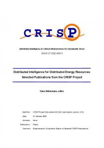
We implemented our algorithm in our Smart Grid simulator [13], which is an innovative integrated framework modelling and simulating both the communication network and power networks, based on OMNeT++ [14]. We simulated three different scenarios in a residential environment. Each scenario simulates a 24 hour period for a neighbourhood of 30 houses with each house having a fixed base load consumption. Figure 4 gives an example of such a base load consumption profile with a peak in the evening and a minimum consumption at night. Each house also has 4 shiftable devices: dryer (4kW for 100 minutes), washing machine (2.5kW for 50 minutes), dishwasher (2.5kW for 140 minutes), boiler (3kW for 70 minutes) and 30% of the houses have an electric vehicle (4kW for 240 minutes). Furthermore, over the different scenarios several renewable energy producers are simulated. To evaluate our MAS algorithm the following metrics were calculated:
800 700 600
Load (W)
500 400 300 200 100 0 0:00
2:00
4:00
6:00
8:00
10:00
12:00
14:00
16:00
18:00
20:00
22:00
Time
•
•
•
•
Example base load profile from [15].
Externally supplied energy EE : The total amount of energy consumed in the neighbourhood, supplied via an external power network. Goal is to minimize this amount and maximize the consumption of locally produced power as much as possible. Peak load on externally supplied power Pmax : The maximum load on the external power network supplying the neighbourhood. This peak load should be as low as possible to avoid problems in the distribution network, such as transformator overloads and avoid or postpone extra network investments by the distribution operator. Flatness of external load σ(P ): The standard deviation of the load profile of the externally supplied power is an indication of the flatness of this load curve. It’s more efficient for the supplier of this power to have a flat load. Self consumption of renewable energy ES : The amount of locally produced energy that is also consumed locally. Primary goal of our approach is to maximize this metric.
A. Scenario 1: Wind Energy 1) Case Setup: In this scenario the simulated neighbourhood contains a local wind turbine with a maximal power of 200kW. The maximum power of the external generator is 250kW. The goal of this scenario is to realize load shifts to let the consumption of power coincide as much as possible with the fluctuating production of the wind turbine. The wind turbine is large enough to satisfy 80% of the peak demand of the neighbourhood. For this scenario we simulate a scaled Gamesa G52 wind turbine [17] which has the characteristics as shown on figure 5. The power curve which models the output power of the turbine in function of the wind speed, can be modelled by a piecewise third order polynomial function [16]: P P P P
=0 v < vcutin = av 3 + bv 2 + cv + d vcutin < v < vmaxpower = Pmax vmaxpower < v < vcutout =0 v > vcutout
(1) with vcutin the minimal wind speed for energy production by the wind turbine, vcutout the maximum wind speed for
Fig. 5. Real and modelled power curves for the Gamesa G52-850kW wind turbine [16].
which the wind turbine can produce power, Pmax the maximal power of the wind turbine and vmaxpower , the minimum wind speed for which the wind turbine generates its maximal power. Wind data 26/12/2010 Ostend, Belgium 14
12
Wind d Speed (m/s)
Fig. 4.
10
8
6
4
2
0 0:00
2:00
4:00
6:00
8:00
10:00
12:00
14:00
16:00
18:00
20:00
22:00
Time
Fig. 6.
Wind speeds for a windy day at Ostend, Belgium from [18]
We use wind data from a rather windy day in Ostend, a city at the Belgian coast having several wind farms in the neighbourhood. The wind profile is shown in figure 6. 2) Results: To evaluate our algorithm we build a reference scenario (REF) where the shiftable devices have a fixed operating time, mostly in the evening, whereas in the market scenario (MARKET) these devices have a large operation interval giving the load shifting agents enough flexibility to determine a good moment to start the devices. These operating times are shown in table I. Figures 7 and 8 show the results of a typical simulation run. Both figures show the total consumption in the neighbourhood, the total production of renewable energy within the neighbourhood, and the energy that is consumed from or injected to the external power grid. Consumption is modeled as positive values and production as negative values. Positive values for the external power grid means that power is injected. Table II shows the results for the defined metrics. We see an important reduction in consumed power from the external power grid, a peak load reduction of almost 50% and a reduction of the standard deviation on the external generator profile. In the reference scenario the load is maximal during the evening as people come home, start cooking, washing,
TABLE I A SSUMED OPERATING TIMES FOR SHIFTABLE DEVICES .
TABLE II R ESULTS FOR THE WIND ENERGY SCENARIO
Device
Start REF
Start MARKET
Explanation
Dryer
22h
[0h - 16h]
Ready when you come home after work.
Washing machine
21h
[0h - 17h30]
Ready when you come home after work.
Water boiler
7h
[0h - 7h10]
Ready for a shower in the morning.
Dishwasher
19h
[20h - 7h]
Ready for breakfast.
PHEV
18h
[18h - 8h]
Ready when you leave for work.
the
EE (kWh) Pmax (kW) σ(P ) (kW) ES
Market Algorithm
Improvement
767.35 237.04 94.72 23%
544.76 122.40 78.46 34%
29% 48% 17% 45%
Remark that our algorithm acts on realtime demand and supply of energy and doesn’t take predictions into account. If the large amount of wind energy during the afternoon could be predicted with a good accuracy, the results could be further improved. 250
External Power Grid (reference)
200
External Power Grid (market algorithm)
150
Reference Scenario
250
Reference
100
Load (kW)
200 150
Load (kW)
100 50 0
50 0
0:00 1:00 2:00 3:00 4:00 5:00 6:00 7:00 8:00 9:00 10:00 11:00 12:00 13:00 14:00 15:00 16:00 17:00 18:00 19:00 20:00 21:00 22:00 23:00 0:00
-‐50
-‐100 0:00 1:00 2:00 3:00 4:00 5:00 6:00 7:00 8:00 9:00 10:00 11:00 12:00 13:00 14:00 15:00 16:00 17:00 18:00 19:00 20:00 21:00 22:00 23:00 0:00
-‐150
-‐50
-‐200
-‐100
-‐250
-‐150
Time
-‐200
External Power Grid
Wind Produc?on
Total Consump?on
Fig. 9. Wind energy scenario: comparison of the load on the external power grid for the reference and market scenarios.
-‐250
Time
Fig. 7.
Wind energy scenario: reference results.
10
Market Equilibrium Price
9 8
Virtual Market Price
charging their car, etc. whereas with the market algorithm the operation of the shiftable devices is postponed to the morning and midday when the virtual market price is low and more wind energy is available. We used a threshold of 50% for the amount of renewable energy in the total production mix for the shiftable devices to encourage the self consumption of green energy. As a result this self consumption rises from 23% to 34%.
7 6 5 4 3 2 1 0
Market Algorithm Scenario
250 200
Fig. 10.
0:00
1:00 2:00
3:00
4:00
5:00 6:00
7:00
8:00
9:00 10:00
11:00
12:00
Time
13:00 14:00
15:00
16:00
17:00 18:00
19:00
20:00
21:00 22:00
23:00
Wind energy scenario: evolution of the market equilibrium price.
150
Load (kW)
100 50 0
0:00 1:00 2:00 3:00 4:00 5:00 6:00 7:00 8:00 9:00 10:00 11:00 12:00 13:00 14:00 15:00 16:00 17:00 18:00 19:00 20:00 21:00 22:00 23:00 0:00
-‐50
-‐100 -‐150 -‐200 -‐250
Fig. 8.
External Power Grid
Wind Produc?on
Total Consump?on
Time
Wind energy scenario: results for the market algorithm.
Figure 9 compares the load on the external power grid for the reference and market scenarios. We see a large reduction of the peak load in the evening and in the morning and around noon less power is injected into the external network, indicating a increase in the self consumption of wind energy. Finally, figure 10 shows the evolution of the market equilibrium price for a typical run of the scenario. Especially in the afternoon the market price is low as renewable production is high and consumption is very low at that moment.
TABLE III R ESULTS FOR THE SOLAR ENERGY SCENARIO
B. Scenario 2: Solar Energy
EE (kWh) Pmax (kW) σ(P ) (kW) ES
Reference
Market Algorithm
Improvement
1033.33 246.50 74.01 19%
8239.84 127.55 52.49 55%
19% 48% 29% 195%
show the results of a typical simulation run. On these figures we see that the high power consumption during the evening is partially shifted towards the middle of the day where abundant solar energy is available. Reference Scenario
250 200 150 100
Load (kW)
1) Case Setup: In this second scenario 50% of the houses have solar panels on the roof of 4kWp each. There is no wind turbine, so the maximal amount of locally produced renewable power is 60kWp. The maximal peak load and corresponding capacity of the external generator is also 250kW. The goal of this scenario is again to maximize the self consumption of the produced solar power. Right now there is often a mismatch between the production and consumption of the power generated by solar panels in residential areas as maximum production is often reached at moments when the inhabitants don’t need a lot of power. For example because they are working during daytime or they are on holiday during the summer. When they arrive at home and start cooking, washing, etc. solar production might be low, especially during the winter. The injection of surplus solar power into the power grid can lead to voltage violations [19]. The production of a solar panel can be modeled by the following equation [20], with A the total surface of the panels (in m2 ), I the irradiance (in W/m2 ), and η the conversion efficiency of the panel:
50 0
0:00 1:00 2:00 3:00 4:00 5:00 6:00 7:00 8:00 9:00 10:00 11:00 12:00 13:00 14:00 15:00 16:00 17:00 18:00 19:00 20:00 21:00 22:00 23:00 0:00
-‐50
-‐100 -‐150
PP V = A × I × η
(2)
-‐200 -‐250
External Power Grid
Solar Energy ProducAon
Total ConsumpAon
Time
Fig. 12.
Solar energy scenario: reference results.
Market Algorithm Scenario
250 200 150 100
Load (kW)
For simplicity reasons we don’t take the conversion efficiency into account, so we assume the solar panels are 100% efficient. The solar radiation or irradiance measures the power of solar radiation per unit area at a surface. The global irradiance is the sum of three terms: the direct irradiance, the diffuse irradiance and the reflected irradiance. The inclination of the PV installation influences the irradiation. We assume a inclination of 35◦ , a southern orientation and use irradiance data for Lisbon in the month December from the Photovoltaic Geographical Information System (PVGIS) [21]. Figure 11 shows the resulting production profile for a 4kWp solar panel.
50 0
0:00 1:00 2:00 3:00 4:00 5:00 6:00 7:00 8:00 9:00 10:00 11:00 12:00 13:00 14:00 15:00 16:00 17:00 18:00 19:00 20:00 21:00 22:00 23:00 0:00
-‐50
-‐100 -‐150
4
-‐200 -‐250
Power (kW)
3
Fig. 13.
External Power Grid
Solar Energy ProducAon
Total ConsumpAon
Time
Solar energy scenario: results for the market algorithm.
2
1
0 0:00
2:00
4:00
6:00
8:00
10:00
12:00
14:00
16:00
18:00
20:00
22:00
Time
Fig. 11. Production profile for a 4kWp solar panel based on the irradiance data for Lisbon in December [21].
2) Results: To evaluate our algorithm we compare again a reference scenario where the shiftable devices have a fixed operating time, with a market scenario where these devices have a large operation interval (see table I). Figures 12 and 13
Table III shows the results for the defined metrics. The amount of power supplied by the external generator is considerably higher than in the wind energy scenario. This is due to the lower production capacity of the solar panels (60kW vs 200kW for the wind turbine) and the fact that the wind turbine can generate power all day long while the solar panels are limited to the period between 8h and 18h. This limited production window is also the reason for the lower reduction in consumed power from the external generator. On the other hand, the peak load reduction is comparable with the wind scenario and the increase in self consumption of renewable energy is considerably higher. The results for the self consumption of green energy are
250
External Power Grid (reference)
200
External Power Grid (market algorithm)
200
150
150 100
50
0:00 1:00 2:00 3:00 4:00 5:00 6:00 7:00 8:00 9:00 10:00 11:00 12:00 13:00 14:00 15:00 16:00 17:00 18:00 19:00 20:00 21:00 22:00 23:00 0:00
-‐50
Load (kW)
Load (kW)
100
0
Reference Scenario
250
50 0
-‐100
-‐100
-‐150
-‐150
-‐200
-‐200
-‐250
0:00 1:00 2:00 3:00 4:00 5:00 6:00 7:00 8:00 9:00 10:00 11:00 12:00 13:00 14:00 15:00 16:00 17:00 18:00 19:00 20:00 21:00 22:00 23:00 0:00
-‐50
External Power Grid
-‐250
Time
Fig. 16.
Neighbourhood scenario: reference results.
Market Algorithm Scenario
250
Market Equilibrium Price
200
9
150
8
100
7
Load (kW)
Virtual Market Price
Total Consump@on
Time
Fig. 14. Sun energy scenario: comparison of the load on the external power grid for the reference and market scenarios. 10
Renewable Produc@on
6 5
50 0
0:00 1:00 2:00 3:00 4:00 5:00 6:00 7:00 8:00 9:00 10:00 11:00 12:00 13:00 14:00 15:00 16:00 17:00 18:00 19:00 20:00 21:00 22:00 23:00 0:00
-‐50
4 -‐100
3
-‐150
2
-‐200
1 0
External Power Grid
Renewable Produc@on
Total Consump@on
-‐250
Time 0:00
1:00 2:00
3:00
4:00
5:00 6:00
7:00
8:00
9:00 10:00
11:00
12:00
13:00 14:00
15:00
16:00
17:00 18:00
19:00
20:00
21:00 22:00
23:00
Time
Fig. 17. Fig. 15.
Neighbourhood scenario: results for the market algorithm.
Sun energy scenario: Evolution of the market equilibrium price.
very good. As already indicated several load shifts occur towards the period during daytime when solar power is available. This is also clearly illustrated in figure 14 comparing the load on the external power grid for the reference and market scenarios. The market equilibrium price, as shown on figure 15, fluctuates a lot during this period. There is a lot of solar power available, so the price is low when the consumption is low. Whenever a load is shifted, the price will rise. The average price over a whole day is higher than for the wind energy scenario due to the lower amount of available renewable energy. C. Scenario 3: Neighbourhood 1) Case Setup: In this third scenario we model a neighbourhood containing both a wind turbine, a number of solar panels and a small storage component. We assume a wind turbine with a production capacity of 150kW, 15 houses with a small solar panel of 1kWp and 1 controllable battery of an electrical car with a energy capacity of 16kWh and maximum charge/discharge capacity of 4.6kW. So the maximal amount of locally produced power is 169.6kW. We use the same wind and irradiance data as in the previous scenarios. 2) Results: Figures 16 and 17 show the results of a typical simulation run for both a reference scenario and a market scenario with the market algorithm.
Table IV shows the results for the defined metrics. The results are a combination of the best elements of the previous scenarios. The reduction of the consumed power from the external generator is comparable with the wind energy scenario and the peak load reduction is comparable with both previous scenarios. The self consumption of green energy is situated between the results of the wind energy and sun energy scenario. The fact that the self consumption is lower than in the sun energy scenario is due to the larger amount of renewable energy that is available. Not all this energy can be consumed by the shiftable devices. D. Evaluation of the historical price strategies In this section we compare the four different price threshold strategies of the load shifting agents for the three presented scenarios. Table V shows the improvements for the different metrics. TABLE IV R ESULTS FOR THE NEIGHBOURHOOD SCENARIO
EE (kWh) Pmax (kW) σ(P ) (kW) ES
Reference
Market Algorithm
Improvement
807.37 239.40 86.67 26%
505.15 120.92 65.63 41%
37% 49% 24% 59%
TABLE V R ESULTS FOR THE HISTORICAL PRICE STRATEGIES
WIND NONE AVERAGE MINMAX 2SIGMA SUN NONE AVERAGE MINMAX 2SIGMA NEIGHBOURHOOD NONE AVERAGE MINMAX 2SIGMA
EE
Pmax
σ(P )
ES
38% 29% 63% 60%
-34% 48% 39% 52%
13% 17% 31% 27%
18% 45% 41% 25%
20% 19% 30% 19%
47% 48% 46% 49%
29% 29% 29% 31%
184% 195% 162% 204%
38% 37% 62% 72%
10% 49% 10% 60%
-42% 24% 26% 38%
26% 59% 31% 36%
For the sun energy scenario, the differences between the different strategies are rather small, but for the two other scenarios there are some notable differences. It’s clear that taking historical information into account is useful as the NONE strategy performs the worst overall. The 2SIGMA strategy performs the best with respect to the reduction of the load on the external power grid whereas the AVERAGE strategy performs very well for the optimization of the self consumption of renewable sources. As the main goal of our approach is the optimization of this self consumption, the AVERAGE strategy was used for the presented scenarios. V. C ONCLUSIONS & F UTURE W ORK In this paper we presented a distributed algorithm for residential energy management in smart grids. A multi-agent system is used where the agents make energy bids on a central market. Based on demand and supply a market equilibrium price is calculated. Renewable and traditional energy sources, basic loads, smart devices, storage systems, etc. can all be modeled by these agents and corresponding bidding functions. Applicability of the developed algorithm is demonstrated for three different scenarios showing a large improvement of the self consumption of renewable sources in the network (e.g. 59% improvement for the most comprehensive neighbourhood scenario) and a corresponding reduction of the average and peak loads for the externally supplied power (e.g. 49% reduction of the peak load for the neighbourhood scenario). With these results problems in the distribution grid caused by the distributed generation of power and the expected increase in power consumption by e.g. electrical cars, such as transformer overloads or voltage and grid instabilities, are less likely to occur. Furthermore transportation losses are reduced. Using strategies based on historical price data the algorithm can be optimized for either the consumption of green energy or reduction of the average and peak loads for externally supplied power. In the future we will evaluate more complex bidding functions and evaluate our algorithm in other scenarios, e.g. containing extra power storage components at the level of in-
dividual houses or at neighbourhood level. This will allow the neighbourhood to further increase the self consumption of locally produced renewable energy and at the same time the variability on the requested external energy will be reduced, increasing the overall grid stability. We will also look at electrical aspects of the power grid such as voltage violations and we will evaluate different weather conditions. Implementation and deployment of the algorithm in real home environments using for example the recent announced Android@Home [22] platform is considered. ACKNOWLEDGMENT K. Mets would like to thank the Agency for Innovation by Science and Technology in Flanders (IWT) for financial support through his Ph.D. grant. C. Develder is partially supported by the Research Foundation - Flanders (FWO - Vlaanderen) as a post-doctoral fellow.
R EFERENCES [1] M. Webb, SMART 2020: enabling the low carbon economy in the information age, a report by The Climate Group on behalf of the Global eSustainability Initiative (GeSI), 2008. [2] K. Mets, T. Verschueren, W. Haerick, C. Develder, and F. De Turck, “Optimizing smart energy control strategies for plug-in hybrid electric vehicle charging,” 2010 IEEEIFIP Network Operations and Management Symposium Workshops, pp. 293–299, 2010. [Online]. Available: http://ieeexplore.ieee.org/lpdocs/epic03/wrapper. htm?arnumber=5486561 [3] J. Lopes, F. Soares, and P. Almeida, “Integration of electric vehicles in the electric power system,” Proceedings of the IEEE, vol. 99, no. 1, pp. 168 –183, jan. 2011. [4] E. Coster, J. Myrzik, B. Kruimer, and W. Kling, “Integration issues of distributed generation in distribution grids,” Proceedings of the IEEE, vol. 99, no. 1, pp. 28 –39, jan. 2011. [5] K. Clement, E. Haesen, and J. Driesen, “Analysis of the impact of plug-in hybrid electric vehicles on the residential distribution grids by using quadratic and dynamic programming,” in Proceedings of 24th International Battery, Hybrid and Fuel Cell Electric Vehicle Symposium & Exhibition (EVS 24), 2009. [6] A. Mohsenian-Rad, V. Wong, J. Jatskevich, R. Schober, and A. LeonGarcia, “Autonomous demand-side management based on gametheoretic energy consumption scheduling for the future smart grid,” Smart Grid, IEEE Transactions on, pp. 320–331, 2010. [7] Y. Guo, J. Li, and G. James, “Evolutionary optimisation of distributed energy resources,” in AI 2005: Advances in Artificial Intelligence, ser. Lecture Notes in Computer Science, S. Zhang and R. Jarvis, Eds. Springer Berlin / Heidelberg, 2005, vol. 3809, pp. 1086–1091. [8] S. McArthur, E. Davidson, V. Catterson, A. Dimeas, N. Hatziargyriou, F. Ponci, and T. Funabashi, “Multi-agent systems for power engineering applications - part i: Concepts, approaches, and technical challenges,” Power Systems, IEEE Transactions on, vol. 22, no. 4, pp. 1743 –1752, nov. 2007. [9] J. K. Kok, C. J. Warmer, and I. G. Kamphuis, “Powermatcher: multiagent control in the electricity infrastructure,” in Proceedings of the fourth international joint conference on Autonomous agents and multiagent systems, ser. AAMAS ’05. New York, NY, USA: ACM, 2005, pp. 75– 82. [Online]. Available: http://doi.acm.org/10.1145/1082473.1082807 [10] H. F. Wedde, S. Lehnhoff, E. Handschin, and O. Krause, “Real-time multi-agent support for decentralized management of electric power,” in Proceedings of the 18th Euromicro Conference on Real-Time Systems. Washington, DC, USA: IEEE Computer Society, 2006, pp. 43–51. [Online]. Available: http://dl.acm.org/citation.cfm?id=1153916.1153935 [11] S. Lamparter, S. Becher, and J.-G. Fischer, “An agent-based market platform for smart grids,” in Proceedings of the 9th International Conference on Autonomous Agents and Multiagent Systems: Industry track, ser. AAMAS ’10. Richland, SC: International Foundation for Autonomous Agents and Multiagent Systems, 2010, pp. 1689–1696. [Online]. Available: http://dl.acm.org/citation.cfm?id=1838194.1838197
[12] Z. Jiang, “Agent-based control framework for distributed energy resources microgrids,” in Proceedings of the IEEE/WIC/ACM international conference on Intelligent Agent Technology, ser. IAT ’06. Washington, DC, USA: IEEE Computer Society, 2006, pp. 646–652. [Online]. Available: http://dx.doi.org/10.1109/IAT.2006.27 [13] K. Mets, T. Verschueren, C. Develder, T. Vandoorn, and L. Vandevelde, “Integrated simulation of power and communication networks for smart grid applications,” in Computer Aided Modeling and Design of Communication Links and Networks (CAMAD), 2011 IEEE 16th International Workshop on, june 2011, pp. 61 –65. [14] A. Varga and R. Hornig, “An overview of the omnet++ simulation environment,” in Proceedings of the 1st international conference on Simulation tools and techniques for communications, networks and systems & workshops, ser. Simutools ’08. ICST, Brussels, Belgium, Belgium: ICST (Institute for Computer Sciences, Social-Informatics and Telecommunications Engineering), 2008, pp. 60:1–60:10. [Online]. Available: http://dl.acm.org/citation.cfm?id=1416222.1416290 [15] Vlaamse Regulator van de Elektriciteits- en Gasmarkt (VREG), “Verbruiksprofielen,” http://www.vreg.be/verbruiksprofielen-0, 2011. [16] A. Niinisto and P. Wirtanen, “Simulation of the management of a micro grid with wind, solar and gas generators.” Master’s thesis, Aalto University School of Science and Technology, October 2009. [17] Gamesa Corp., “Gamesa g52-850kw brochure,” http://www. gamesacorp.com/recursos/doc/productos-servicios/aerogeneradores/ catalogo-gamesa/gamesa-g5x-catalogue-eng.pdf, 2011. [18] FreeMeteo.com, “Belgium weather forecast - hourly weather history for oostende (airport), belgium,” http://freemeteo.com/default.asp?pid= 15&la=1&gid=2789786, 2010. [19] J. Ringelstein, “Decentralized energy management for smart houses - a building block for future’s smart grid.” http://www.smarthouse-smartgrid.eu/fileadmin/templateSHSG/docs/ publications/JGIF2010 Tokio RJ.pdf, 2010, 6th Japan-Germany Industry Forum, Tokio. [20] J. V. Paatero and P. D. Lund, “Effects of large-scale photovoltaic power integration on electricity distribution networks,” Renewable Energy, vol. 32, no. 2, pp. 216 – 234, 2007. [Online]. Available: http://www.sciencedirect.com/science/article/pii/S0960148106000425 [21] European Commission - JRC, “Photovoltaic geographical information system (pvgis),” http://re.jrc.ec.europa.eu/pvgis/apps4/pvest.php. [22] eMeter Corp., “Google enters home energy management market with android@home,” http://www.emeter.com/smart-grid-watch/2011/ google-enters-home-energy-management-market-with-androidhome/.