Distributed Multidimensional Scaling with Adaptive Weighting for Node Localization in Sensor Networks JOSE A. COSTA, NEAL PATWARI and ALFRED O. HERO III University of Michigan, Ann Arbor
Accurate, distributed localization algorithms are needed for a wide variety of wireless sensor network applications. This paper introduces a scalable, distributed weighted-multidimensional scaling (dwMDS) algorithm that adaptively emphasizes the most accurate range measurements and naturally accounts for communication constraints within the sensor network. Each node adaptively chooses a neighborhood of sensors, updates its position estimate by minimizing a local cost function and then passes this update to neighboring sensors. Derived bounds on communication requirements provide insight on the energy efficiency of the proposed distributed method versus a centralized approach. For received signal-strength (RSS) based range measurements, we demonstrate via simulation that location estimates are nearly unbiased with variance close to the Cram´ er-Rao lower bound. Further, RSS and time-of-arrival (TOA) channel measurements are used to demonstrate performance as good as the centralized maximum-likelihood estimator (MLE) in a real-world sensor network. Categories and Subject Descriptors: C.2.4 [Computer-Communication Networks]: Distributed Systems—Distributed applications; I.5.4 [Pattern Recognition]: Applications—Signal processing General Terms: Algorithms, Performance Additional Key Words and Phrases: Distributed optimization, multidimensional scaling, node localization, position estimation, sensor networks
1.
INTRODUCTION
For monitoring and control applications using wireless sensor networks, automatic localization of every sensor in the network will be a key enabling technology. Sensor data must be registered to its physical location to permit deployment of energyefficient routing schemes, source localization algorithms, and distributed compression techniques. Moreover, for applications such as inventory management and manufacturing logistics, localization and tracking of sensors are the primary purposes of the wireless network. For large-scale networks of inexpensive, energyefficient devices, it is not feasible to include GPS capability on every device or to This research was partially supported by the National Science Foundation under ITR grant CCR0325571. Author’s addresses: University of Michigan, EECS Dept., 1301 Beal Avenue, Ann Arbor, MI 48109-2122; emails:
[email protected]; {npatwari, hero}@eecs.umich.edu. Permission to make digital/hard copy of all or part of this material without fee for personal or classroom use provided that the copies are not made or distributed for profit or commercial advantage, the ACM copyright/server notice, the title of the publication, and its date appear, and notice is given that copying is by permission of the ACM, Inc. To copy otherwise, to republish, to post on servers, or to redistribute to lists requires prior specific permission and/or a fee. c 2004 ACM 0000-0000/2004/0000-0001 $5.00 ° ACM Journal Name, Vol. V, No. N, June 2004, Pages 1–23.
2
·
Jose Costa et al.
require a system administrator to manually enter all device coordinates. In this paper, we consider the location estimation problem for which only a small fraction of sensors have a priori coordinate knowledge, and range measurements between many pairs of neighboring sensors permit the estimation of all sensor coordinates. Two major difficulties hinder accurate sensor location estimation: first, accurate range measurements are expensive; and second, centralized estimation becomes impossible as the scale of the network increases. This paper proposes a distributed localization algorithm, based on a weighted version of multidimensional scaling (MDS), which naturally incorporates local communication constraints within the sensor network. Its key features are: (1) A weighted cost function that allows range measurements that are believed to be more accurate to be weighted more heavily. (2) An adaptive neighbor selection method that avoids the biasing effects of selecting neighbors based on noisy range measurements. (3) A majorization method which has the property that each iteration is guaranteed to improve the value of the cost function. Simulation results and experimental channel measurements show that even when using only a small number of range measurements between neighbors and relying on fading-prone RSS, the proposed algorithm can be nearly unbiased with performance close to the Cram´er-Rao lower bound. 1.1
Sensor Localization Requirements
For a network of thousands or even millions of sensors, the large scale precludes centralized location estimation. Sending pair-wise range measurements from each sensor to a single point and then sending back estimated device coordinates would overwhelm the capacity of low-bandwidth sensor networks and waste energy. Decentralized algorithms are vital for limiting communication costs (which are usually much higher than computation costs) as well as for balancing the communication and computational load evenly across the sensors in the network. Furthermore, when a sensor moves, the ability to recalculate location locally rather than globally will result in energy savings which, over time, may dramatically extend the lifetime of the sensor network. Sensor energy is also conserved by limiting transmission power. Since the transmit power impacts the SNR of the range measurement, there is a tradeoff between energy cost and accuracy. There is also a tradeoff between device cost and range accuracy: using ultrawideband (UWB) [Fleming and Kushner 1995; Correal et al. 2003] or hybrid ultrasound/RF techniques [Girod et al. 2002] can achieve accuracies on the order of centimeters, but at the expense of high device and energy cost. Alternatively, very inexpensive wireless devices can measure RF received signal strength (RSS) just by listening to network packet traffic, but range estimates from RSS incur significant errors due to channel fading. All range measurements tend to degrade in accuracy with increasing distance. In particular, RSS-based range measurements experience errors whose variance is proportional to the actual range. Accurate localization algorithms must take into account the range dependence of the ranging variance. ACM Journal Name, Vol. V, No. N, June 2004.
Distributed Multidimensional Scaling with Adaptive Weighting
·
3
Finally, measurement of ranges between every pair of devices would require O(n 2 ) measurements for n sensors. The dwMDS algorithm reduces measurement costs by requiring range measurements only between a small number of neighboring sensors. 1.2
Multidimensional Scaling
The goal of multidimensional scaling is to find a low dimensional representation of a group of objects (e.g., sensor positions), such that the distances between objects fit as well as possible a given set of measured pairwise “dissimilarities” that indicate how dissimilar objects are (e.g., inter-sensor RSS). MDS has found many applications in chemical modeling, economics, sociology, political science and, especially, mathematical psychology and behavioral sciences [Cox and Cox 1994]. More recently, MDS has been used by the machine learning community for manifold learning [Tenenbaum et al. 2000]. In the sensor localization context, MDS can be applied to find a map of sensor positions (in 2-D or 3-D) when dissimilarities are measurements of range obtained, for example, via RSS or TOA. For the last 70 years many approaches to solving the MDS problem have been formulated (see [Cox and Cox 1994] and references therein). On the one hand, when the measured dissimilarities are equal to the true distances between sensors, classical MDS provides a closed formed solution by singular value decomposition of the centered squared dissimilarity matrix (see Section 3). On the other hand, when dissimilarities are measured in noise, other techniques should be used, usually based on iteratively minimizing a loss function between dissimilarities and distances. This framework encompasses techniques such as alternating nonlinear least squares (ALSCAL) [Takane et al. 1977], nonlinear least squares via majorizing functions (SMACOF) [Groenen 1993], nonmetric scaling [Kruskal 1964a; 1964b] or maximum likelihood formulations [Ramsay 1982; Zinnes and MacKay 1983]. Common to all these methods is the need for a central processing unit to gather all the available dissimilarities and perform the function minimization. In contrast, we present a distributed MDS algorithm, which operates by minimizing multiple local loss functions. The local nonlinear least squares problem is solved using quadratic majorizing functions as in SMACOF. Since each local cost distributes additively over the network, each sensor contributes to the minimization of the global MDS loss function. In this way, our algorithm produces a sequence of position estimates with corresponding non-increasing global cost and limited communication between sensors. 1.3
Related Work
Many aspects of the sensor localization problem have been addressed in recent literature. Notably, bounds on estimation performance have been derived for the cases when pair-wise measurements are RSS, TOA, AOA (Angle Of Arrival), or a combination [Moses et al. 2003; Patwari et al. 2003; Catovic and Sahinoglu 2004; Niculescu and Nath 2004]. Furthermore, centralized algorithms based on multidimensional scaling [Shang et al. 2003], convex optimization [Doherty et al. 2001], and maximum-likelihood [Moses et al. 2002] have demonstrated good estimation performance. Research has also demonstrated the feasibility of distributed localization algorithms [Niculescu and Nath 2001; Savvides et al. 2002; Nagpal et al. ˇ 2003; Capkun et al. 2001; Albowicz et al. 2001; Savarese et al. 2001], which are ACM Journal Name, Vol. V, No. N, June 2004.
4
·
Jose Costa et al.
required for scalability and balancing computational costs across large sensor networks. Although using a different formulation than the one proposed here, the following papers also apply MDS-type techniques to sensor localization: — Manifold Learning: Centralized manifold learning techniques are used in [Patwari and Hero III 2004] to estimate sensor locations, without explicit range estimation, in cases where sensor data has correlation structure that is monotone in inter-sensor distance. Nonlinear dimensionality reduction is used to estimate physical location coordinates from the high-dimensional sensor data. The present paper uses direct measurements of range between pairs of neighboring devices to estimate locations. — Plain MDS: In [Shang et al. 2003], devices have connectivity information (whether or not two devices are in range). The distance between two connected nodes is defined to be 1, while the distance between two nodes not in range is set to the number of hops in the shortest path between them (similar to Isomap [Tenenbaum et al. 2000]). The matrix of distances between each pair of devices is used by an MDS algorithm to estimate the coordinates of the devices. Compared to the present paper, this centralized MDS method weights each distance equally. Unlike [Shang et al. 2003], the method proposed here avoids the (usually inaccurate) estimation of distances between out-of-range sensors. — Local MDS: In [Ji and Zha 2004], a local version of MDS is used to compute maps of many local arrangements of nodes. These local maps are pieced together to obtain global maps. This method tends to perform better than the global MDS method when node density is non-uniform, or “holes” in coverage exist. The local calculations allow a distributed implementation, but weights are restricted to be either 0 or 1. The formulation introduced in the present paper removes that restriction, by allowing arbitrary non-negative weights, and naturally bypasses the complex step of fusing the local maps into a global map. Common to most sensor localization methods is the process of selecting sensor neighborhoods for range measurements. Most methods propose using only ranges measured between nearby neighbors, in order to limit communication costs and computational complexity. However, when ranges are measured with noise, the act of choosing neighbors based on these measurements will tend to select devices whose measured distances are shorter than the true distances. This paper addresses this biasing effect and proposes a two-stage neighbor selection process that can be used to unbias location estimates even in high-noise environments. We remark that, to our knowledge, this problem has not been previously considered in the sensor localization literature. 1.4
Outline
The remainder of this paper is organized as follows. Section 2 provides a formal statement of the sensor localization problem considered here. In Section 3 we describe the solution to the classical MDS formulation and discuss its shortcomings in a distributed and sensor network environment. The proposed algorithm is introduced in Section 4. In Section 5 we discuss statistical models for TOA and ACM Journal Name, Vol. V, No. N, June 2004.
Distributed Multidimensional Scaling with Adaptive Weighting
·
5
RSS measurements to show why a weighted MDS solution is important. Section 6 discusses the bias effect associated with using these noisy range measurements to select neighboring devices and proposes a solution. In Section 7 we show results on both simulated measurement data and on measured range data recorded for a 44node sensor network in an indoor office environment. Finally, Section 8 concludes the paper with a discussion about the proposed method, improvements and future work. 2.
PROBLEM STATEMENT
To be specific about sensor localization, we now formally state the estimation problem addressed in this paper. Consider a network of N = n + m devices, living in a D-dimensional space (D = 2 or 3, although the proposed formulation can handle arbitrary D-dimensional D localization, as long as D < N ). Let {xi }N i=1 , xi ∈ R , be the actual vector coordinates of sensors, or, equivalently, define the matrix of coordinates X = [x1 , . . . , xn , xn+1 , . . . , xN ]. The last m sensors (i = n + 1, . . . , N ) have perfect a priori knowledge of their coordinates and are called anchor nodes. The first n sensors (i = 1, . . . , n) have either no knowledge or some imperfect a priori coordinate knowledge and are called unknown-location nodes. Imperfect a priori knowledge about sensor i ≤ n is encoded by parameters ri and xi , where, with accuracy ri , xi is believed to lie around xi . If no such knowledge is available, ri = 0. Summarizing, three distinct sets of sensors can be considered in this formulation based on their a priori information: perfect (i > n), imperfect (i ≤ n, ri > 0), or zero coordinate knowledge (i ≤ n, ri = 0). Note that one or two of these sets might be empty, e.g., no anchor nodes available and/or no prior information on sensors locations. These and other notation used throughout this paper is gathered in Table I. The localization problem we consider is the estimation of the coordinates {x i }ni=1 given the coordinates of the anchor nodes, {xi }N i=n+1 , imperfect a priori knowledge, (t) n {(ri , xi )}i=1 and many pairwise range measurements, {δij }, taken over time t = 1 . . . K. We use the terms ’dissimilarity’ and ’range measurement’ interchangeably, in order to seamlessly merge terms common to MDS and localization literature. The available range measurements (i, j) are some subset of {1 . . . N }2 . We assume that this subset of range measurements results in a connected network; otherwise, each connected subset should be considered individually. The method developed is general enough to adapt to any range measurement method, such as TOA, RSS, or proximity. We focus in particular on RSS-based range measurements, due to its desirability as a low-device cost method, but we also test the method using TOA range measurements in Section 7. 3.
CLASSICAL METRIC SCALING
If we assume that we measure all the pairwise dissimilarities {δij }N i,j=1 between points, and that these correspond to the true Euclidean distances, then q δij = dij = d(xi , xj ) = kxi − xj k = (xi − xj )T (xi − xj ) . (1) By writing the squared distances as d2ij = xTi xi − 2xTi xj + xTj xj , one can recover the matrix of inner products between points in the following way. Defining ACM Journal Name, Vol. V, No. N, June 2004.
6
·
Jose Costa et al.
Notation D N =n+m n m Pij Pthr dthr dR xi X dij , dij (X ) (t) δij (t)
wij δ ij wij S Si (k) xi X (k)
Table I. Symbols used in text and derivations Description Dimensions of location estimates (D = 2 unless noted) Total number of sensors Sensors with imperfect or no a priori coordinate information Sensors with perfect a priori coordinate knowledge (‘anchor’ nodes) Power received (dB) at sensor i transmitted by sensor j Minimum received power for successful reception Distance at which mean received power = Pthr Threshold distance for neighborhood selection Actual coordinate vector of sensor i, i = 1 . . . n + m Actual coordinate matrix, [x1 , . . . , xn+m ] Actual distance between sensors i and j in matrix X Range measured at time t between sensors i and j Weight given to the range measured at time t between sensors i and j Weighted average measured range between sensors i and j Weight given to the average measured range between sensors i and j Global objective function to be minimized Local objective function to be minimized at sensor i = 1 . . . n Estimated coordinates of sensor i at iteration k Estimated coordinate matrix at iteration k
ψ = [xT1 x1 , . . . , xTN xN ]T , the squared distance matrix, D = [d2ij ]N i,j=1 , can now be written as D = ψeT − 2X T X + eψ T , where e is the N -dimensional vector of all ones. Defining H to be the centering operator, I − eeT /N , it follows that B = −H D H = H X T X H .
After multiplication with H, the columns of X T X have zero mean. Now, given B, one can recover matrix X , up to a translation and orthogonal transformation, by 1/2
1/2
X = diag(λ1 , . . . , λD ) U T ,
(2)
where B = U diag(λ1 , . . . , λD ) U T is the singular vale decomposition (SVD) of matrix B (see [Cox and Cox 1994] for details). The above derivation exposes the shortcomings of classical MDS. First, obtaining matrix B requires the knowledge of all the pairwise dissimilarities, a scenario highly unlikely in a dense sensor network due to power and/or bandwidth constraints. Second, due to a lack of any special sparse structure, computing matrix B and its SVD requires that all the dissimilarities be communicated and processed by a central processing unit, a communication-intensive operation in most sensor networks. Finally, (2) assumes that the true distances between points are available. For the realistic case in which range measurements have errors, classical metric scal2 ing minimizes the squared error between the squared distances d2ij and δij (rather than the distances themselves) which tends to amplify the measurement errors, resulting in poor noise performance. ACM Journal Name, Vol. V, No. N, June 2004.
Distributed Multidimensional Scaling with Adaptive Weighting
4.
·
7
DISTRIBUTED WEIGHTED MULTIDIMENSIONAL SCALING
We propose a distributed weighted MDS algorithm (dwMDS) that fits the sensor networks framework of distributed computations and restricted communications and also accounts for measurement errors. 4.1
The dwMDS Cost Function
We minimize the following global cost function (a.k.a. STRESS function [Cox and Cox 1994]): ³ ´2 X X X X (t) (t) (3) S=2 wij δij − dij (X ) + ri kxi − xi k2 . 1≤i≤n i 0 (for some t), it can be viewed as the local cost function at node i. We note that if m = 0 (i.e., no anchor nodes are available) and ri = 0, for all i (i.e., no prior information on the nodes locations), then ∂S/∂xi = 2 ∂Si /∂xi . This implies that the influence of xi on the local cost Si determines its influence on the global cost S. Motivated by this cost structure, we propose an iterative scheme in ACM Journal Name, Vol. V, No. N, June 2004.
8
·
Jose Costa et al.
which each sensor updates its position estimate by minimizing the corresponding local cost function Si , after observing dissimilarities and receiving position estimates from its neighboring nodes. 4.2
Minimizing the dwMDS Cost Function
Unlike classical MDS, no closed form expression exists for the minimum of the cost function S or Si . By assuming that each node has received position estimates from neighboring nodes, we minimize Si = Si (xi ) iteratively using quadratic majorizing functions as in SMACOF (Scaling by MAjorizing a COmplicated Function [Groenen 1993]). This method has the attractive property of generating a sequence of nonincreasing STRESS values. A majorizing function Ti (x, y) of Si (x) is a function Ti : RD × RD → R that satisfies: (i) Si (x) ≤ Ti (x, y) for all y, and (ii) Si (x) = Ti (x, x). This function can then be used to implement an iterative minimization scheme. Starting at an initial condition x0 , the function Ti (x, x0 ) is minimized as a function of x. The newly found minimum, x1 , can then be used to define a new majorizing function Ti (x, x1 ). This process is then repeated until convergence (see [Groenen 1993] for details). The trick is to use a simple majorizing function that can be minimized analytically, e.g., a quadratic function. Following [Groenen 1993], we start by rewriting Si as: Si (xi ) = ηδ2 + η 2 (X ) − 2 ρ(X ) , where ηδ2 =
wij δ ij +
n X
wij d2ij (X ) +
n X
wij δ ij dij (X ) +
j=1 j6=i
η 2 (X ) =
j=1 j6=i
ρ(X ) =
n+m X
n X
2
2
2 wij δ ij ,
(6)
j=n+1 n+m X
j=n+1
j=1 j6=i
2 wij d2ij (X ) + ri kxi − xi k2 ,
n+m X
2 wij δ ij dij (X ) .
(7)
(8)
j=n+1
Term (6) does not depend on xi and term (7) is quadratic in xi . Only term (8) depends on xi through a more complicated (sum of square roots) function. Define Ti (x, y) as: Ti (xi , y i ) = ηδ2 + η 2 (X ) − 2 ρ(X , Y ) ,
(9)
where ρ(X , Y ) =
n X j=1 j6=i
wij
n+m X δ ij δ ij (xi −xj )T (y i −y j )+ 2 wij (xi −xj )T (y i −y j ) . dij (Y ) d (Y ) ij j=n+1
(10) ACM Journal Name, Vol. V, No. N, June 2004.
Distributed Multidimensional Scaling with Adaptive Weighting
·
9
Using the fact that, by Cauchy-Schwarz inequality, dij (X ) =
(xi − xj )T (y i − y j ) dij (X ) dij (Y ) ≥ , dij (Y ) dij (Y )
it is easily seen that Ti majorizes Si . Minimizing Si through a majorizing algorithm is now a simple task of finding the minimum of Ti : ∂Ti (xi , y i ) =0. ∂xi
(11)
An expression for this gradient is given in Appendix A. If X (k) is the matrix whose columns contain the position estimates for all points at iteration k, one can derive an update for the position estimate of node i using equation (11): ´ ³ (k) (k+1) , (12) xi = ai ri xi + X (k) bi where a−1 = i
n X j=1 j6=i
wij +
n+m X
2 wij + ri ,
(13)
j=n+1
(k)
= [b1 , . . . , bn+m ]T is a vector whose entries are given by: £ ¤ bj = wij 1 − δ ij /dij (X (k) ) j ≤ n , j 6= i Pn Pn+m bi = j=1 wij δ ij /dij (X (k) ) + j=n+1 2 wij δ ij /dij (X (k) ) . j6=i£ ¤ j>n bj = 2 w ij 1 − δ ij /dij (X (k) )
and bi
(14)
(t)
As the weights wij can be made nonzero only for a relative neighborhood of node i, only the corresponding entries of vector b will be nonzero, and the update rule for xi will depend only on this neighborhood (as opposed to the whole matrix X (k) ). We remark, that unlike the centralized SMACOF algorithm described in [Groenen 1993], the computation of (12) does not require the evaluation of a n × n Moore-Penrose matrix inverse. 4.3
Algorithm
The proposed algorithm is summarized in Figure 1. We make the following comments: (1) The choice of weighting function wij should reflect the accuracy of measured dissimilarities, such that less accurate measurements are down-weighted in the overall cost function. If a noise measurement model is available, w ij can be tailored to the variance predictions of the model. For example, one might select wij = 1/(c1 δij + c2 )2 if the measurements are Gaussian distributed with standard deviation increasing linearly with the true distances, i.e., σ = c1 dij + c2 . When a reliable model is not available, one can adopt a model-independent adaptive weighting scheme. This is the approach adopted in this paper. Inspired by the weighting frequently used in locally weighted regression methods (LOESS) [Cleveland 1979], ACM Journal Name, Vol. V, No. N, June 2004.
10
·
Jose Costa et al. (t)
(t)
Inputs: {δij }, {wij }, m, {ri }, {xi }, ², initial condition X (0) Initialize: k = 0, S (0) , compute ai from equation (13) repeat k ←k+1 for i = 1 to n (k−1) compute b³i from equation (14) ´ (k)
xi
= ai
(k−1)
ri xi + X (k−1) bi
(k)
compute Si (k−1) (k) S (k) ← S (k) − Si + Si (k) communicate xi to neighbors of node i (i.e., nodes for which wij > 0) communicate S (k) to node i + 1 (mod n) end for until S (k−1) − S (k) < ²
Fig. 1.
Algorithm for decentralized weighted-multidimensional scaling
we propose the following weight assignment: © 2 2ª ½ exp −δij /hi , if δij is measured wij = , 0 , otherwise
(15)
where hi = maxj δij . This choice of wij , which equalizes the (nonzero) weight distribution in all sensors, has robust performance as shown in the experiments reported in Section 7. (2) The question of how to adaptively choose the neighbors of each node (i.e., which weights are made positive) in order to decrease communication costs or improve localization performance is addressed in Section 6. (3) Regarding the initialization of the algorithm, every node requires an initial estimate of its position. This can be done using the algorithms proposed in [Savarese ˇ et al. 2001] or [Capkun et al. 2001]: each node builds its local coordinate system, which is then passed along the network until a rough global map of the network is built. In the experiments reported in Section 7, we found that the algorithm was robust with respect to “rough” initial position estimates. (4) In the description of the algorithm, it was assumed for notational convenience, that the algorithm cycles through the network in an ordered fashion (i.e., messages are passed between nodes in the order 1, 2, . . . , n). However, many other non-cyclic update rules are possible. In particular, one possibility is for (spatial) clusters of sensors to iterate among themselves until their position estimates stabilize. These estimates can then be transmitted to the neighboring clusters, before starting a new iteration step. (5) Although the majorization approach used guarantees a non-increasing sequence of STRESS vales, it may converge to a local minimum of this cost function, instead of the global one, like any gradient search method. This behavior can be alleviated to some extent by using some of the advanced search techniques proposed in [Groenen 1993]. 4.3.1 Computational Complexity and Energy Consumption. Regarding computational complexity, it is easily seen that the algorithm in Figure 1 scales as O(n L), ACM Journal Name, Vol. V, No. N, June 2004.
Distributed Multidimensional Scaling with Adaptive Weighting
·
11
where L is the total number of iterations required until the stopping rule is satisfied. This compares favorably to classical MDS, which requires O(n2 T ) operations, where T is the number of steps required by the Lanczos method to compute the necessary SVD. However, in sensor network applications, far more important than computational complexity, is the amount of communication required by the algorithm, as the energy consumed by a single wireless transmission can far outweigh the energy necessary for local computations. As we are interested in how communication complexity scales with the size of the network, we adopt the model proposed in [Rabbat and Nowak 2004]. In this model, the average total energy used by a general data processing algorithm, as function of the number of nodes n, is given by E(n) = b(n) × h(n) × e(n) , where b(n) is the average number of bits/packets transmitted, h(n) is the average number of hops over which communication occurs, and e(n) is the average amount of energy required to transmit one bit/packet over one hop. For simplicity, we assume, in the following analysis, that the sensors are uniformly distributed over a square or cube of unit side length, for, respectively, a D = 2 or D = 3 dimensional network. The proposed algorithm requires that each node transmits its position estimate to other nodes from which it obtained range measurements. If we assume that a node is able to sense all other nodes within a threshold distance dthr , then the average number of neighbors a node can communicate with is upper bounded by c1 (n − 1) dD thr , where c1 is the volume of the D-dimensional unit sphere (nodes close to the border of the unit square or cube actually have fewer expected neighbors). As this operation occurs for each iteration for every node, an upper bound on the average number of transmitted bits is bdwMDS (n) ≤ O(n2 L dD thr ). Each communication to its neighbors can be made in one hop, so hdwMDS (n) = 1. Thus, the average energy required for communication by the proposed algorithm is: ¡ ¢ EdwMDS (n) ≤ O n2 L dD (16) thr edwMDS (n) .
Notice that edwMDS (n) depends on dthr (in a nonlinear way). We remark that the same bound (16) on energy consumption is also valid for a sensor network with nodes distributed over a uniform grid of side length O(n −1/D ) (see Fig. 3). This scenario makes it easier to compare the proposed method to a centralized algorithm, assuming a multi-hop communication protocol. To simplify the analysis, we consider the threshold distance dthr = O(n−1/D ). In this case, each node communicates only with its immediate neighbors in the uniform grid, making the average hop distance the same in the centralized and distributed case. This implies that the same energy is required to transmit a bit/packet over one hop, i.e., edwMDS (n) = ecentr (n). For dthr = O(n−1/D ), each node will, on the average, receive range measurements from a fixed number of neighborhood nodes, no matter how big the network is. The centralized algorithm must transmit them to a fusion center. After a simple calculation, it can be shown that this results in bcebtr (n) = O(n) bits transmitted. For the uniform grid geometry, a simple calculation shows that the average number of hops from a node to the fusion center is hcentr (n) = O(n1/D ). ACM Journal Name, Vol. V, No. N, June 2004.
12
·
Jose Costa et al.
Finally, we obtain the average energy required by a centralized algorithm, ³ ´ Ecentr (n) = O n1+1/D ecentr (n) .
(17)
Substituting for the assumed dthr in expression (16), we obtain the ratio between energies required by a centralized versus a distributed algorithm, in the uniform grid case: µ 1/D ¶ n Ecentr (n) . (18) =O EdwMDS (n) L
For dense networks of the same size n, and fixing a priori the maximum number of iterations allowed, a centralized algorithm will require an order of n1/D more energy than the proposed distributed algorithm. Note that the costs of the centralized algorithm aren’t evenly distributed - nodes near the fusion center will disproportionately bear the forwarding costs. To conclude this section, we remark that, for D = 2 and dthr = O(n−1/D ),√the proposed algorithm has a transport requirement of O(n2 L dD thr ) × dthr = O( n) bit-meters/sec, which is the same as the transport capacity of a wireless network on a unit area region [Gupta and Kumar 2000]. This suggests that the implementation of the proposed algorithm is pratically feasible, even with more resource aggressive update rules (e.g., parallel updates of all nodes), for a large sensor network. 5.
RANGE MEASUREMENT MODELS
For concreteness, we assume throughout the rest of this paper that range measurements between sensors are obtained either via RSS or TOA or a combination of the two. Both RSS and TOA can be measured via RF or by acoustic media; both media are subject to multipath and fading phenomena which impair range estimates. 5.1
Time-of-Arrival
For a TOA receiver, the objective is to identify the time-of-arrival (TOA) of the direct line-of-sight (DLOS) path.1 The power in the DLOS path is attenuated by any obstacles in between the transmitter and the receiver, and often, later-arriving non-line-of-sight(NLOS) multipath components arrive at the receiver with equal or greater power than the DLOS. As the distance between two devices increases, measurements have shown that the late-arriving paths contribute an increasing proportion of the overall received power [Pahlavan et al. 1998], effectively decreasing the SNR of the TOA measurements, and increasing NLOS range error. Previous research has suggested using weighted least-squares algorithms to improve localization performance [Chen 1999]. 5.2
Received Signal Strength
Similarly, range measurements based on RSS degrade with distance. Objects in the environment between the transmitter and receiver have the effect of multiplying 1 This is a different goal than for a communications receiver, which aims to synchronize to the time which maximizes the SNR, regardless of whether the signal power comes from the DLOS path or later arriving paths.
ACM Journal Name, Vol. V, No. N, June 2004.
Distributed Multidimensional Scaling with Adaptive Weighting
·
13
the signal energy by attenuation factors. The cumulative effect of many such multiplications, by a central limit argument, result in a log-normal distribution of RSS (or equivalently received power) at the receiver [Coulson et al. 1998]. If Pij (mW), the received power in mW at sensor i transmitted by sensor j, is log-normal, then received power in decibels, Pij = 10 log10 Pij (mW), is Gaussian. Furthermore, RF channel measurements have shown that the variance of Pij is largely constant over path length [Rappaport 1996][Patwari et al. 2003]. Thus Pij is typically modeled as 2 Pij ∼ N (P¯ij , σdB ) ¯ Pij = P0 − 10np log10 (dij /d0 )
(19)
δij = d0 10(P0 −Pij )/(10np ) .
(20)
2 where P¯ij is the mean power in decibel milliwatts at distance dij , σdB is the variance of the shadowing, and P0 (dBm) is the received power at a reference distance d0 . Typically d0 = 1 meter, and P0 is calculated from the free space path loss formula [Rappaport 1996]. The path loss exponent np is a parameter determined by the environment. From this model for received power as a function of distance dij , the maximum likelihood estimator of distance is:
If Pij = P¯ij , then δij = dij . When Pij 6= P¯ij , we can see why distance errors increase proportionally with distance. Consider a constant dB error in the received power measurement: ∆ = P¯ij − Pij . For this error, δij = dij 10∆/(10np ) , thus the actual distance is multiplied by a constant factor. In fact, the range estimation error, δij − dij , is directly proportional to dij by the constant factor 10∆/(10np ) − 1. Assuming constant standard deviation σdB of received power with distance, the range estimation error standard deviation will also increase proportionally with distance. This characteristic of RSS-based range estimation leads to very high errors at large path lengths, which have limited its application in traditional location systems. However, in a dense sensor network, the distances between neighboring sensors is small, and a weighted least-squares estimator can be designed to fully utilize the accuracy of the range measurements made between the closest neighbors. 6.
ADAPTIVE NEIGHBORHOOD SELECTION
Typically, neighbors are selected by choosing those devices which are closer than a threshold distance. But, since the exact distance is not known, we need to use noisy measurements to select neighbors. Range measurements, whether made via TOA, RSS, or proximity, are all subject to errors. In this section we discuss the biasing effects of selecting neighbors via noisy distance measurements, and how we can unbias the selection. When distance is measured in noise, the act of thresholding neighbors based on the measured distance will tend to select the devices with smaller measured distances. For example, consider two devices separated by distance R, when R is also the threshold distance. With some positive probability (due to noise), the measured distance, δ, will be greater than R, and the two will not be considered ACM Journal Name, Vol. V, No. N, June 2004.
14
·
Jose Costa et al.
neighbors. Alternatively, if δ ≤ R, the two will be considered neighbors, and δ will be used in the localization algorithm. The problem is that the expected value of δ, for devices separated by R which consider themselves neighbors, is less than R. Thus, the measured distance is negatively biased because of the effect of thresholding. Note that selecting the K-nearest-neighbors effectively has an adaptive threshold, and thus does not avoid this biasing effect. This bias has not been specifically addressed in the sensor localization literature, because its effects are not severe in certain systems. Some proposed sensor localization systems measure very accurate distances, eg., using TOA in UWB or a combination of RF and ultrasound media – for these systems, the effect of selecting neighbors based on measured distances will be minimal. Alternatively, if neighbors are selected based an independent means (eg., based on RSS or connectivity when range estimates are based on TOA), than the biasing effect is avoided 2 . Finally, when studies show results for the case in which all devices are connected to every other device, the thresholding step (and its biasing effect) is eliminated. In this paper, we consider both noisy RSS measurements and small neighborhoods, so we cannot avoid the biasing effect. We limit our discussion to RSS measurements in this section, since low device costs and energy consumption are very attractive device characteristics of RSS, but the discussion is also applicable to systems which use noisy TOA-based range measurements for neighbor selection. 6.1
RSS-based Biasing Effect
When discussing thresholding based on RSS, we must make a distinction between the physical limits of the receiver and the threshold which we use to select neighbors, because generally, the two do not need to be the same. If a device has a large radio range to be robust to low device densities, it may want a stricter threshold when there are very many devices with which it can communicate. Denote Pthr to be the received power level below which a receiver cannot demodulate packets. (For most digital receivers with large frames and FEC, the frame error rate is very close to zero or very close to one for the vast majority of SNR, and the transition region is narrow. Thus, to a good approximation, for a constant noise level, we can state that packets above Pthr are received and demodulated correctly, while those below are not [Patwari and Hero III 2003].) Denote PR to be the received power level below which we do not include the transmitting device as a neighbor. Clearly, PR ≥ Pthr . Equivalently, we can define distances dthr and dR from (19) to be the range at which the mean received power is equal to Pthr and PR , respectively. Whether or not we select neighbors based on connectivity (measured power is greater than Pthr ) or select them based on a power threshold (measured power is greater than PR ), the biasing effect will be the same. In following, we use PR and dR to indicate the thresholds (which may be set equal to Pthr and dthr if desired). Let E [δij |Pij > PR ] be the expected value of the range estimate between devices i and j given that the two are neighbors (i.e., the received power Pij is greater than 2 Note, however, for the RSS/TOA example, that if both are available, we may wish to use a combination of both; and if not, RSS and TOA for a link are correlated because objects in the environment tend to degrade both measurements simultaneously.
ACM Journal Name, Vol. V, No. N, June 2004.
Distributed Multidimensional Scaling with Adaptive Weighting
·
15
E[dMLE/dthr | Rx Power > Pthr]
1
0.8
0.6
0.4
0.2 RSS Ideal 0 0
0.5 1 1.5 2 Actual Distance Ratio: d
actual
2.5
3
/d
thr
Fig. 2. The expected value of the RSS-based estimate of range given that that two devices are neighbors (- - -), and the ideal unbiased performance (—). The channel has σ dB /n = 1.7 and dR = 1 (or equivalently, distances are normalized by dR ).
PR ). Using the RSS measurement model (see Section 5.2), it can be shown that ³√ ´ kx −x k 1−Φ β log idR j + √1β ´ ³√ E [δij |Pij > PR ] = kxi − xj k C , (21) kx −x k 1−Φ β log idR j where Φ(.) is the cumulative distribution ³ ´ function of a standard Gaussian random 10np 1 variable, β = σdB log 10 , C = exp 2β 2 and σdB , np are channel parameters. Equation (21) is plotted in Fig. 2 as a function of the ratio of the true distance to d R . Ideally, the range estimator should have a mean value equal to the actual range. However, as the range increases, the expected value of δij (given that i and j are neighbors) deviates from linear and asymptotically becomes constant. There is a strong negative bias for devices separated by dR or greater. 6.2
Neighborhood Prediction
Motivated by the negative bias phenomenon displayed in Fig. 2, we propose a two stage neighborhood selection process, based on the predicted distances between sensors. In the first step, the dwMDS algorithm from Fig. 1 is run with a neighborhood structure based on the available range measurements, i.e., set wij = 0 if δij > ˆ i } of the sensors dR . After convergence, this step provides an interim estimate {x locations. With high probability, the predicted distances between the estimated sensor locations will be negatively biased. In the second step, these predicted distances from the estimated sensor locations are used to compute a new neighborhood structure, by assigning wij = 0 if kˆ xi − ˆ j k > dR . Some neighbors with low range measurements will be dropped, and some x ˆ i} neighbors with possibly longer range measurements will be added. Then, using { x as an initial condition and the new neighborhood structure, the dwMDS algorithm ACM Journal Name, Vol. V, No. N, June 2004.
16
·
Jose Costa et al.
is re-run, resulting in the final location estimates. Note that the predicted distances ˆ j k are used only to select neighbors (i.e., which weights are positive) – the kˆ xi − x measured ranges δij are still used to determine the weight values. We remark that this 2-step algorithm does not imply twice the computation. The dwMDS algorithm is based on majorization, and each iteration brings it closer to convergence. Since the first step only needs to provide coarse localization information, it does not need to be very accurate, and so the dwMDS algorithm can be stopped quickly with a large ². Next, the second step begins with very good (although biased) coordinate estimates, so the second run of the dwMDS algorithm will likely require fewer iterations to converge. Note that for some of the devices which are considered neighbors in the 2nd run of the algorithm, the measured range δij will actually be greater than dR . Thus, to use this 2-step algorithm, dR must be sufficiently less than the physical communication limit of the devices, dthr , so that other range measurements can be considered. If we consider the non-circular (real-world) coverage area of a device, dthr can be considered to be the mean radius of the coverage area, while dR should be set to the minimum radius of the coverage area. 7.
EXPERIMENTAL LOCALIZATION RESULTS
We apply the proposed MDS algorithm to the location problem in a network, using both simulated data and real data collected on an experimental sensor network. 7.1
Simulations
In this section, all the simulated data were generated from the RSS measurement model presented in Section 5.2, with channel parameters σdB /np = 1.7. We first demonstrate the performance of the proposed algorithms on a network of 7 × 7 sensors arranged on a uniform grid of unit area, in which the four corner devices are anchor nodes and the remaining 45 are unknown location devices. For all experiments on this configuration, we use dR = 0.4 m (yielding an average of 14 neighbors per device). We ran 200 Monte Carlo simulation trials to determine confidence ellipses, root-mean-square error (RMSE) and bias performance (per sensor) of the location estimates. The results are displayed in Figure 3, where we plot the mean and 1-σ uncertainty ellipse of the estimator, and compare it to the actual device location and the Cram´er-Rao lower bound (CRB) on the uncertainty ellipses [Patwari et al. 2003]. We remark that the CRB shown is calculated assuming full connectivity (all devices measure range to all other devices), and as such provides only a loose lower bound on the best performance achievable by any unbiased estimator. In the first experiment, we provide a baseline best-case scenario by using perfect (noise-free) distance measurements to select neighborhoods. The baseline assumes that we have an oracle to tell us when the true distance between i and j is less than a threshold, ie., kxi − xj k < dR . This is shown in Figure 3(a), resulting in a RMSE of the location estimates of 0.090 m and an average bias of 0.019 m. For the second experiment, we remove the assumption of perfect connectivity knowledge. Instead, we use RSS measurements to select neighbors, i.e., devices i and j are neighbors if Pij ≥ PR , or, equivalently, if δij ≤ dR . The results are shown in Figure 3(b). The estimates are strongly pulled towards the center of the square, due to the negative bias of the range estimates which are ‘selected’ by the ACM Journal Name, Vol. V, No. N, June 2004.
Distributed Multidimensional Scaling with Adaptive Weighting
1
1
.833
.833
.667
.667
.5
.5
.333
.333
.167
.167
0
0 0 .167 .333 .5 .667 .833 1
·
17
0 .167 .333 .5 .667 .833 1
(a) neighborhood selection using actual distances (b) neighborhood selection using measured ranges
1 .833 .667 .5 .333 .167 0 0 .167 .333 .5 .667 .833 1 (c) adaptive neighborhood selection Fig. 3. Estimator mean (H) and 1-σ uncertainty ellipse (—) for each blindfolded sensor compared to the true location (·) and CRB on the 1-σ uncertainty ellipse (- - -).
connectivity condition. Now, the RMSE is 0.162 m and the bias is 0.130 m. A third experiment uses the adaptive neighborhood selection method proposed in Section 6.2. The results are displayed in Figure 3(c), where it can be seen that this method succeeds in removing the negative bias effect. The bias has gone back down to 0.012 m, while the RMSE is 0.092m, just slightly higher than the baseline experiment using the oracle. Comparing Figure 3(c) and 3(a), the localization errors of the two-step algorithm are spread more evenly throughout the network compared to the first experiment – the errors for edge devices are reduced, while those in the center have increased. Based on the similarity of the RMSE in both experiments, we believe that the 2-step ACM Journal Name, Vol. V, No. N, June 2004.
18
·
Jose Costa et al. 0.13
RMS Location Error
0.12
0.11
0.1
0.09
0.08
0.4
0.6 0.8 1 Threshold Distance d
1.2
R
Fig. 4. RMSE versus threshold distance for the 7 × 7 uniform grid example using adaptive neighborhood selection.
process eliminates most of the neighbor selection bias. Additionally, by changing the neighbor lists (and therefore the weights) and re-running the dwMDS algorithm, the 2nd iteration also provides the opportunity to break out local maxima, which are more likely to affect edge devices. Finally, the low variance achieved by the 2stage algorithm is very close to the CRB which no unbiased location estimator can outperform, despite the fact that the CRB is an optimistic bound for the scenario considered here. We also studied the influence of the threshold distance on the RMSE performance of the proposed algorithms. Figure 4 shows a plot of the RMSE vs. threshold distance, for the 7 × 7 uniform grid example using adaptive neighborhood selection. It can be seen that there is an optimal threshold distance, dR = 0.5 m, beyond which, no performance increase occurs. As dR is increased beyond this optimal value, more distant sensors are included in the cost function. By the RSS measurement model, the accuracy of range measurements degrades quickly with distance, thus adding these far way sensors will not bring any gain to the estimation algorithm. 7.2
Localization in a Measured Network
To test the performance of the proposed algorithm on real-world channel measurements, we used the RSS and TOA measurements presented in [Patwari et al. 2003]. This data set includes the RSS and TOA range measurements from a network of 44 devices (4 of which are anchor nodes) using a wideband direct-sequence spreadspectrum (DS-SS) transmitter and receiver pair operating at a center frequency of 2.4 GHz. The measurements were made in an open plan office building, within a 14 m square area. The RSS between each pair of devices was measured 10 times, from which the average was calculated and labeled as Pij , for each pair (i, j). We use the bias-corrected MLE to estimate range from the RSS, i.e., δij =
d0 (P0 −Pij )/(10np ) 10 . C
ACM Journal Name, Vol. V, No. N, June 2004.
(22)
Distributed Multidimensional Scaling with Adaptive Weighting
·
19
15
Distance Estimate Error (m)
Data 1−σ window 10
5
0
−5
−10 0
5
10 Distance (m)
15
Fig. 5. Plot of distance measurement errors Vs. distance. The 1 − σ interval superimposed on the ¡ ¢ plot was obtained from the ML fit of the error measurement model N (dij , a dij + b)2 .
We choose to divide by C in (22) because this estimator, as opposed to the MLE in (20), is unbiased, ie., E[δij ] = dij . See [Patwari et al. 2003] for details. To give the reader a feeling of how challenging is to to do sensor localization using RSS range measurements in a real live scenario, we plot, in Figure 5, the error between range measurements and real distances, i.e., δij − dij . Note that the standard deviation of the RSS-based range estimator error increases steadily with distance. But, most importantly, the error as a percentage of actual range is often high: there are several range errors larger than 100% of the actual range. We compare the performance of the dwMDS algorithm with adaptive neighborhood selection to classical MDS and the MLE based solutions from [Patwari et al. 2003]. Figures 6(a) and 6(b) show the location estimates using classical MDS (which used all the pairwise range measurements between sensors) and the dwMDS algorithm, for the RSS measurement data set. The true and estimated sensor positions are marked by ’o’ and ’O’, respectively, where the lines represent the estimation errors. The anchor nodes are marked with an ’x’. It can be observed that the dwMDS algorithm does much better than classical MDS. In fact, the RMSE for the classical MDS solution is 4.301 m, while for dwMDS, using dR = 6 m (yielding an average of 19 neighbors per sensor), it drops to 2.477 m. This error is slightly higher than the RMSE of 2.18 m reported in [Patwari et al. 2003], using a centralized MLE. However, that method not only uses all pairwise range measurements, but also relies on previously estimating the channel parameters. If we allow d R to increase at the expense of increasing communication costs, the dwMDS algorithm can reach an RMSE as low as 2.269 m for dR = 8.5 m. Figure 6(c) and 6(d) shows again the location estimates using classical MDS and the dwMDS algorithm, but this time for the TOA measurement data set. The RMSE for the classical MDS solution is 1.959 m and 1.117 m for the dwMDS algorithm using dR = 6 m (wich yields an average of 17.5 neighbors per sensor). This error is slightly better than the RMSE of 1.23 m reported in [Patwari et al. ACM Journal Name, Vol. V, No. N, June 2004.
20 15
·
Jose Costa et al. 15
10
10
5
5
0
0
−5
−5
−5
0
5
10
15
−5
(a) Classical MDS (RSS)
15
10
10
5
5
0
0
−5
−5 0
5
10
5
10
15
(b) dwMDS (RSS)
15
−5
0
15
(c) Classical MDS (TOA)
−5
0
5
10
15
(d) dwMDS (TOA)
Fig. 6. Location estimates using RSS and TOA range measurements from experimental sensor network. True and estimated sensor locations are marked, respectively, by ’o’ and ’O’, while anchor nodes are marked by ’x’. The dwMDS algorithm uses adaptive neighbor selection, with d R = 6 m.
2003], using a centralized MLE. If we allow dR to increase at the expense of increasing communication costs, the dwMDS algorithm can reach an RMSE as low as 0.940 m for dR = 7.5 m. Once again, we stress that the dwMDS algorithm, unlike the MLE estimator from [Patwari et al. 2003], does not use all the pairwise range measurements and doesn’t assume knowledge of the distribution of the range measurements. 8.
CONCLUSION
This paper proposes a distributed weighted-MDS method specially suited for node localization in a wireless sensor network. First, the method reflects the distributed nature of the problem, incorporating network communication constraints in its ACM Journal Name, Vol. V, No. N, June 2004.
Distributed Multidimensional Scaling with Adaptive Weighting
·
21
design. In this way, the need to transmit all range measurements to a central unit is eliminated, resulting in energy savings for a dense sensor network. Second, the inhomogeneous character of range measurements in a wireless network is accounted for by introducing weights that adaptively emphasize measurements believed to be more accurate. We stress that the dwMDS algorithm is nonparametric in its nature, i.e., it does not depend on any particular channel or range measurement models. This makes it applicable to a broad range of distance measurements, e.g., RSS, TOA, proximity, without the need to tweak any parameters. We have shown via simulation that the algorithm has excellent bias and variance performance compared to the CRB, and that its performance in a real-world sensor network is similar to the centralized MLE algorithm. We remark that the dwMDS algorithm can be applied more generally to dimensionality reduction problems across a network of processors, such as internet monitoring or distributed sensor data compression. To make it more general, other distance metrics can be used, such as Lp (1 ≤ p ≤ 2) metrics. In this case, a majorization technique can still be used which guarantees a non-increasing cost function. For other general distances (without any convex structure), gradient descent techniques can be used. In particular, incremental gradient methods fit well the framework considered in this paper and might provide faster convergence rates at the cost of losing the monotonicity of the cost function. A.
APPENDIX
In this appendix, we give an expression for the gradient of the majorizing function Ti defined by equation (9). n n+m n+m n X X X X 1 ∂Ti (xi , y i ) = w + w + r w x − 2 2 wij xj x − ij ij i i ij j 2 ∂xi j=1 j=n+1 j=n+1 j=1 j6=i
j6=i
− r i xi − +
n X j=1 j6=i
wij
n X j=1 j6=i
wij
n+m X
δ ij δ ij y 2 wij + dij (Y ) j=n+1 dij (Y ) i
n+m X δ ij δ ij 2 wij yj + y . dij (Y ) d (Y ) j ij j=n+1
(23) REFERENCES Albowicz, J., Chen, A., and Zhang, L. 2001. Recursive position estimation in sensor networks. In IEEE Int. Conf. on Network Protocols. 35–41. Catovic, A. and Sahinoglu, Z. 2004. The cramer-rao bounds of hybrid toa/rss and tdoa/rss location estimation schemes. Tech. Rep. TR2003-143, Mitsubishi Electric Research Laboratory. Jan. Chen, P.-C. 1999. A non-line-of-sight error mitigation algorithm in location estimation. In IEEE Wireless Comm. and Networking Conf. 316–320. ACM Journal Name, Vol. V, No. N, June 2004.
22
·
Jose Costa et al.
Cleveland, W. 1979. Robust locally weighted regression and smoothing scatterplots. Jornal of the American Statistical Association 74, 368, 829–836. Correal, N. S., Kyperountas, S., Shi, Q., and Welborn, M. 2003. An ultra wideband relative location system. In IEEE Conf. on Ultra Wideband Systems and Technologies. Coulson, A. J., Williamson, A. G., and Vaughan, R. G. 1998. A statistical basis for lognormal shadowing effects in multipath fading channels. IEEE Trans. on Veh. Tech. 46, 4 (April), 494– 502. Cox, T. and Cox, M. 1994. Multidimensional Scaling. Chapman & Hall, London. Doherty, L., pister, K. S. J., and Ghaoui, L. E. 2001. Convex position estimation in wireless sensor networks. In IEEE INFOCOM. Vol. 3. 1655 –1663. Fleming, R. and Kushner, C. 1995. Low-power, miniature, distributed position location and communication devices using ultra-wideband, nonsinusoidal communication technology. Tech. rep., Aetherwire Inc., Semi-Annual Technical Report, ARPA Contract J-FBI-94-058. July. Girod, L., Bychkovskiy, V., Elson, J., and Estrin, D. 2002. Locating tiny sensors in time and space: a case study. In IEEE Int. Conf. on Computer Design. 214–219. Groenen, P. 1993. The majorization approach to multidimensional scaling: some problems and extensions. DSWO Press, Leiden University. Gupta, P. and Kumar, P. R. 2000. The capacity of wireless networks. IEEE Trans. on Inform. Theory 46, 2, 388–404. Ji, X. and Zha, H. 2004. Sensor positioning in wireless ad-hoc sensor networks with multidimensional scaling. In IEEE INFOCOM (to appear). Kruskal, J. 1964a. Multidimensional scaling by optmizing goodness-of-fit to a nonmetric hypothesis. Psychometrika 29, 1–27. Kruskal, J. 1964b. Nonmetric multidimensional scaling: a numerical method. Psychometrika 29, 115–129. Moses, R. L., Krishnamurthy, D., and Patterson, R. 2002. An auto-calibration method for unattended ground sensors. In Proc. of IEEE Int. Conf. on Acoust. Speech and Signal Processing. Vol. 3. 2941–2944. Moses, R. L., Krishnamurthy, D., and Patterson, R. 2003. A self-localization method for wireless sensor networks. EURASIP Journal on Applied Sig. Proc. 4 (Mar.), 348–358. Nagpal, R., Shrobe, H., and Bachrach, J. 2003. Organizing a global coordinate system from local information on an ad hoc sensor network. In 2nd Intl. Workshop on Inform. Proc. in Sensor Networks. Niculescu, D. and Nath, B. 2001. Ad hoc positioning system. In IEEE Globecom 2001. Vol. 5. 2926 –2931. Niculescu, D. and Nath, B. 2004. Error characteristics of ad hoc positioning systems. In ACM MOBIHOC. Pahlavan, K., Krishnamurthy, P., and Beneat, J. 1998. Wideband radio propagation modeling for indoor geolocation applications. IEEE Comm. Magazine, 60–65. Patwari, N. and Hero III, A. O. 2003. Using proximity and quantized RSS for sensor localization in wireless networks. In IEEE/ACM 2nd Workshop on Wireless Sensor Nets. & Applications. Patwari, N. and Hero III, A. O. 2004. Manifold learning algorithms for localization in wireless sensor networks. In Proc. of IEEE Int. Conf. on Acoust. Speech and Signal Processing. Patwari, N., Hero III, A. O., Perkins, M., Correal, N., and O’Dea, R. J. 2003. Relative location estimation in wireless sensor networks. IEEE Trans. Sig. Proc. 51, 8 (Aug.), 2137–2148. Rabbat, M. and Nowak, R. 2004. Distributed optimization in sensor networks. In 3rd Int. Symp. on Information Processing in Sensor Networks (IPSN’04). Berkeley, CA. Ramsay, J. 1982. Some statiscal approaches to multidimensional scaling data. J. R. Statist. Soc. A 145, part 3, 285–312. Rappaport, T. S. 1996. Wireless Communications: Principles and Practice. Prentice-Hall Inc., New Jersey. ACM Journal Name, Vol. V, No. N, June 2004.
Distributed Multidimensional Scaling with Adaptive Weighting
·
23
Savarese, C., Rabaey, J. M., and Beutel, J. 2001. Locationing in distributed ad-hoc wireless sensor networks. In Proc. of IEEE Int. Conf. on Acoust. Speech and Signal Processing. 2037– 2040. Savvides, A., Park, H., and Srivastava, M. B. 2002. The bits and flops of the n-hop multilateration primitive for node localization problems. In Intl. Workshop on Sensor Nets. & Apps. 112–121. Shang, Y., Ruml, W., Zhang, Y., and Fromherz, M. P. J. 2003. Localization from mere connectivity. In Proc. of the 4th ACM Int. Symp. on Mobile Ad Hoc Networking & Computing. 201–212. Takane, Y., Young, F., and de Leeuw, J. 1977. Nonmetric individual differences multidimensional scaling: an alternating least squares method with optimal scaling features. Psychometrika 42, 7–67. Tenenbaum, J. B., de Silva, V., and Langford, J. C. 2000. A global geometric framework for nonlinear dimensionality reduction. Science 290, 2319–2323. ˇ Capkun, S., Hamdi, M., and Hubaux, J.-P. 2001. GPS-free positioning in mobile ad-hoc networks. In 34th IEEE Hawaii Int. Conf. on System Sciences (HICSS-34). Zinnes, J. and MacKay, D. 1983. Probabilistic multidimensional scaling: complete and incomplete data. Psychometrika 48, 27–48. Submitted to ACM Transactions on Sensor Networks June 2004
ACM Journal Name, Vol. V, No. N, June 2004.