Section 2 presents a brief overview of the major concepts of Scopes and the ..... (Note that RtM was sampled every 2 seconds, thus the theoretical goodput is 30.
Distributed Network Structuring with Scopes Daniel Jacobi† , Pablo E. Guerrero† , Ilia Petrov† , and Alejandro Buchmann Databases and Distributed Systems Group, Dept. of Computer Science, Technische Universit¨ at Darmstadt, Germany {jacobi,guerrero,petrov,buchmann}@dvs.tu-darmstadt.de http://www.dvs.tu-darmstadt.de
Abstract. Traditionally, wireless sensor networks were based on the assumption that all sensor nodes are participating in a single global application. However, it is desirable to use sensor networks for multiple concurrent applications. A key factor is the ability to dynamically structure the network into groups of nodes according to certain criteria, to later interact with the group as a whole. In this paper we present Scopes, a modular framework to support concurrent sensor network applications. A scope is a programming abstraction to declaratively define groups, which once established allow data exchange among scope members. The main challenges in attaining these goals are network dynamics such as variable node density, topology changes and node churn. We demonstrate the feasibility of the concept by achieving rapid scope propagation, high scope reliability and efficient data exchange.
1
Introduction
Traditionally, the instrumentation of an environment with a wireless sensing and control infrastructure has been realized with one particular application in mind. Scenarios such as home, building and industrial automation, however, all face the need to exploit the installed resources for multiple, concurrent applications [1,2]. Consider for instance a smart building, where applications such as HVAC control, motion sensing for light switching, and fire detection could all run simultaneously, simplifying the infrastructure. Established architectures such as ZigBee’s, and the support for multiple modules [3] and multithreading [4] indeed allow nodelevel concurrency. We argue that these solutions fall short in offering a clear network-level mechanism to exploit resources when multiple applications run concurrently, leaving the developer with the responsibility of selecting the subset of network nodes on which applications run. Another shortcoming of current systems is their management. The large and dynamic amount of devices that comprise the wireless network make prevalent node classifications such as coordinator/router/end-device in many cases † Parts of this research have been supported by the German Research Foundation (DFG) within the research training group 1362 Cooperative, Adaptive, and Responsive Monitoring in Mixed Mode Environments, and the Center for Advanced Security Research Darmstadt (CASED).
2
D. Jacobi, P. Guerrero, I. Petrov, and A. Buchmann
insufficient for the development of distributed sensor network applications. Several solutions facilitate manageability through the intuitive idea of node groups [5,6,7,8,2]. A group’s extent has a direct implication on its energy cost. Onehop neighborhoods are the cheapest by exploiting the broadcast mechanism [5]. Multi-hop groups covering larger network regions have also prooved useful [6,8]. We think that creating logical groups spanning nodes which are potentially scattered throughout the whole network is important for many applications. In this work we present Scopes, a framework that tackles the aforementioned issues. We show its feasibility through real-world experiments on a sensor network testbed. A scope is simply a group of nodes defined by a set of criteria. Scoping criteria are defined declaratively and are logical predicates on static or dynamic attributes. Of importance for this approach is the rapidness with which a scope definition is propagated and becomes functional, the reliability in covering all nodes meeting a scopes criteria, and the stability against network dynamics. We obtain very good results for all three aspects. Scopes are automatically maintained by the framework, coping with network changes. Once created, a scope enables a bidirectional communication between the scope’s creator and its members. We analyze the goodput and link-level message exchange for both directions and different traffic patterns. Our measurements show good channel utilization, particularly up to an order of magnitude improvement over the baseline routing protocol for traffic originating from member nodes. Section 2 presents a brief overview of the major concepts of Scopes and the framework design. Section 3 contains the detailed evaluation of Scopes according to the above mentioned aspects. We conclude the paper by presenting related approaches (Section 4) and our major findings (Section 5).
2
The Scopes Framework
Scopes is a modular framework that enables multitasking by bringing a logical structure to the network. With the Scopes framework, nodes are organized into groups, which we call scopes (to distinguish we will use the lower and upper case form throughout the document). A scope is the central abstraction provided by the framework to applications. A scope can be defined by means of a logical expression, which must be satisfied by a node to become its member. Once a scope is created, it continues to exist until it is explicitly removed, even as nodes fail or if they temporarily leave and rejoin. The framework takes care of reliably maintaining the scope membership. We have designed a declarative language to create and delete scopes1 . We exemplify the most important constructs within the building automation scenario above, shown in Table 1. Imagine we want to define a scope HVAC Outlier over HVAC equipment nodes not within room temperature limits, so that the heating output can be adjusted. An application running on this scope reports 1
For space reasons, we do not fully describe the Scopes language syntax in this paper. The reader is referred to the project site, www.dvs.tu-darmstadt.de/research/scopes, for a detailed description.
Distributed Network Structuring with Scopes
3
the id and position of the member nodes. HVAC Outlier is satisfiable by nodes with a temperature sensor, whose temperature is outside the range (20. . .25), and the user-defined variable ATTACHED TO equals hvac. Properties included in an expression may have a more static (e.g., ATTACHED TO) or dynamic (e.g., TEMPERATURE) nature. Dynamic properties are very powerful, but their use is expensive since every change results in a re-evaluation of the scope membership expression. Finally, scopes can be nested and therefore form a hierarchy. Nested scopes specialize a scope definition by implicitly restricting the membership condition of their parent-scope. For example, if a scope Room22 is defined over all nodes in room 22, the scope Room22MotionNodes could specialize it by selecting those nodes additionally possessing a motion sensor. The latter can then be used to detect motion and switch lights correspondingly. Every scope has a parent-scope; top-level scopes have an artificial parent-scope called world, which includes all available nodes. A node that does not belong to any scope is member of the world. Conceptually speaking, nesting scopes contributes clearer definitions and better organization. Technically, they reduce the communication overhead thus improving the performance and the energy efficiency.
CREATE SCOPE HVAC_Outlier AS ( ATTACHED_TO = ‘hvac’ AND EXISTS SENSOR TEMPERATURE AND (TEMPERATURE = 25) );
CREATE SCOPE Room22MotionNodes ( EXISTS SENSOR Motion ) AS SUBSCOPE OF Room22;
Table 1: Scope declarative definitions
External (i.e. out-of-network) applications can resort to this language to create scopes. Such expressions are parsed and flattened into a pre-order network format specifically designed for sensor networks. This format is descriptive enough to accommodate the necessary expressions, yet compact enough to typically fit in one network message. Scope creation requests are then handed over to a node, e.g., over a serial port. In-network applications can also construct scopes by resorting to this predefined format. Any arbitrary node can be used to create a scope (termed the scope root node), however in practice we observe two cases. Scopes created from gateway (sink) nodes have global and permanent character. Regular nodes in most cases create localized neighborhood scopes for tasks such as event detection. Scopes enable a bidirectional communication channel between the member nodes and their root node. The framework can operate with multiple routing algorithms. Any routing algorithm supporting bidirectional traffic and multiple concurrent routes can be used. Each top-level scope can be dynamically configured to use any routing algorithm; subscopes inherit it implicitly. Separating the definition of a scope from the underlying routing algorithm potentially enables
4
D. Jacobi, P. Guerrero, I. Petrov, and A. Buchmann
scopes to span across different node platforms, and allows other optimizations through the choice of diverse routing algorithms. The concepts in Scopes were originally conceived to provide loose coupling in traditional networks [9]. These were later proposed for sensor networks in an earlier paper [10]. In this work we materialize them, and show their feasibility for the cited sensor network scenarios. 2.1
Design and Implementation
We have built Scopes for both Contiki [11] and SOS [3]. These are the first operating systems to enable runtime code distribution and loading. The Scopes framework is composed by two main modules, ScopeMgr and ScopeMembership, which perform all the management and provide API’s to the upper (concurrently running) applications’ layer and lower routing layer. For each scope, the ScopeMgr module maintains information like timestamps, scope properties, or id of the root node. The ScopeMembership module evaluates the local membership condition given a scope definition and the node’s properties (Section 2). When a property changes, a scope reevaluation is triggered locally. This yields minimal energy consumption overhead as no communication is needed, only CPU cost. The ScopeMgr module interacts with the routing layer to send and receive data, and to signal scope membership updates, which can be used to optimize the memory management of routing tables. We have implemented two routing algorithms, namely flooding (FLD) and an extended version of gradient-based (GBR) routing [12]. Scope creation requests are similar to the interests in Directed Diffusion [13], thus GBR is also inspired by it. Directed Diffusion only supports communication towards the sink, therefore we extended the tree construction to establish routes in both directions. To avoid traffic congestion, we also implemented a rejection mechanism: if a node is rejected by a busy node, it will try connecting to another neighbor, achieving extra reliability at the cost of some message overhead (we evaluate this aspect in the next section). Both algorithms were implemented as separate modules, hence they can be deployed dynamically. The Scopes API. The ease of use of Scopes is best illustrated by its API: send scope create(parent scope id, scope id, propLen, properties) send scope data(scope id, sendDirection, srcApp id, destApp id, msgType, payloadLen, payload) send scope remove(parent scope id, scope id)
To create a scope, applications call the send scope create(...) method. The ScopeMgr module sends a scope creation message to all potential scope members: if it’s a new top-level scope, it is sent to all nodes; otherwise it is only sent to members of the parent scope. Whenever a node becomes a member of a scope, this is signaled to applications that have registered to receive this information. Once a scope has been created, a bidirectional data channel between
Distributed Network Structuring with Scopes
5
the scope root and its members is established, which can be used by invoking send scope data(...). After finishing its task, an application can delete its scope by calling send scope remove(...). A removal message is then sent to the member nodes. In addition, applications can register for notifications about the dynamic scope membership changes. These are asynchronously delivered to them, avoiding polling. Automated Maintenance. To address communication unreliability, topology changes and the update of dynamic properties, we developed a scope refresh mechanism. Inspired by a simple video keyframe technique, we employ two types of beacons, or scope refresh messages: simple and full. The former implement a keep-alive mechanism, which indicates that a scope is still active. They are smallsized, thus save communication and computation energy. The latter trigger a full scope reevaluation, and contain the full scope definition. This increases message size, but allows a reevaluation of the scope definition at all nodes (belonging to the parent scope), as well as at newly added nodes. Scope refreshes can be arranged as sequences of relatively inexpensive simple refreshes followed by a full refresh2 . Once a scope is removed, no further refreshes are sent. In case some nodes miss the removal message, a configurable local lease will timeout. The scope is invalidated and marked for deletion, associated resources are released. If the root node of a scope fails, scopes created at other nodes are not affected. Also, if the network gets physically partitioned, the partition that includes the scope root remains unaffected. Due to the missing connectivity to the root, nodes in the other partitions assume a failure of the root node and automatically invalidate the scope to save resources. After network reconnection and upon a full refresh, the nodes reevaluate their membership and resume their tasks.
3
System Evaluation
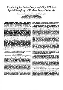
To evaluate the Scopes framework we have conducted numerous experiments on our live testbed. The CS-building building testbed comprises 30 TelosB nodes, powered through USB hubs (see Figure 1), distributed over 9 offices and spanning 544m2 . At each room, nodes are located either next to the windows or above fluorescent lamp tubes. The building’s thick walls greatly reduce radio ranges, forcing a multi-hop behavior even at the maximum transmission power level (0 dBm). Scopes. In our tests we have used the scopes depicted in Figure 1. These represent reasonable, real-life scopes. The scope S1 covers all nodes. Such scopes are necessary, e.g., for massive software updates. Scope S2 emphasizes that membership is not necessarily given by physical proximity, instead scopes build overlays. 2
In this work we investigate the worst case behavior of using only full refreshes, and postpone the analysis of this optimization as a topic for future work.
6
D. Jacobi, P. Guerrero, I. Petrov, and A. Buchmann
Fig. 1: Piloty building testbed and scopes used Finally, S3 and S31 illustrate nested scopes. These occur in any hierarchical relation, for instance, in domain organization. The scope definitions were based on operations on node IDs, although as explained before, other relations over node properties such as location could have been used. Table 2 summarizes the used scopes. The last column presents the size of scope definitions and the entire creation message. These highlight the compactness of the representation. Lastly, all scopes were created at the network boundary, namely node 43 (top left). This forced a minimum of 2 hops and an avgerage of over 3.
Scope Description S1 S2 S3 S31
All nodes Nodes with even id Nodes whose id < 24 || id > 33 Node id ∈ {21, 43, 45, 47, 48}
Parent Scope world world world S3
Scope Def. 4 bytes 74 bytes 9 bytes 24 bytes
Size OS Message 18 bytes 88 bytes 24 bytes 38 bytes
Table 2: Summary of employed scopes
There are two important aspects to the framework, namely reliability and efficiency. In the next subsection we discuss how reliable the scope mechanism is and its relation to the underlying routing protocol. 3.1
Scope Creation, Removal and Maintenance
We first investigate the two main scope operations, creation and removal, together with the scope maintenance. Consider the scope membership described
Distributed Network Structuring with Scopes
7
by a function, φ(t), that outputs the percentage of nodes which belong to a scope out of an expected set at a given time t; φ: Z → [0, 1]. The ideal membership φI (t) is a function of time which equals 100% when the scope is alive and 0% otherwise, that is, resembles an instantaneous scope creation and removal. The values observed in practice, φR (t), lag behind the ideal values, i.e., once a scope is created it takes time for nodes to reach a high membership percentage, and later when a scope is removed it takes time to drop down back to 0%. This is natural and due, e.g., to message propagation delays and medium loss. When multiple test repetitions are considered, we refer to φRmax , φRavg and φRmin as the maximum, average and minimum membership values, respectively. Scope reliability is described by three parameters. First, the reliability level stands for the deviation of the average measured membership percentage values from the ideal ones. To quantify the reliability level, the area between the curves φI and φRavg is calculated. The lower the value is, the closer φRavg is to φI , thus the higher the reliability level. Second, the stability of the scope mechanism indicates its tolerance to network dynamics. This is quantified by calculating the area between the curves φRmax and φRmin . Again, the lower the value, the more stable the membership is. Last but not least, the rapidness in achieving an expected membership percentage is important. We quantify the creation and removal delay by measuring the time it takes for φRavg to arrive to ∼100% after a scope creation, and to 0% after a scope removal, respectively. Clearly, the lower these values, the better. In Figure 2 we characterize the reliability of the framework for S1 and S2 (the behavior of nested scopes is evaluated in detail later) The figures present φRmax , φRavg and φRmin as defined above. A scope is always created at t=0:05 and remains alive for 63 seconds, thus, φI (t) is 100% between t=0:05 and t=1:08, and 0% elsewhere. This scope lifetime allows for 10 refreshes at a period of 6 seconds (indicated with vertical dashed lines drawn at regular intervals). The rightmost dashed vertical line indicates the last point at which all nodes should automatically remove themselves from the scope in case the explicit scope removal message wasn’t heard. This occurs 20 seconds after the last refresh (t=1:25). The plots for S1 , 2(a) and 2(b) show that the creation delay was quite low: it occurred immediately with FLD, while it took 3 refresh periods with GBR. For both algorithms, the scope membership was kept up at around 100% until the explicit removal was requested. Later, once a scope was removed, almost all nodes heard the explicit removal message. Virtually no nodes resorted to the lease expiration timer with FLD (0.26%), while for GBR it was below 5% – an acceptable value. The removal delay of GBR was thus higher than FLD’s (only after the lease expires did nodes automatically release resources). While the reliability levels were similar (FLD got 0.62% while GBR’s was 0.63%), FLD’s stability (2.09%) was better than GBR’s (6.32%). As mentioned before the values for reliability and stability are the deviation to the ideal or min/max curves. The plots for S2 exhibit a slightly lower reliability level. The scope creation delay worsens for FLD, requiring 1 refresh period, and GBR showed an unstable scope
8
D. Jacobi, P. Guerrero, I. Petrov, and A. Buchmann 100
max avg min
100
80
80
70
70
60 50 40 30
60 50 40 30
20
20
10
10
0 00:00 00:10 00:20 00:30 00:40 00:50 01:00 01:10 01:20 01:30 elapsed time [mm:ss]
0 00:00 00:10 00:20 00:30 00:40 00:50 01:00 01:10 01:20 01:30 elapsed time [mm:ss]
(a) FLD, S1 100
(b) GBR, S1 max avg min
90
100
80
80
70
70
60 50 40 30
max avg min
90
scope membership [%]
scope membership [%]
max avg min
90
scope membership [%]
scope membership [%]
90
60 50 40 30
20
20
10
10
0 00:00 00:10 00:20 00:30 00:40 00:50 01:00 01:10 01:20 01:30 elapsed time [mm:ss]
0 00:00 00:10 00:20 00:30 00:40 00:50 01:00 01:10 01:20 01:30 elapsed time [mm:ss]
(c) FLD, S2
(d) GBR, S2
Fig. 2: Scope creation, removal and maintenance for FLD and GBR
membership percentage. The results show that both approaches are viable in practice.
Nested Scopes. We now evaluate the behavior of hierarchical relations among scopes. In these tests, we created scope S3 at t1 , and one second later created subscope S31 . While S3 remained alive (as before) during 63 seconds, S31 remained alive for 33 seconds, which allowed for 5 refreshes to be issued. Figure 3 presents the respective reliability results for FLD and GBR. Again, while both protocols reached high scope membership percentages, GBR (99%) was slightly lower than FLD (100%). The reliability levels were high in both cases: FLD achieved 0.51%, while GBR got 2.95% (lower is better). Also, FLD was more stable than GBR (1.78% vs. 8.89%). The scope creation delay was of 1 refresh period for FLD and 3 for GBR, whereas the removal delay was 20 seconds for FLD and 0 seconds for GBR. These results point out that nested scopes exhibit similar reliability properties to that of top-level scopes.
Distributed Network Structuring with Scopes 100
S3 avg S31 max S31 avg S31 min
90
70 60 50 40 30
S3 avg S31 max S31 avg S31 min
90 80 scope membership [%]
scope membership [%]
80
100
9
70 60 50 40 30
20
20
10
10
0 00:00 00:10 00:20 00:30 00:40 00:50 01:00 01:10 01:20 01:30 elapsed time [mm:ss]
0 00:00 00:10 00:20 00:30 00:40 00:50 01:00 01:10 01:20 01:30 elapsed time [mm:ss]
(a) FLD
(b) GBR
Fig. 3: Scope creation, removal and maintenance for nested scopes S3 and S31
Network Density. We now discuss the effects of network density on scope operations and maintenance. Particularly, we consider the effects of density with respect to the reliability of the scope operations. There are two main effects that influence the reliability. On one side, the more nodes there are, the higher the redundancy available to build the underlying scope overlays, thus the reliability level increases. On the other side, the more nodes there are, the more collisions there can occur, which decreases the reliability level and stability. We inspected this issue by repeating all of our ρ #Nodes Density tests with three node density values. These configu4 30 1/18.1m2 rations are presented in Table 3, with the resulting 2 18 1/30.2m2 density in nodes per m2 . The amount of nodes per 1 10 1/54.4m2 room is indicated with ρ. Figure 4 summarizes the reliability level results Table 3: Node densities for different densities. In general terms, we can say that the denser the network, the higher the reliability level (lower values). Also, and despite the outlier , here it is observed that S1 is more reliable than S2 . Scope Operation Costs. The energy costs associated to the scope operations are largely due to messages sent and received. Evidently, energy efficiency depends on the routing mechanism chosen. We studied the operation cost in isolation, in a typical usage these become marginal compared to data exchange. Figure 5 plots link-level traffic for S1 and S2 . Each measurement point represents one test run (2 minutes), there were 25 runs. The curves confirm the expected routing algorithm behavior. The behavior exhibited by FLD is deterministic, since the decision whether a node is member of a scope or not is totally local: a test run requires around 340 scope management messages regardless of the scope definition. In turn, GBR pays the price of the increased reliability of the acknowledged reverse paths. This overhead, in contrast to flooding, does depend
10
D. Jacobi, P. Guerrero, I. Petrov, and A. Buchmann
on the number of member nodes. Therefore, S1 exhibits a constant factor of 2x, while for S2 it is 1.5x. 3 FLD, S1
GBR, S1
FLD, S2
800
GBR, S2
FLD, S1
GBR, S1
FLD, S2
GBR, S2
700
link-level traffic [m/run]
reliability level [%]
2.5 2 1.5 1
600 500 400 300 200
0.5
100 0 00:00
0 0
1
2
3
network density ρ
4
5
20:00
30:00
40:00
50:00
elapsed time [mm:ss]
Fig. 4: Density tests for S1 and S2
3.2
10:00
Fig. 5: Scope operation costs
Scope Traffic
We proceed by evaluating the bidirectional data channel described in Section 2.1. As important metrics, we consider goodput and link level message exchange. While the former refers to the end-to-end application layer traffic, the latter indicates the in-network traffic needed to obtain that goodput. We have designed our traffic tests as illustrated in Figure 6. During the first [t0 , t1 ) and last (t4 , t5 ] stages, there’s no activity. A scope is created at t1 , and remains alive until it is removed at t4 . In order to allow the scope to stabilize after its creation and removal, we introduce an initial delay of α and a wait of β seconds (respectively). Traffic itself occurs during (t2 , t3 ). The two traffic directions, root-to-members (RtM) and members-to-root (MtR), were tested separately. For theroot-to-members RtM tests we chose α=15s and β=3s. This large or members-to-root 25 sec. a delay b wait scoped data traffic auto-scope removal α value allows the scope to stabilize through two refreshes before data transscope alive mission starts. For the MtR tests we chose α=3s and β=20s. Here, a short α no scope was sufficient, tbut a larger (i.e., t2 β was needed to accountt3 for removed t4 t5 unsta0 t1 ble) nodes. More importantly, since sensor network applications are diverse, we concentrate on two communication patterns: periodic and bursty traffic. POST timer, [2 s]
t
Mx
SEND timer [0.25s + e], 0s< e