Distributed PCA and Network Anomaly Detection - BNRG - UC Berkeley

Distributed PCA and Network Anomaly Detection

Ling Huang Xuanlong Nguyen Minos Garofalakis Michael Jordan Anthony D. Joseph Nina Taft

Electrical Engineering and Computer Sciences University of California at Berkeley Technical Report No. UCB/EECS-2006-99 http://www.eecs.berkeley.edu/Pubs/TechRpts/2006/EECS-2006-99.html

July 14, 2006

Copyright © 2006, by the author(s). All rights reserved. Permission to make digital or hard copies of all or part of this work for personal or classroom use is granted without fee provided that copies are not made or distributed for profit or commercial advantage and that copies bear this notice and the full citation on the first page. To copy otherwise, to republish, to post on servers or to redistribute to lists, requires prior specific permission.

Distributed PCA and Network Anomaly Detection Ling Huang∗

XuanLong Nguyen∗

Michael Jordan∗ ∗

UC Berkeley

Minos Garofalakis†

Anthony Joseph∗ †

Nina Taft†

Intel Research Berkeley

{hling, xuanlong, adj, jordan}@cs.berkeley.edu

{minos.garofalakis, nina.taft}@intel.com

Abstract We consider the problem of network anomaly detection given the data collected and processed over large distributed systems. Our algorithmic framework can be seen as an approximate, distributed version of the well-known Principal Component Analysis (PCA) method, which is concerned with continuously tracking the behavior of the data projected onto the residual subspace of the principal components within error bound guarantees. Our approach consists of a protocol for local processing at individual monitoring devices, and global decision-making and monitoring feedback at a coordinator. A key ingredient of our framework is an analytical method based on stochastic matrix perturbation theory for balancing the tradeoff between the accuracy of our approximate network anomaly detection, and the amount of data communication over the network.

1 Introduction The area of distributed computing systems provides a promising domain for applications of machine learning methods. One of the most interesting aspects of such applications is that learning algorithms that are embedded in a distributed computing infrastructure are themselves part of that infrastructure and must respect its inherent local computing constraints (e.g., constraints on bandwidth, latency, reliability, etc.), while attempting to aggregate information across the infrastructure so as to improve system performance (or, availability) in a global sense. Consider, for example, the problem detecting anomalies in a wide-area network. While it is straightforward to embed learning algorithms at local nodes to attempt to detect node-level anomalies, these anomalies may not be indicative of network-level problems. Indeed, in recent work, [10] demonstrated a useful role for Principal Component Analysis (PCA) to detect network anomalies. They showed that the minor components of PCA (the subspace obtained after removing the components with largest eigenvalues) revealed anomalies that were not detectable in any single node-level trace. While their work did not face the distributed data analysis problem (it involved centralized, off-line analysis of blocks of data), it does provide clear motivation for attempting to design a distributed PCA-based system for analyzing network anomalies in real time. The development of such a design involves facing several challenging problems that have not been addressed in previous work. Naive solutions that continuously push all data to a central analysis site simply cannot scale to large networks or massive data streams. Instead, viable solutions need to process data “in-network” to intelligently control the frequency and size of data communications. The key underlying problem is that of developing a mathematical understanding of how to trade off quantization arising from local bandwidth restrictions against fidelity of the data analysis. We also need to understand how this tradeoff impacts overall detection accuracy. Finally, the implementation needs to be simple if it is to have impact on developers. In this paper, we present a simple algorithmic framework for approximate distributed PCA tracking, together with supporting theoretical analysis. In brief, the architecture involves a set of local monitors that maintain parameterized sliding filters. These sliding filters yield quantized data streams

that are sent to a coordinator. The coordinator makes global decisions based on these quantized data streams, and also provides feedback to the monitors, allowing them to update the parameters of their filters. Our basic theoretical tool is stochastic matrix perturbation theory. This tool turns out to be quite well suited to our problem, yielding analytical expressions or explicit bounds for many of the quantities that are needed in either our approximate PCA-tracking algorithm or in the analysis of its performance guarantees. The combination of our theoretical tools and local filtering strategies results in a distributed tracking algorithm that can achieve high detection accuracy with low communication overhead; for instance, our experiments show that, by choosing a relative eigen-error of 1.5% (yielding, approximately, a 4% missed detection rate and a 6% false alarm rate), we can filter out more than 90% of the traffic for the original signal. Prior Work. The original work on PCA-based methods by Lakhina et al. [10] has been extended by [20], who show how to infer network anomalies in both spatial and temporal domains. As with [10], this work is completely centralized. Other initiatives in distributed monitoring, profiling and anomaly detection aims to share information and foster collaboration between widely distributed monitoring boxes to offer improvements over isolated systems [13, 18, 19]. In the setting of simpler statistics such as sums and counts, distributed detection methods related to ours have been explored by [8]. Finally, work in the machine learning literature that combines learning methods with distributed constraints includes work by [12], who introduce a distributed kernel-based classification algorithm and [9], who consider a distributed message passing algorithm in graphical models. Organization. We start by discussing our system model and background on PCA-based network traffic anomaly detection in Section 2. Section 3 presents our distributed PCA-tracking algorithm and highlights our main analytical results. (Due to space constraints, detailed proof arguments can be found in the appendix.) We present the experimental evaluation of our system in Section 4, and give our conclusions in Section 5.

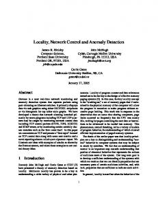
2 Problem description and background We consider a monitoring system comprising a set of local monitor nodes M 1 , . . . , Mn each of which collects a locally-observed time-series data stream (Fig. 1(a)). For instance, the monitors may collect information on the number of TCP connection requests per second, the number of DNS transactions per minute, or the volume of traffic at port 80 per second. A central coordinator node aims to continuously monitor the global collection of time series, and make global decisions such as those concerning matters of network-wide health. Although our methodology is generally applicable, in this paper, we focus on the particular application of detecting volume anomalies. A volume anomaly refers to unusual traffic load levels in a network that are caused by anomalies such as worms, DDoS attacks, device failures, misconfigurations, and so on. Each monitor collects a new data point at every time step and, assuming a naive, “continuous push” protocol, sends the new point to the coordinator. Based on these updates, the coordinator keeps track of a sliding time window of size m (i.e., the m most recent data points) for each monitor time series, organized into a matrix Y of size m × n (where the ith column Yi captures the data from monitor i, see Fig. 1(a)). The coordinator then makes its decisions based solely on this (global) Y matrix. The network-wide volume anomaly detection algorithm of [10] works by local monitors measuring the total volume of traffic (in bytes) on each network link, and periodically (e.g., every 5 minutes) centralizing the data by pushing all recent measurements to the coordinator. The coordinator then performs PCA on the assembled Y matrix to detect volume anomalies. (Details are given later in this section.) This method has been shown to work remarkably well, in part due to the inherently low-dimensional nature of the underlying data. However, such a “periodic push” approach suffers from inherent limitations: To ensure fast detection, the update periods should be relatively small; unfortunately, small periods also imply increased monitoring communication overheads, which may very well be unnecessary (e.g., if there are no significant local changes across periods). Instead, in our work, we study how the monitors can effectively filter their time-series updates, sending as little as possible, yet enough so as to allow the coordinator to make global decisions accurately. We provide analytical bounds on the errors that occur because decisions are made with incomplete data, and explore the tradeoff between reducing data transmissions (communication overhead) and decision accuracy.

18

3

Anomaly

x 10

Data Flow

ˆ = Y

State Vector

Result

2

1

0

Mon

Tue

Wed

Thu

Fri

Sat

Sun

Tue

Wed

Thu

Fri

Sat

Sun

17

Y=

M1

M2

1

M3

Mn

4

3

2

3

7

6

5

5

2

1

8

Residual Vector

2

x 10

1.5 1 0.5 0

Mon

(a) The system setup

(b) Abilene network traffic data

Figure 1: (a) The distributed monitoring system; (b) Data sample (kyk2 ) collected over one week (top); its projection in residual subspace (bottom). Dashed line represens a threshold for anomaly detection.

Using PCA for centralized volume anomaly detection. As observed by Lakhina et al. [10], due to the high level of traffic aggregation on ISP backbone links, volume anomalies can often go unnoticed by being “buried” within normal traffic patterns (e.g., the circle dots shown in the top plot in Fig 1(b)). On the other hand, they observe that, although, the measured data is of seemingly high dimensionality (n = number of links), normal traffic patterns actually lie in a very low-dimensional subspace; furthermore, separating out this normal traffic subspace using PCA (to find the principal traffic components) makes it much easier to identify volume anomalies in the remaining subspace (bottom plot of Fig. 1(b)). As before, let Y be the global m × n time-series data matrix, centered to have zero mean, and let y = y(t) denote a n-dimensional vector of measurements (for all links) from a single time step t. Formally, PCA is a coordinate-transformation method that maps a given set of data points onto principal components ordered by the amount of data variance that they capture. The set of n principal components, {vi }ni=1 , are defined as: i−1 X vi = arg max k(Y − Yvj vjT )xk kxk=1

j=1

and are the n eigenvectors of the estimated covariance matrix A := Y T Y. As shown in [10], PCA reveals that the Origin-Destination (OD) flow matrices of ISP backbones have low intrinsic dimensionality: For the Abilene network with 41 links, most data variance can be captured by the first k = 4 principal components. Thus, the underlying normal OD flows effectively reside in a (low) k-dimensional subspace of Rn . This subspace is referred to as the normal traffic subspace Sno . The remaining (n − k) principal components constitute the abnormal traffic subspace S ab .

Detecting volume anomalies relies on the decomposition of link traffic y = y(t) at any time step into normal and abnormal components, y = yno +yab , such that (a) yno corresponds to modeled normal traffic (the projection of y onto Sno ), and (b) yab corresponds to residual traffic (the projection of y onto Sab ). Mathematically, yno (t) and yab (t) can be computed as yno (t) = PPT y = Cno y and yab (t) = (I − PPT )y = Cab y where P = [v1 , v2 , . . . , vk ], is formed by the first k principal components which capture the dominant variance in the data. The matrix Cno = PPT represents the linear operator that performs projection onto the normal subspace Sno , and, Cab projects onto the abnormal subspace Sab .

As observed in [10], a volume anomaly typically results in a large change to y ab ; thus, a useful metric for detecting abnormal traffic patterns is the squared prediction error (SPE): SPE ≡ kyab k2 = kCab yk2

Distr. Monitors ?

δ1 - Filter/ Predict

-

Anomaly

?

R1 (t) Coordinator

Y2(t)

?

δ2 - Filter/ Predict

6



Y1(t)

Residual Thresholding 

R2 (t)

^ q

Perturbation Analysis

-

6

−error PCA

Low-Rank Update

 ~

Yn (t)

?

δn- Filter/ Predict

Rn (t)

?

Adaptive Slacks

Figure 2: Our distributed tracking and detection framework. (essentially, a quadratic residual function). More formally, their proposed algorithm signals a volume anomaly, if SPE > Qα , where Qα denotes the threshold statistic for the SPE residual function at the 1 − α confidence level. Such a statistical test for the SPE residual function, known as the Qstatistic [7], can be computed as a function Qα = Qα (λk+1 , . . . , λn ), of the (n − k) non-principal eigenvalues of the covariance matrix A.

3 Distributed PCA for anomaly detection We now describe our communication-efficient distributed solution for real-time approximate PCA tracking and detection. In a nutshell, the key idea is to limit monitor-coordinator interactions by installing local filters at the monitors, and forcing communication only when such local constraints are violated. Using stochastic matrix perturbation theory to analyze the effect of this local quantization on the global matrix PCA, we propose a simple, adaptive distributed protocol with useful, provable performance guarantees on the communication/detection accuracy tradeoff. 3.1 Overview of our approach Our approach for distributed, PCA-based anomaly detection comprises two parts: (1) the monitors process their collected data by applying local filtering rules to suppress unnecessary message updates to the coordinator; and, (2) the coordinator makes global detection decisions and provides feedback to the monitors (e.g., local filter parameter settings) based on the observed updates. Fig. 2 illustrates the overall architecture of our distributed anomaly-detection system. Local Processing at Monitors. The goal of a monitor is to track its local raw data stream, and update the coordinator of any considerable drift that might affect the global decision made by the coordinator. Of course, our goal is to avoid flooding the coordinator with all the raw data. To this end, each monitor i maintains a filtering window Fi (t) of size 2δi centered at a value Ri (i.e., Fi (t) = [Ri (t) − δi , Ri (t) + δi ]). The monitor updates the coordinator with the most recent data Yi (t) only if Yi (t) ∈ / Fi (and sends nothing otherwise).

The window parameter δi is called the slack. Clearly, increased slack implies reduced communication between a monitor and the coordinator at the expense of potential information loss (i.e., poor approximation) at the the coordinator. The center parameter R i (t) denotes the approximate representation of Yi (t) that the coordinator uses; in general, Ri (t) can be based on any type of filtering/prediction model for node Mi ’s behavior over time. (For instance, in our implementation, Ri (t) is simply the average of last five signal values observed locally at monitor i.) Obviously, this ˆ of the Y matrix. implies that the coordinator maintains only an approximate “filtered” version Y Global Decision-Making at the Coordinator. The role of the coordinator is twofold. First, it makes global anomaly-detection decisions based upon the received updates from monitors. Secondly, it provides feedback to the monitors in order to adjust their filtering windows’ slack and

center parameters. The global detection task is the same as the centralized detection scheme deˆ on the scribed in Section 2 using the SPE statistic based on the projection of a filtered signal y residual subspace represented by matrix Sab . In contrast to the centralized setting, however, the coordinator does not have an exact version of the raw data matrix Y; instead, PCA is performed and ˆ := A − ∆, where the Sab is computed on the perturbed/filtered version of the covariance matrix A magnitude of the perturbation matrix ∆ is decided by the slack variables δ i (i = 1, . . . , M ). 3.2 Distributed tracking of eigenvalues and the residual subspace A key ingredient of our framework is a practical method for choosing slack parameters δ i that effectively balance the tradeoff between the desirable loss of detection accuracy (i.e., due to the use ˆ instead of Y) and the savings in data communication. The mathematical tool that we employ of Y to resolve this issue is stochastic matrix perturbation theory. This theory quantifies the effects of the perturbation of a matrix on key quantities such as eigenvalues and the eigen-subspaces, which in turn affects the detection accuracy. In the remainder of this section, we highlight several key results of our analysis; due to space constraints, the complete details can be found in the appendix. ˆ = Y + W, In our framework, the coordinator’s view of the data matrix is the perturbed matrix Y where all elements of the column vector Wi are bounded within interval [−δi , δi ]. Let λi and ˆ i (i = 1, . . . , n) denote the eigenvalues of the covariance matrix A = Y T Y and its perturbed λ ˆ T Y. ˆ Applying classical theorems of Mirsky and Weyl [17], we obtain bounds ˆ := Y version A on the eigenvalue perturbation in terms of the Frobenius norm k.k F and the spectral norm k.k2 of ˆ respectively: ∆ := A − A, v u n uX 1 √ ˆ i − λi | ≤ k∆k2 ˆ i − λi )2 ≤ k∆kF / n and max|λ eig := t (1) (λ i n i=1 Applying the sin theorem and results on bounding the angle of projections to subspaces [3, 17] (see the appendix for more details), we also obtain bounds on the perturbation of the residual subspace Cab in terms the Frobenius norm of ∆: √ 2k∆kF ˆ kCab − Cab kF ≤ (2) ν

where ν denotes the eigengap between the k th and (k +1)th eigenvalues of the estimated covariance ˆ matrix A. The issue is to obtain practically useful bound on the norms of ∆. To this end, we obtain expectation bounds instead of worst case bounds. We make the following assumptions on the error matrix W: 1. The column vectors W1 , . . . , Wn are independent and radially symmetric m-dim vectors. 2. For each i = 1, . . . , n, all elements of column vector Wi are i.i.d. random variables with mean 0, variance σi2 := σi2 (δi ) and fourth moment µ4i := µ4i (δi ). Note that the independence assumption is on the error only – this by no means implies that the signals received by different monitors are statistically independent. We define the aggregated variance P √ 2 across monitors as σ := n i=1 σi . Under the above assumption, we can show that k∆k F / n is upper bounded by the following quantity with high probability when m and n are large: v v u n u n n uσ X u 2X mX 4 m ˆi + t m T olF = 2t σi4 + (µ − σi4 ) + σ 2 λ (3) n i=1 n i=1 n i=1 i n Similar results can be obtained for the spectral norm as well. In practice, these upper bounds are very tight because σ tends to be small compared to the top eigenvalues.

In summary, given the tolerable perturbation T olF on the norm of the covariance matrix, we can decide the amount of slack for each monitor via Equation. (3) (e.g., by dividing the overall tolerance across monitors either uniformly or in proportion to their observed local variance). At the same time, the bounds (1) and (2) allow us to measure the amount of perturbation  eig in terms of eigenvalues, which affects the detection accuracy, which we discuss next.

3.3 Effects on detection procedure at the coordinator ˆ We now address The coordinator performs online detection based upon the (filtered) data stream Y. the impact of approximation in PCA on the detection procedure. Specifically, we examine how the filtering on Y impacts the residual projection statistic SPE = kCab yk2 and the threshold Qα . As discussed, using filtering slacks computed by Equation 3, the coordinator can bound the deviation ˆ α from their true values, which gives us tools to analyze and bound ˆ ab k and Q of its computed kC ˆ α . First, ˆ ab y ˆ k2 > Q the false alarm rate on the detection at the coordinator when using condition k C note that √ n X 2k∆kF kˆ yk ˆ ˆ ˆ k − kCab yk| ≤ k(Cab − Cab )ˆ ˆ )k ≤ δi2 |kCab y yk + kCab (y − y + kCab k2 ν i=1 ! n √ √ X 2k∆kF kˆ yk ˆ ab k + 2k∆kF δi2 =: η1 (ˆ y) ≤ + kC ν ν i=1 It is simple to obtain an upper bound on the perturbation of SPE as: ˆ ab y ˆ k + η1 (ˆ η2 (ˆ y) = η1 (ˆ y)(2kC y)). Turning to the threshold Qα , which is given as a function of λk+1 , . . . , λn , the eigenvalues of A [7]: " p # h1 cα 2φ2 h20 φ2 h0 (h0 − 1) 0 Qα = φ1 +1+ φ1 φ21 where cα is the (1 − α)-percentile of the standard normal distribution, h0 = 1 − 2φ3φ1 φ2 3 , φi = 2 Pn i j=k+1 λj for i = 1, 2, 3. The perturbation in λk+1 , . . . , λn directly impacts the change of Qα . In our application, it is observed that the change of φ1 usually dominates the change. Furthermore, increasing φ1 results in decreasing Qα . Since the addition of random perturbation to a matrix tends to increase the non-principal eigenvalues λk+1 , . . . , λn , thus increasing φ1 . This implies that Qα decreases as the amount of perturbation increases. To assess the perturbation in terms of false alarm rate, we only need to bound the difference cˆ − c, where cˆ is a perturbed version of: c=

φ1 [(SPE/φ1 )h0 − 1 − φ2 h0 (h0 − 1)/φ21 ] p . 2φ2 h20

Let ηc denote the bound on |ˆ c −c|. The change to the false alarm rate is approximated as P (c α −ηc < U < cα + ηc ), where U is a standard normal random variable.

4 Evaluation We implemented our algorithm and developed a trace-driven simulator to validate our methods. We used a one-week trace collected from the the Abilene network1. The traces containes per-link traffic loads measured every 10 minutes, for all 41 links of the Abilene network. With a time unit of 10 minutes, data was collected for 1008 time units. This data was used to feed in the simulator. There are 7 anomalies in the data that were detected by the centralized algorithm (and verified by hand to be true anomalies). In our experiments, we injected 70 synthetic anomalies into this dataset using the method described in [10], so that we would have sufficient data to compute error rates. We used a threshold Qα corresponding to an 1 − α = 99.5% confidence level. Due to space limitations, we only present results for the case of uniform monitor slack δi = δ. The input parameter for algorithm is the tolerable relative error of eigenvalues (relative eigen error in short), which acts as a tuning knob.2 Given this parameter and the input data we can compute 1 Abilene is an Internet2 high-performance backbone network that interconnects a large number of universities as well as a few other q research institutes. P 2 2 λi , where T olF is defined in Eqn (3). Precisely, it is T olF / n1

the filtering slack δ for the monitors using Eqn (3). We then feed in the data to run our protocol in the simulator with the computed δ. The simulator outputs a set of results including: 1) the actual relative eigen errors and the relative errors on the detection threshold Q α ; 2) the missed detection rate, false alarm rate and communication cost when using our protocol for distributed tracking and anomaly detection. The missed-detection rate is defined as the fraction of missed detections over the total number of real anomalies, and the false-alarm rate as the fraction of false alarms over the total number of detected anomalies by our protocol. The communication cost is computed as the fraction of number of messages that actually get through the filtering window to the coordinator. The results are shown in Fig. 3. In all plots, x-axis is the tolerable relative eigen error. In Fig. 3(a) we plot the relationship between the tolerable eigen error and filtering slack δ when assuming filtering errors are uniformly distributed on interval [−δ, δ]. With this model, the relationship between the tolerable eigen error and the slack is determined by a simplified version of Eqn (3). The results make intuitive sense. As we increase our error tolerance, we can filter more at the monitor and send less to the coordinator. The slack increases almost linearly with the tolerable eigen error because the first term in the right hand side of Eqn (3) dominates all other terms. In Fig. 3(b) we compare the tolerable relative eigen error (which is the tuning parameter) to the q P 1 λ2i , where eig is defined in actual accrued relative eigen error (precisely defined as eig / n Eqn (1)). These were computed using the slack parameters δ as computed by our coordinator. We can see that the real accrued eigen errors are always less than the tolerable eigen errors. The plot shows a tight upper bound, indicating that it is safe to use our model’s derived filtering slack δ. In other words, the achieved eigen error always remains below the requested tolerable error specified as input, and the slack chosen given the tolerable error is close to being optimal. In Fig. 3(c) we show the relationship between the tolerable eigen error and the relative error of detection threshold Qα 3 . It confirmed our analysis that the threshold for detecting anomalies decreases as we tolerate more and more eigen errors. In these experiments, an error of 2% in the eigenvalues, leads to an error of approximately 6% in our estimate of the appropriate cutoff threshold. We are now ready to examine the false alarm rates achieved. In Fig. 3(d) the curve with triangles represents the upper bound on the false alarm rate as estimated by the coordinator (as discussed in section 3.3). The curve with circles is the actual accrued false alarm rate achieved by our scheme. It is worth noting that the upper bound on the false alarm rate is fairly close to true values, especially when the slack is small. The false alarm rate increases with increasing eigen error because as the eigen error increases, the corresponding detection threshold Q α will decrease, which in turn causes ˆ rather than the relative threshold the protocol to raise an alarm more often. (If we had plotted Q ˆ difference, we would obviously see a decreasing Q with increasing eigen error.) To the best of our knowledge, this is among the first work to provide a bound on false alarm rates for a network anomaly detector in a distributed setting. In Fig. 3(e) we present the missed detection rates. For varying choice of communication overhead the missed detection rate remains below 4%. Finally we examine the communication overhead in Fig. 3(f). As we can tolerate larger errors, we can consequently reduce the overhead. Using these last three plots (d,e,f) together, we can observe the tradeoffs that occur. For example, when the relative eigen error is 1.5%, our algorithm reduces the data sent through the network by more than 90%. This gain is achieved at the cost of approximately a 4% missed detection rate and a 6% false alarm rate. This is a large reduction in communication for a small increase in detection errors. This illustrates that our distributed protocol can achieve high detection accuracy with low communication overhead.

5 Conclusion We have presented a distributed algorithmic framework for network anomaly detection using the PCA method. Our framework consists of a simple protocol for local data processing at the monitoring devices and global decision making and feedback at the coordinator. Using tools for stochastic matrix perturbation theory, we provided an analysis for the tradeoff between the detection accuracy 3

ˆ k+1 , . . . , λ ˆn . ˆ α /Qα , where Q ˆ α is computed from λ Precisely, it is 1 − Q

7

Fal. Alarm Rate

2

0

0.005

0.01

0.015

0.015

(a)

0.02

0.025

0.03

0.01

Rel. Threshold Error

0.005 0

0

0.005

0.01

0.1

0.015

(b)

0.02

0.025

0.03

0.05

0

0

0.005

0.01

0.015

(c)

0.02

0.025

0.03

Missed Detec. Rate

4

0 Rel. Eigen Error

x 10

0.4

Upper Bound Actual Accrued

0.3 0.2 0.1 0

0

0.005

0.01

0.015

0.02

0.025

0.03

0

0.005

0.01

0.015

0.02

0.025

0.03

0

0.005

0.01

0.015

0.02

0.025

0.03

0.1

(d)

0.05

Comm. Overhead

Slack

6

0 1

(e)

0.5

0

(f)

Figure 3: Parameters design, communication overhead and accrued error. and the data communication overhead. In particular, using relative eigen error as a tuning knob, we were able to control the amount of data overhead, and as well as provide upper bounds on the false alarm rate. Our algorithm is simple to implement, and is empirically shown to yield high accuracy of anomaly detection in Abilene network despite using very little data.

References [1] A LON . N., K RIVELEVICH , M., AND V U , V. H. On the concentration of eigenvalues of random symmetric matrices. In Israel J. Math, 131 (2002), pp. 259-267. [2] B OTTCHER , A. AND G RUDSKY, S. The norm of the product of a large matrix and a random vector. In Electronic Journal of Probability, Vol. 8 (2003), pages 1-29. [3] DRMAC, Z. On principal angles between subspaces of euclidean of space In SIAM J. Matrix Anal. Appl., 22(1) 2000. [4] G EMAN , S. A limit theorem for the norm of random matrices. In Ann. Probab., 8 (1980), pp. 252-261. [5] H OLMES , R. B. On Random Correlation Matrices. IN SIAM J. Matrix Anal. Appl., 12(2) 1991. [6] H UANG , L., G AROFALAKIS , M., J OSEPH , A. AND TAFT, N. Communication-efficient tracking of distributed cumulative triggers. Under submission, May 2006. [7] JACKSON , J. E. AND M UDHOLKAR , G. S. Control procedures for residuals associated with principal component analysis. In Technometrics, pages 341-349, 1979. [8] K ERALAPURA , R., C ORMODE , G. AND R AMAMIRTHAM , J. Communication-efficient distributed monitoring of thresholded counts To appear in ACM SIGMOD (2006). [9] K REIDL , P. O., W ILLSKY, A. Inference with Minimal Communication: a Decision-Theoretic Variational Approach. In NIPS 18 (2006). [10] L AKHINA , A., C ROVELLA , M. AND D IOT, C. Diagnosing network-wide traffic anomalies. In ACM SIGCOMM, (2005). [11] L AKHINA , A., PAPAGIANNAKI , K., C ROVELLA , M., D IOT, C., KOLACZYK , E. D. AND TAFT, N. Structural analysis of network traffic flows. In ACM SIGMETRICS, (2004). [12] N GUYEN , X., WAINWRIGHT, M. AND J ORDAN , I. M. Nonparametric decentralized detection using kernel methods. In IEEE Trans. Signal Processing 53(11), (2005). [13] PADMANABHAN , V. N., R AMABHADRAN , S., AND PADHYE , J. Netprofiler: Profiling wide-area networks using peer cooperation. In IPTPS (2005).

[14] RUBINSTEIN , R. Generating random vectors uniformly distributed inside and on the surface of different regions. In Europ. J. Oper. Res., 10 (1982), pp. 205-209. [15] S PRING , N., W ETHERALL , D., AND A NDERSON , T. Scriptroute: A facility for distributed internet measurement. In USITS (2003). [16] S TEWART, G. W. Perturbation theory for the sigular value decomposition. UMIACS-TR-90-123, 1990. [17] S TEWART, G. W., AND S UN , J.-G. Matrix Perturbation Theory. Academic Press, 1990. [18] X IE , Y., K IM , H.-A., O’H ALLARON , D. R., R EITER , M. K., AND Z HANG , H. Seurat: A pointillist approach to anomaly detection. In RAID (2004). [19] Y EGNESWARAN , V., BARFORD , P., AND J HA , S. Global intrusion detection in the domino overlay system. In NDSS (2004). [20] Z HANG , Y., G E , Z.-H., G REENBERG , A., AND ROUGHAN , M. Network anomography. In IMC , (2005).

6 Appendix In this Appendix we develop a more detailed analysis of the impact of the slackness parameter (δ1 , . . . , δn ) on the eigenvalues and eigen subspaces on the principal components using matrix perturbation theory. Some of the main results presented herein are summarized in Section 3. We begin with a brief background description of known results from matrix perturbation theory, and then proceeds to its application on our problem. 6.1 Background Matrix perturbation theory is concerned with measuring the impact of small perturbation on matrices on relevant quantities such as the eigenvalues and eigenvectors. Eigenvalue perturbation bounds The basic perturbation bounds for eigenvalues of a matrix are due to Weyl and Mirsky with following two theorems [16]. Let matrix A has eigenvalues λ i , and its ˆi , for i = 1, . . . , n. We have: ˆ = A + ∆, has eigenvalues λ perturbated matrix, A Theorem 1 (Weyl) Theorem 2 (Mirsky)

ˆ i − λi | ≤ k∆k2 . maxi |λ q P n 1 n

ˆ − λ i )2 ≤

i=1 (λi

k∆kF √ n

.

Here k.k2 and k.kF denote the spectral 2-norm and the Frobenius norm (cf. [17]). Invariant subspace perturbation. While eigenvalues are quite stable under matrix perturbation, the individual eigenvectors are not. Instead one needs to look at the perturbation of subspaces spanned by the eigenvectors. Subspaces spanned by eigenvectors are an example of invariant subspaces, which are known to be stable 4 Let L(·) denote the set of eigenvalues of a matrix, S(·) denote the subspace spanned by a matrix, and Θ denote the matrix of canonical angle between two subspaces (cf. [17]). Then the perturbation of an invariant subspace spanned by eigenvectors can be quantify by the sin of the canonical angle by the following sin Θ theorem [17]: Theorem 3 Let A have the spectral resolution  T   X1 L1 X X ] = A [ 1 2 0 XT 2

0 L2



where [ X1 X2 ] is unitary with X1 ∈ Cn×k . Let Z ∈ Cn×k have orthonormal columns, and for any symmetric M of order k, let R = AZ − ZM

suppose that L(M) ⊂ [a, b] and for some eigengap ν > 0,

L(L2 ) ⊂ R\[a − ν, b + ν] 4

A subspace X is invariant of transformation A if AX ⊂ X .

Then for any unitarily invariant norm k sin Θ [S(X1 ), S(Z)] k ≤

kRk ν

Note that this theorem applies to any unitarily invariant norm such as the spectral norm k.k 2 and Frobenius norm k.kF . Applying this result to the eigen subspaces for (symmetric) covariance matrix ˆ assume that A ˆ has the following the spectral resolution A and its purturbed version A,    T  M1 0 Z1 ˆ A [ Z1 Z2 ] = 0 M2 ZT 2 ˆ 1 = M1 and AZ ˆ 1 = where [ Z1 Z2 ] is unitary with Z1 ∈ Cn×k . Then we have Z1 T AZ ˆ Z1 M1 . Let R = AZ1 − Z1 M1 = AZ1 − AZ1 = ∆Z1 . For any unitarily invariant norm, there holds kRk = k∆Z1 k = k∆k. As a result, we have: kRk k∆k = ν ν Finally, there is a close relationship between the perturbation of the projection operator onto invariant subspaces and the canonical angle of the subspace perturbation. Let P X and PZ be the orthogonal projections onto S(X) and S(Z). There holds [17]: k sin Θ [S(X1 ), S(Z1 )] k ≤

kPX − PZ kF

=

√

2k sin Θ [S(X), S(Z)] kF ≤

k∆kF . ν

In summary, in order to assess the perturbation in eigenvalues and eigensubspace, we need to estimate the upper bounds given in terms of the Frobenius norm and the spectral norm of ∆. 6.2 Error matrix analysis For the remainder of this appendix we shall present bounds and estimation of the Frobenius norm ˆ T Y, ˆ where Y ˆ = Y + W. ˆ =Y and spectral norm of the perturbation. Recall that A = Y T Y and A Wi is a column vector of filtering error at each monitor i and W is the filtering (perturbation) error on the distributed matrix Y. Each element eji of vector Wi is assumed to be bounded within ˆ can be bounded as follows: [−δi , δi ]. The norm of the perturbation error matrix ∆ = A − A k∆k = kYT W + WT Y + WT Wk ≤ kYT Wk + kWT Yk + kWT Wk.

Our strategy is to obtain bounds for each terms in the RHS of this inequality. It is possible to derive absolute bounds in terms of the absolute error δi (i = 1, . . . , n). However, such bounds would be too loose for practical purposes. Instead, we appeal to stochastic perturbation theory. The basic idea is to assume that the error matrix W is random according to a certain distribution with estimated mean and higher-order moments. Instead of estimating the absolute upper bound for k∆k, we focus on estimating or bounding Ek∆k. This is done by bounding the expectation of the terms on the RHS of the above inequality. Our assumption on the random distribution of W is given as follows: 1. The column vectors W1 , . . . , Wn are independent and radially symmetric m-dim vectors. 2. For each i = 1, . . . , n, all elements of column vector Wi are i.i.d. random variables with mean 0, variance σi2 := σi2 (δi ) and fourth moment µ4i := µ4i (δi ). 6.2.1 Analysis of Frobenius norm Computation of EkY T Wk2F . We exploit results from [2]: For any m-dimensional random vector v uniformly distributed on the unit sphere Sm−1 , and given a m × n matrix Y, there hold: E(kYT vk2 ) =

kYT k2F , m

Var(kYT vk2 ) ≤

2 m+2

As observed in [14], since Wi is assumed to be radially symmetric m-dimensional random vector, its projection on the unit sphere as Wi = vi · kWi k, where vi is uniformly distributed on Sm−1 , and is independent with kWi k. Then we have E(kYT Wi k2 ) = E(kYT vi k2 · kWi k2 ) = E(kYT vi k2 ) · E(kWi k2 ) E(kWi k2 ) = kYk2F · σi2 = kYk2F · m n n X X E(kYT Wi k2F ) kYT Wi k2F ) = E(kYT Wk2F ) = E(kYT Wk2F ) = E( i=1

i=1

=

n X i=1

kYk2F · σi2 = kYk2F ·

= tr(YT Y) ·

n X

σi2 =

i=1

n X i=1

n X

σi2

i=1

λi ·

n X

n X

σi2 =

i=1

i=1

λi · σ,

where λ0i s are eigenvalues of covariance matrix A = Y T Y.5 Computation of E(kWT Wk2F ) This is a high order term, and its value is generally dominated by EkYT Wk2F . Our computation relies on the assumption that the error vectors W 1 , . . . , Wn are independent. In addition, we use the following fact from [5]: if u, v are independently and uniformly distributed column vectors on Sm−1 , then there hold: E(uT · v) = 0,

E[(uT · v)2 ] =

1 , m

Var[(uT · v)2 ] =

2(m − 1) m2 (m + 2)

For i 6= j, we have E[(WiT Wj )2 ]

= E

"

WiT Wj · kWi k kWj k

2

2

· kWi k · kWj k

2

#

=

1 · E(kWi k2 · kWj k2 ) m

m2 σi2 σj2 1 · E(kWi k2 ) · E(kWj k2 ) = = mσi2 σj2 m m P 2 Define zi := WiT Wi = m j=1 eji . We have =

E(e2ji ) = σi2 ,

Var(e2ji ) = E(e4ji ) − (E(e2ji ))2 = µ4i − σi4

Then we have E(zi ) = E(

m X

e2ji ) =

j=1 m X

Var(zi ) = Var(

j=1

m X

E(e2ji ) = mσi2

j=1 m X

e2ji ) =

j=1

Var(e2ji ) = m(µ4i − σi4 )

E(zi2 ) = (E(zi ))2 + Var(z) = m2 σi4 + m(µ4i − σi4 ) In sum, we have E(kWT Wk2F )

=

n X

E[(WiT Wi )2 ] + 2

i=1

= m2

E[(WiT Wj )2 ]

i=1 j=i+1

n X i=1

5

n n X X

σi4 + m

n X i=1

(µ4i − σi4 ) + 2

n n X X

mσi2 σj2

i=1 j=i+1

For simplicity, we typically suppress the dependence on δ in our notations, such as using σ instead of σ(δ).

p Expectation bounds An application of Jensen’s inequality yields E(x) ≤ E(x2 ). Then we can upper bound E(k∆kF ) as follows q q E(k∆kF ) ≤ 2E(kYT WkF ) + E(kWT WkF ) ≤ 2 E(kYT Wk2F ) + E(kWT Wk2F ) v v u n u X n n n n n X X X X uX u 2 4 4 4 2 t t λi · σi + m σi + m (µi − σi ) + 2 mσi2 σj2 = 2 i=1

i=1

i=1

i=1 j=i+1

i=1

v v u u n n n n X X u X uX √ 2 t λi · σi + tm2 σi4 + mn σi4 := n · T olF ≈ 2 i=1

i=1

i=1

i=1

Combining with Mirsky’s theorem, we have that v u n   u1 X k∆kF 2 t ˆ ( λi − λ i ) ≤ E ≤ T olF , E n i=1 n

where T olF is given by our foregoing analysis.

Computation of variances The variances of the terms analyzed above can also be computed analytically. Using the following identity for independent variables X and Y that Var(XY ) = Var(X)Var(Y ) + (EY )2 Var(X) + (EX)2 Var(Y ), we obtain Var(kYT Wi k2 ) = Var(kYT vi k2 kWi k2 )

= Var(kYT vi k2 )Var(kWi k2 ) + (EkWi k2 )2 VarkYT vi k2 + (EkYT vi k2 )2 VarkWi k2 2 kYT k4F 2 Var(kWi k2 ) + (EkWi k2 )2 + Var(kWi k2 ) ≤ m+2 m+2 m2 2m2 1 2m = Var(e21i ) + (Ee21i )2 + kYk4F Var(e21i ). m+2 m+2 m

Noting that W1 , ..., Wn are independent, each element eji has the forth moment µ4i , then we have Var(e2ji ) = E(e4ji ) − (E(e2ji ))2 = µ4i − σi4 . Thus, ! n n X X T 2 T 2 Var(kY WkF ) = Var kY Wi kF = Var(kYT Wi k2 ) i=1

≤ =

i=1

n X

n n X 2m2 X 4 1 2m 2 4 · Var(e21i ) Var(e1i ) + σ + kYkF m + 2 i=1 m + 2 i=1 i m i=1

n n n X 2m X 4 1 2m2 X 4 σi + kYk4F · (µi − σi4 ) + (µ4i − σi4 ) m + 2 i=1 m + 2 i=1 m i=1

The variance of kWT Wk2F can also be computed analytically using result from [5]. The computation is tedious, so we omit the procedure here. Note that our computation of means and variances can be simplied signficantly by using further assumption on the distribution of the error elements eji of matrix W, so that the result depend directly on the slack parameters δi (i = 1, . . . , n). For example, if e1i is uniformly distributed on δ4 4δ 4 δ4 [−δi , δi ], we have Var(e21i ) = µ4i (δi ) − σi4 (δi ) = 5i − 9i = 45i , and so on. On the ther hand, if e1i ∼ N (0, σi2 (δi )), we have Var(e21i ) = µ4i (δi ) − σi4 (δi ) = 3σi4 (δi ) − σi4 (δi ) = 2σi4 (δi ) and so on. To compare the variance with the expectation, we use Gaussian distribution and assum all σ i2 = σ 2 for analysis. Ingoring the high order term in the expectation, we get v u n uX √ T ol2 λi · nσ 2 ≈ n · T olF −→ σ 2 ≈ P F 2t 4 λi i=1

The variance is dominated by its last term, which is   n X 1 X 2 1 kYT Wk2F 4 4 2σ = ≈ kYk λi · 2nσ 4 Var i F 2 n mn2 mn i=1 T olF4 1 X 2 2n · T olF4 = · λ = P i 2 mn2 8mn 16 ( λi ) which should go to zero as n goes to infinite. We can obtain similar results when using other distributions. So we can conclude that expectaion bounds are actually the worst case bounds with high probability. 6.2.2 Analysis of spectral norm In this subsection, we turn to the estimation of the spectral norm of the perturbation error matrix ∆. This quantity provides a tighter upper bound for the eigenvalue perturbation (via Weyl’s theorem). Unfortunately, it is also difficult to bound. For many applications, it suffices to replace a bound on k.k22 by its expectation Ek.k22 . In the following derivations, we rely on the concentration of eigenvalues of random symmetric matrices [1]. This result is applicable to matrices whose elements are independent or weakly correlated. Let Lmax (·) denote the maximum eigenvalue of a matrix. Then we have

E(kWT Yk22 ) = E(Lmax (YT WWT Y)) ≈ Lmax (E(YT WWT Y)) n n X X σi2 σi2 I] · Y) = Lmax (YT Y) · = Lmax (YT E(WW)T Y) = Lmax (YT [ i=1

i=1

= λmax · Likewise, we have

n X

σi2 .

i=1

E(kYT Wk22 ) = E(Lmax (WT YYT W)) ≈ Lmax (E(WT YYT W))     h  m i X = Lmax E WiT YY T Wj eik (YY T )kl ejl  = Lmax E  1≤i,j≤n

k,l

Because the elements eji of matrix W are independent with mean 0, the matrix inside Lmax is a diagonal matrix. As a result,   " # m X  σi2 (YY T )kk E(kYT Wk2 ) = Lmax E k=1

(

= max σi2 i

=

m X

(YY T )kk

k=1 2 σmax tr(YYT ).

1≤i≤n

)

2 = σmax

m X

(YY T )kk

k=1

A remaining term is EkWT Wk2 , which is generally dominated by E(kY T Wk2 ) + E(kWT Yk) and is omitted in our analysis. Thus we have the following approximate upper bound on expected spectral norm of the perturbation error matrix: Ek∆k2 . T ol2 , where

v u n q X u 2 T ol2 = tλmax · σi2 + σmax tr(YYT ). i=1

By Weyl’s theorem, there holds

ˆ i | . T ol2 . E max|λi − λ i