Sensors 2010, 10, 2003-2026; doi:10.3390/s100302003 OPEN ACCESS
sensors ISSN 1424-8220 www.mdpi.com/journal/sensors Article
Distributed Power Allocation for Sink-Centric Clusters in Multiple Sink Wireless Sensor Networks Lei Cao 1, Chen Xu 1,*, Wei Shao 1, Guoan Zhang 1, Hui Zhou 1, Qiang Sun 1 and Yuehua Guo 2 1 2
Department of Electronic and Information, The University of Nantong, Nantong Jiangsu, China Department of Sciences, The University of Nantong, Nantong Jiangsu, China
* Author to whom correspondence should be addressed; E-Mail:
[email protected]; Tel.: +086-513-8501-2622; Fax: +086-513-8501-2600. Received: 6 January 2010; in revised form: 21 January 2010/ Accepted: 7 February 2010 / Published: 11 March 2010
Abstract: Due to the battery resource constraints, saving energy is a critical issue in wireless sensor networks, particularly in large sensor networks. One possible solution is to deploy multiple sink nodes simultaneously. Another possible solution is to employ an adaptive clustering hierarchy routing scheme. In this paper, we propose a multiple sink cluster wireless sensor networks scheme which combines the two solutions, and propose an efficient transmission power control scheme for a sink-centric cluster routing protocol in multiple sink wireless sensor networks, denoted as MSCWSNs-PC. It is a distributed, scalable, self-organizing, adaptive system, and the sensor nodes do not require knowledge of the global network and their location. All sinks effectively work out a representative view of a monitored region, after which power control is employed to optimize network topology. The simulations demonstrate the advantages of our new protocol. Keywords: wireless communication; sensor networks; multiple sink; clustering hierarchy; power control
1. Introduction In wireless sensor networks (WSNs) [1], a sensor network is composed of a large number of wireless sensors, densely deployed, in the range of a phenomenon to observe, study and monitor it. A sensor is an electronic device which generally combines three main capabilities: the ability to measure and collect
Sensors 2010, 10
2004
data relative to the environment surrounding it, the ability to process these collected data, and the ability to exchange it with other devices. The other devices can be sensor nodes or sinks. A sink is a particular node, generally with no energy limitation, which collects the information resulting from the sensing nodes, processes it and/or sends it to a data concentration center. In a WSN cluster protocol, the network is randomly divided into several clusters, where each cluster is managed by a cluster head (CH). The sensor nodes transmit data to their cluster heads, which transmit the aggregated data to the base station. Localized clustering can contribute to more scalable behavior as the number of nodes increases, providing improved robustness, and more efficient resource utilization for many distributed sensor coordination tasks [2]. Data aggregation becomes more simple under cluster conditions. Many clustering algorithms exist in the literature (k-means clustering [3], self-organizing maps [4], LEACH (LEACH-c) [5], TEEN [6], PEGASIS [7], etc.). As a novel issue, WSNs with multiple sinks have become a hot research topic. Many research works have focused on how to deploy sink nodes at optimal locations so the networks can cover relatively larger distances [8,9]. Even many mobile sink schemes were proposed [10] in wireless self-organized networks. This suggests that information about each mobile sink's location be continuously propagated through the sensor field to keep all sensor nodes updated with the direction for forwarding future data reports. Unfortunately frequent location updates from multiple sinks can lead to both excessive drain of sensors' limited battery power supply and increased collisions in wireless transmissions. Sink mobility brings new challenges to large-scale sensor networking [11]. In our opinion, it is more practical to improve the network’s topology after the sink nodes are deployed by using a routing protocol and power control scheme. In this paper, we combine the multiple sink and cluster based routing technology. The MSCWSNs-PC is targeted at multiple sink clustering-based WSNs and is the first power allocation protocol developed for these networks, to our knowledge. The multiple sink cluster WSNs (MSCWSNs) can be simply divided into sink as cluster head and non-sink as cluster head mode. A topology illustration of multiple sink clusters is given in Figure 1. Both types of sink nodes need to negotiate the broadcast radius in order to obtain satisfactory network connectivity and decrease the mutual communication interference. This paper features the following major contributions: It provides a distributed transmission power control algorithm for sink nodes in multiple sink WSNs. By using our algorithm, less sensor nodes needs to decide which sink should act as center of local subnetworks. The algorithm provides a high network connectivity. It is targeted at multiple sink cluster-based wireless sensor networks and is the first protocol developed for these networks, to our knowledge. In order to design good distributed power allocation protocols for multiple sink wireless microsensor networks, it is important to understand the parameters that are relevant to the sensor applications. While there are many ways in which the properties of a sensor network protocol can be evaluated, we use the following metrics:
Sensors 2010, 10
2005
A. Reachability In multiple sink-centric cluster WSNs, each sensor node will choose at least one sink as its management sink (also denoted as centric sink). It means that the total coverage area by all sinks should be big enough to cover all sub nodes. In this paper, the reachability is defined as the ratio of the number of nodes reached by any one sink to the total nodes deployed in network. Reachability is similar to connectivity. B. Power efficiency The sensor networks should function for as long as possible since it may be inconvenient or impossible to recharge node batteries. Therefore, all aspects of the node, from the hardware to the protocols, must be designed to be extremely energy efficient. In this paper, power efficiency is defined as the mean number of “one-hop” sink (sink to sensor node is one-hop) as each sensor node. C. Clustering interference After the implementation of power allocation, each sink obtains an appropriate transmission power for broadcast operations. Sensor nodes may receive the broadcast packets from more than one “one-hop” sink. These nodes need to decide which sink should to be chosen as centric sink. At this time, clustering interference is taking place. Figure 1. Sink-centric multiple sink cluster WSNs. (a) Sink as cluster head. (b) Non-sink as cluster head.
(a)
(b)
In this paper, we analyze an efficient multiple sink transmission power control scheme for a sink-centric cluster routing protocol in multiple sink wireless sensor networks. All sinks in the network know their location, and at the same time other sink nodes share their location information. Then every sink decides its communication radius by an absolutely distributed algorithm that uses the location information of the other sink nodes. The rest of the paper is organized as follows. A summary of related work is presented in Section 2. Section 3 describes the system model of the MSCWSNs-PC protocol. Section 4 describes the design of the MSCWSNs-PC protocol in detail. The performance of MSCWSNs-PC is evaluated in Section 5 and
Sensors 2010, 10
2006
compared with its improved versions using simulation. The paper concludes in Section 6 and some possible improvements to MSCWSNs-PC are pointed out. 2. Related Work Several researchers have proposed routing protocols for utilizing multiple sink nodes [12-16], but only [15,16] proposed a geographic routing. In [15] a grid scenario was assumed, ignoring the routing holes problem, and no details about the real implementation is given. The so-called Greedy Forwarding scheme based routing protocol for multiple sink WSNs is a novel research issue [16]. The advantages of multiple sink wireless sensor networks compared with single sink sensor networks are as follows: They are more reliable due to the fact that invalidation of a sink node will drag down the whole network in single sink WSNs. Usually there exists a serious node energy bottleneck (around sinks) if a single sink collects reports from too many sensors. They relieve the unbalanced energy consumption among sensor networks. They avoid mobile sink schemes that result in large energy consumption and serious communication interference [11]. Multiple sinka reduce payoff of data fusion in very large and complex WSN applications [17]. They offer more versatile functional applications and communication cooperation. In some applications, different users (sinks) may require different environmental variables (temperature, humidity, light intensity, etc.) or data formats (image, sound, video, etc.). In this time, all nodes need to cooperate with each other during the communication process. In some cluster routing protocols, such as LEACH [5] or PEGASIS [7], each cluster head node needs to communicate with a sink node directly. If only one sink node was deployed, cluster head nodes must work with high transmission power, which not only consumes too much node energy, but also the interference problem of the long distance transmission cannot be ignored. In some location-based routing protocols [18] (such as GPSR [19]), the routing holes problem is unavoidable, but it is is expected to be solved effectively in a multiple sink network structure because the sink deployment dispersion will help a sender find a next hop node. They provide more real-time data transport of networks, which has a significant effect in multimedia WSNs [20]. At present, the multiple sink sensor networks have been tried in a few applications, such as polar environmental monitoring [21], underwater WSNs [22], etc. These applications provide valuable experience for further research on multiple sink networks systems. In [23], the problem of routing packets in dynamically changing networks is considered, concentrating on two different modes: anycasting and multicasting. In anycasting, a packet has a set of destinations but only has to reach one of them, whereas in multicasting, a packet has a set of destinations and has to reach all of them. Due to the more balanced energy consumption of clustering-based routing protocols, they are usually employed for large scale WSNs. The LEACH protocol presented in [24] is an elegant solution where clusters are formed to fuse data before transmitting it to the base station. By randomizing the cluster heads chosen to transmit to the base station, LEACH achieves an 8-fold improvement compared to direct
Sensors 2010, 10
2007
transmissions, as measured in terms of when nodes die. But in LEACH all cluster head nodes communicate directly with the base station, which exhausts the nodes far away from base station soon. TEEN considers that cluster heads at increasing levels in the hierarchy need to transmit data over correspondingly larger distances [6]. Combined with the extra computations they perform, they end up consuming energy faster than the other nodes. In order to evenly distribute this consumption, all the nodes take turns in becoming the cluster head for a time interval T, called the cluster period. TEEN is well suited for time critical applications and is also quite efficient in terms of energy consumption and response time. PEGASIS (Power-Efficient GAthering in Sensor Information Systems) [7] is a near optimal chain-based protocol that is an improvement over LEACH. In PEGASIS, each node communicates only with a close neighbor and takes turns transmitting to the base station, thus reducing the amount of energy spent per round. 3. System Model 3.1. Transmission Power Control Algorithms We assume the WSNs consist of many common sensor nodes and some sink nodes. Each sink node is aware of its own location by using GPS or some other localization mechanism. A sink node broadcasts power control assistant messages (PCAM) to the other sink nodes by one-hop communication. PCAM contains the sender’s location information. We also make some assumptions about the sensor nodes and the underlying network model. For the sink nodes, we assume that all sink nodes can transmit with enough power to reach each other, and that the sink nodes can use a power control scheme to vary the amount of transmission power. Otherwise, each node has the computational power to support different MAC protocols and perform signal processing functions. In order to obtain satisfactory network connectivity, sink nodes need to negotiate the broadcast radius. A sink node working outside its radio range employs an energy dissipation algorithm to adjust the actual broadcast range. In [9], the total energy dissipation of node i described as: eiT ( d ) d n
(1)
where a,b ∈ are real numbers. b is the overhead energy, representing the sum of the receiver, sensing and computation energy which is a constant value with varying distance d. A more acknowledged model is proposed in [25]. If node X send a packet with power Pt, which is heard by node Y with power Pr, the following equation holds: PX PY (
n ) gt g r 4 d
(2)
where λ is the carrier wavelength, d is the distance between the transmitter and the receiver, n is the path loss coefficient, and gt and gr are the antenna gains at the transmitter and receiver. The typical value of n is 2. Usually, λ = LightVelocity/Frequency = 0.1 m or so in 2.4 GHz WSNs applications.
Sensors 2010, 10
2008
3.2. Coverage Rate Analysis Theorem 1. Consider a set of two sinks in an a b rectangle work area Z, and a diagonal line l. If the two sinks lie in on different sides of l, the intersections of the two radio range circles must be outside the rectangle work area, at the same time the corresponding diagonal vertex (in same position direction) must be inside the radio range of the sink, or else only the sink nearer to the centre of rectangle needs to work, the radio radius chooses the distance between the farthest vertex and itself. Proof. Firstly, assume two sinks were deployed at different sides of the diagonal line [see Figure2(a)], a straight line through the two intersection points E and F, and | S2 D |> | S2 C |, | S1 B |> | S1 A |, so the intersection of AEFB and EDCF always contains the rectangle work area ABCD. If the corresponding diagonal vertex (in same position direction, such as S2 and D) is inside the radio range of the sink, the radio range of all sinks contains the whole work area. When two sinks are on the same side, the sink nearer to the centre of rectangle uses the distance between the farthest vertex and itself as radio radius, the other three vertices must be in the radio range. It means that the sink has enough transmission power to cover the whole work area. The other sink does not need to work at this time. Figure 2. Illustration of WSNs with two sink nodes. (a) Two sinks at different sides; (b) Two sinks on the same side.
E Topside
A
D
S1
Leftside Rightside
S2
B Underside
C
F
(a)
(b)
Consider a WSN with two sink nodes, as shown in Figure 2. According to the Theorem 1, the radio radius RSi in Figure 2(a), i {1,2}, is given by:
x x 2 y y 2 R2 S1 S1 S1 2 2 xS2 x yS2 y RS22
(3)
where (x,y) is a point in the radio range circle. In order to not only minimize the total transmission power, but also ensure the coverage rate of network, we also define f :
Sensors 2010, 10
2009 2
f min RSni i 1
s.t.
x x
S1
y x y
xA
2
S1
2
S2
C
R y R
yA
2
2
S2
C
2 S1
(4)
2 S2
0 x E , xF a yE b yF 0 where n is the path loss coefficient in equation (2). RSi in Figure2(b), i {1,2}, is given by:
x
S2
xC
y 2
S2
yC
2
RS22
(5)
In this paper, we only analyse the conditions of two sinks, more sinks, and so forth. 4. Power Control For Multiple Sink Cluster WSNs (MSCWSNs-PC)
In this section, we briefly describe the key features of the MSCWSNs-PC algorithms, and some modification algorithms. The protocol discussed includes:
4.1. Neighborhood Sink Discovery In MSCWSNs-PC, only one packet frame format need to be defined, which is denoted as the HELLO frame. As shown in Figure 3 the HELLO packet carries the ID and location information of the sender. After the network initialization, each sink first pre-detects its coarse position in the work area, such as topside, underside, leftside or rightside. Let all sink nodes belong to the corresponding set of Topside, Underside, Leftside or Rightside. Each sink knows its neighborhood sink by the process of sink discovery communication between them. Figure 3. Frame format of HELLO packet in MSCWSNs-PC.
4.2. Distributed Power Allocation Assume deployment of M sink nodes in an X Y region of space, denoted as Si, and the location be set as (xi,yi), i M. Let Z(x,y) be the rectangle area, where x is the length and y is the width. CS(xi,yi,ri ) is the circle area, where the point (xi, yi) acts as the centre and ri is the radio radius. To ensure the network’s coverage rate up to 100%, the value ri, i M, must satisfy the following condition: Z ( X , Y ) CS ( x1 , y1 , r1 ) CS ( x2 , y2 , r2 ) ... CS ( xM , yM , rM )
(6)
In [26] the network is represented as the graph G = (N,E), where N is a set of m+n nodes (containing m sinks and n sensor nodes), and S N is the set of sink nodes (with |S| = m). The set of weighted edges is denoted as E, and we note di;j as the distance along the shortest path between i and j. With each sink k we
Sensors 2010, 10
2010
associate the Voronoi cluster Vk containing the nodes whose closest sink is k. More formally, a Voronoi cluster Vk is defined as: Vk {i : min d i , j d i , k } jS
(7)
In the Voronoi algorithm, each node must be aware of the location of all sink and itself. Figure 4. Sink A and B cross with rectangular borders.
In MSCWSNs, firstly each sink pre-detects its coarse position in the work area and the corresponding set of coordinates is (XTopside, YTopside), (XUnderside, YUnderside), (XLeftside, YLeftside), (XRightside, YRightside). The sink number of each group is nunsinkTopside, nunsinkUnderside, nunsinkLeftside, and nunsinkRightside. Secondly, we make four sequences in a given order, respectively, according to the value of XTopside, XUnderside, YLeftside, and YRightside. Then the sink with the lowest order in each group uses the distance between the corresponding vertices of the rectangle and itself as its radius, then each these sink has three cross points with the boundary of the rectangle, (e.g., node A in Figure 4). The other sink at least have two cross points with the corresponding nearest border by employing an enough transmission power, (e.g., node B in Figure 4). Set a current sink node w(xw,yw) wants to pre-detect its coarse position in work area. Algorithm 1: sink w pre-decide its coarse position
01:
for all xw , w M
02:
if xw>Y/2 then
03:
w Topside
04:
nunsinkTopside =nunsinkTopside+1
05:
XTopside(nunsinkTopside)= xw
06:
YTopside(nunsinkTopsiede)= yw else
07: 08:
w Underside
09:
nunsinkUnderside =nunsinkUnderside+1
10:
XUnderside(nunsinkUnderside)= xw
11:
YUnderside(nunsinkUnderside)= yw endif
12: 13: 14:
// if xw= distance (Si, verti) then
05:
// i {Topside, Underside, Leftside, Rightside}
06:
// j { numsinkTopside, numsinkUnderside, numsinkLeftside, numsinkRightside}
07: 08: 09: 10: 11:
Rw= Ri,j else Rw= distance (Si, verti) endif endfor
Distance(m,n) computes the euclidean distance between nodes m and n in two dimensions,
xm xn 2 ym yn 2 . 4.5. Border Constraint Problem (BCP) Although the most significant bit sink radius correction (MSBSRC) scheme is provided, when only a few sink nodes were deployed, the sink border group is absent [see Figure 8(a)] which would result in a communication void. In our opinion, if one or more of the sink groups in Topside, Underside, Leftside,
Sensors 2010, 10
2014
or Rightside was empty, this situation will easily produce a sink communication void problem. In addition, the power allocation algorithm is only focused on the borders of the objective area, and the center communication void problem also needs to be considered [see Figure 8(b)]. We denote all of these conditions collectively as the border constraint problem. Figure 8. Border constraint problem resulting of sink communication void. (a) sink border group absence. (b) center void.
(a)
(b)
For the sink group absence problem, if a sink found that any sink border group was empty, it would chose the distance between the farthest vertex of the border and itself as current radius. In order to solve the center communication void problem, the sink, nearest to the center point of the rectangle in each border group checks if the point has been covered by themselves. If not, they adjust their radio radius equal to the distance between the center point and itself. After these measures, the border constraint problem will be improved greatly. Let the vertices of the rectangle work area verti, i {I,II,III,IV}, I,II,III,IV denote the quadrants. Algorithm 3: sink w decides its radius considering border constraint problem (Anticlockwise orientation mode)
01:
// (a) sink border group absence
02:
if i== then
03:
for all w , w Si
04:
// i {Topside, Underside, Leftside, Rightside}
05:
find out the sink j which nearest to the corresponding vertex k then if rj