1
Distributed Power Flow Calculation for Whole Networks Including Transmission and Distribution Hongbin Sun and Boming Zhang
Abstract-- Traditionally, transmission and distribution power flows are studied separately. But lots of large cities have their hybrid transmission and distribution networks. In order to achieve a global unified power flow solution, transmission and distribution networks are studied as a whole in this paper. Global power flow (GPF) equation is built as a mathematical model for the global power system. Based upon the master-slave-typed feature of the global power system, a master-slave-splitting (MSS) iterative method is developed for balancing the boundary mismatch between the transmission and distribution networks. In this method, the GPF problem of large scale is split into a transmission power flow and lots of distribution power flow subproblems, which supports on-line geographically distributed computation. In order to fit the different features between transmission and distribution networks, each sub-problem can be solved with different algorithms. Several case studies are carried out, and accuracy, efficiency and reliability of the proposed method are verified. Index Terms—distributed computing, load flow analysis, transmission system, distribution system.
I
I.
INTRODUCTION
n China, almost all the large cities, such as Beijing city, have a hybrid 500/220/110kV transmission and 10kV distribution networks. In order to face keen competition in market, each power grid company is required to make the best use of its own controllable resources installed in the whole transmission and distribution networks. As a result, it is necessary to develop valid methods for doing analysis and optimization in planning and operation of the global power system[1,2]. The transmission and distribution systems have been studied separately as two distinct branches over the past years. But in fact, great benefit can be derived from global coordinated control between transmission and distribution This work was supported by Special Fund of the National Basic Research Program of China (NO. 2004CB217904) and National Natural Science Foundation of China (NO. 50323002 and 50595414) Hongbin Sun is with the Department of Electrical Engineering, State Key Laboratory of Power Systems, Tsinghua University, Beijing 100084, China (phone: +86-10-62783086; fax: +86-10-62783086; e-mail:
[email protected]). Boming Zhang is with the Department of Electrical Engineering, State Key Laboratory of Power Systems, Tsinghua University , Beijing 100084, China (email:
[email protected]).
978-1-4244-1904-3/08/$25.00 ©2008 IEEE
systems. In order to implement a global coordination, global state estimation (GSE) for whole transmission and distribution networks is studed in reference [2]. In this paper, another topic named as global power flow (GPF) is studied. By now, almost all the transmission control centers have equipped with EMS [3], and many distribution control centers have also equipped with DMS [4]. In these computer systems, power flow calculations can be done online for transmission system and distribution systems respectively. Meanwhile, WAN based communication technology is available for the rapid communication between EMS and DMS. It becomes more and more feasible to achieve an unified GPF solution by exchanging little boundary information between existing EMS and DMS. Traditionally, transmission and distribution power flows are studied separately [5,6]. The distribution system is treated as equivalent load in transmission system with the equivalent load power as a known, while the transmission system is treated as equivalent power supply source in the distribution system with power source voltage as a known. As a result, power and voltage mismatches will arise at the boundary nodes. Some shortcomings in traditional method are listed as follows: (1) The static characteristic of equivalent load in a transmission system is implicated in power flow equations of corresponding distribution system. The composite characteristic of the equivalent load for transmission system is difficult to be modeled [7], which deteriorates the accuracy of transmission power flow analysis. (2) There is always no common reference for the voltage angles at the root nodes of different distribution feeders. As a result, the power flows produced by fictitious closed loops between feeders can not be simulated. Moreover, it’s difficult to implement network reconfiguration with unknown root node voltages [8]. (3) It is difficult to implement the global optimized coordination among transmission and distribution controllable resources, which impairs the security and economy of global power system. One example is that for the transmission system, the correctness of voltage stability analysis can not been assured if operation of the OLTC installed in distribution system is ignored in load modelling [9]. Several technological characteristics of the GPF can be listed as follows: (1) The size of a real-life global power
2 system is tremendous. (2) The transmission and distribution systems differ in voltage level, topology structure, parameter of element and value level of power flow. Each of them needs its own suitable power flow algorithm. (3) The models for transmission and distribution networks are built and maintained in geographically distributed EMS and DMS respectively, which requires the algorithm supporting geographically distributed computation. (4) Three-phase unbalance is one of the main features of a distribution system distinguished from the balanced transmission system, which should be also considered in the GPF calculation. Historically, several piecewise methods have ever been proposed for calculating power flow of large-scale interconnected power systems in parallel [10,11]. A series of splitting methods have been proposed to support distributed or parallel computation for solving some optimization problems in large-scale interconnected power systems, such as state estimation [12-16] and optimal power flow [17-20]. However, these methods were oriented to pure transmission systems with equilibrium partitions (with same voltage levels), and don’t meet well the special requirements of the hybrid GPF problem described above. II.
METHOD
the transmission system make up the node set C M ; the rest nodes of distribution system make up the node set C S . Then the voltage vector V& of the global power system can be decomposed into V&M , V&B and V&S , which denote the master voltage, boundary voltage and slave voltage respectively. B. GPF Equations In a global power system, M and S have been separated via B, thus the GPF equations can be formulated as:
⎧⎪ S& M (VM ) − S& MM (V&M ) − S& MB (V&M ,V&B ) = 0 ⎨& ⎪⎩ S B (VB ) − S& BM (V&M ,V&B ) − S& BB (V&B ) = S& BS (V&B ,V&S )
(1)
S& S (VS ) − S& SB (V&B ,V&S ) − S& SS (V&S ) = 0
where,
S&
M
,
S&
B
and
S&
S
(2) denote the complex vectors of power
injection in the corresponding node sets, S& XY denotes the
A. Global Power Systems As shown in Fig. 1, the global power system is a typical master-slave-typed system. Here the transmission system is the master system with a detailed structure of the “generalized power supply” seen from the distribution system, while the distribution system is the slave system with a detailed structure of the “generalized load” seen from the transmission system. (Boudary System) M (Master System)
contributions of all of the distribution loads along feeders, but also the contribution of distribution network configuration. Such a load is expressed implicitly by complicated nonlinear distribution power flow equations. In Fig. 1, the load nodes in the transmission system are taken as root nodes of the distribution feeders, which make up the node set of the boundary system B, C B ; the rest nodes of
B
Transmission System
S (Slave System) Distribution System
Fig. 1 Global power system with master-slave type
The transmission system can be understood as a “voltage source” for distribution system with a smaller internal impedance than that in the distribution system, hence the effect of the distribution system on the transmission system is weaker. On the other hand, the state of the distribution system is principally determined by the transmission system. This is the physical background why the global power system is taken as a master-slave-typed system. In fact, the “generalized load” can be taken as such a load with a complicated “static characteristics of voltage”, which includes not only the
complex vector of branch power flow from the node set C X directly to CY . Obviously, taking transmission as master and distribution as slave, (1) and (2) are the well-known transmission and distribution power flow equations respectively. C. The MSS Method for GPF The MSS based iterative method[2] is presented as follows: Step1 initialize the boundary voltages V&B( 0 ) , k=0; Step2 let V&B( k ) be the reference voltage and calculate distribution voltage V&S( (k + 1) S& BS by V&B(
k)
k + 1)
by solving (2) and then calculate
and V&S( k +1) just obtained;
(k + 1) Step3 Substitute S& BS into (1) and solve it to obtain the
transmission voltage ⎡⎣V&M(
k + 1)
V&B(
k + 1)
⎤ ⎦
T
;
Step4 If V&B(k + 1) − V&B(k ) is less than the tolerance ε , stop; otherwise, k=k+1 and then turn back to step2. Some discussions on MSS method above are done as follows: (1) The MSS method is also a type of piecewise method, where the GPF problem of large scale is decoupled naturally into the transmission and distribution power flow subproblems. But it is distinguished from the traditional piecewise ones equally partitioned in capacity and voltage level [10,11]. Here the power of the equivalent loads of the
3 transmission system is taken as an intermediate variable S& BS , which appropriately reflects the comparatively weak effect of the distribution system on the transmission system. On the other hand, V&B is specified and considered as a reference voltage source for the distribution system, which reflects the determinative effect of the state of the transmission system on that of the distribution system. Such a special iterative method reflects the different physical positions between the transmission and distribution systems and ensures the convergence. (2) The MSS method for GPF calculation can be described in a comprehensible way, i.e. in calculating the distribution power flow, the voltage of root node of distribution system is gotten from the transmission power flow solution and is fixed, while in calculating the transmission power flow, the load data of the transmission system are gotten from the distribution power flow solution and are fixed, these two parts of power flow calculations are alternated and repeated until convergence is achieved. Obviously, the proposed method is compatible with any existing power flow software, since no specific technique is required for solving the transmission and distribution power flow equations. As a result, we can take suitable algorithm for each of them, which is regarded as an important characteristic of the GPF problem presented above. Furthermore, we can use engineering quantity instead of per unit for data exchange to meet the needs for different bases for transmission and distribution power flows to ensure the good performance of the GPF calculation. (3) Distribution power flow equation (2) is yet of a large scale, and can be split further into numerous power flow subproblems of distribution feeders:
( )
(
)
( )
S& Si VSi − S& Si Bi V&Bi ,V&Si − S& Si Si V&Si = 0 i=1, …, nF (3)
Thus, based on the MSS method, a GPF problem of large scale is split into a transmission power flow problem of large scale and lots of distribution feeder power flow sub-problems of small scale, which supports parallel or distributed computation efficiently. D. Online Distributed Computation In China, there generally exist a transmission control center and several distribution control centers in a large city. Due to geographically distributed location of these control centers, online GPF calculation should support such a geographically distributed computation. Such a distributed structure for online GPF calculation can be explained by Fig.2, where TPF and DPF denote the transmission and distribution power flows respectively. EMS (TPF)
V&
B1
& S&BS1 V B 2
S& BS 2 V&B 3
S& BS 3
DMS1
DMS2
DMS3
(DPF1)
(DPF2)
(DPF3)
WAN
Fig. 2 The distributed structure for online GPF calculation
In Fig.2, the solutions for TPF and DPFs are performed in EMS and DMSs respectively, and EMS communicates with DMS through wide area network (WAN) in each MSS iteration step. In the iterative process, EMS transfers root node voltage of distribution system to each DMS, while each DMS transfers load power of transmission system to EMS. The global convergence of the GPF calculation is judged by EMS. Such a proposed distributed structure is compatible with any existing EMS and DMS with almost no code modification. E. Discussions about Unbalanced Distribution System Three-phase unbalance in the distribution system should be treated in the GPF calculation. Two situations are discussed as follows: (1) The transmission and distribution power flows are all modeled in three-phase. The MSS method can be easily generalized to the case with three-phase model. However, the disadvantages of such a treatment are remarkable, i.e. the hard burden of CPU and the insufficient utilization of the features of the transmission and distribution systems. (2) The transmission power flow is modeled in singlephase, while distribution power flow is modeled in threephase. Suppose that the root node voltage of distribution system is of three-phase balance approximately, and the load power of the transmission system is equal to the three-phase power injection into the root node of distribution system. (a) In the distribution power flow calculation, it is assumed that the voltage at a root node in three-phase at each iterative step is symmetric, i.e. ⎧⎪VB(ak ) = VB(bk ) = VB(ck ) k=0, 1, … (4) ⎨ (k) (k) (k) o o ⎪⎩θ Ba = θ Bb + 120 = θ Bc + 240 where, VB(ak ) and θ(Bka) are gotten from the single-phase transmission power flow solution, the superscript k is the MSS iteration counter, and the subscripts a, b, and c denote different phase types. (b) In the single-phase transmission (k ) power flow calculation, load power S& BS is calculated by accumulating 3 phase powers as (k ) (k ) (k ) (k ) S& BS = S& BSa + S& BSb + S& BSc k=1, 2, … (5) (k ) (k ) (k ) where S& BSa , S& BSb and S& BSc are the load powers in three phase calculated by three-phase imbalanced distribution power flow.
III. NUMERICAL TESTS In order to study the performance of the MSS method for GPF calculation, five test global power systems, named as 5A, 11A, 14B, 30E, 118C and 118D, are constructed here. In these test systems, four IEEE standard systems, including IEEE 5, 14, 30 and 118 systems, are adopted as the
4 transmission parts, while five radial distribution systems, named as A, B, C, D and E, are connected into transmission systems as the partial loads of the transmission systems. For example, the test system 30E is the combination of the transmission system IEEE 30 and the distribution system E, as shown in Fig.3. The static characteristics of the loads in the distribution systems are modeled as ⎧ PL = ( 0.3VL2 + 0.5VL + 0.2 ) ⋅ PLN ⎪ (6) ⎨ 2 ⎪⎩QL = ( 0.4VL + 0.4VL + 0.2 ) ⋅ QLN where VL denotes the voltage magnitude of the load node along distributed feeders, and (PLN ,QLN ) is the nominal power of the distributed load. More detailed information about these test systems can be found in [21].
IEEE 30
E
Transmission System
Distribution System
Fig. 3 Schematic illustration for construction of the 30E test system
Firstly, in order to show the value of the GPF study, the MSS based GPF method is compared with a traditional power flow method for the 118D test system and the results are shown in Table 1. First row of the table indicates boundary nodes 2, 41 and 118 of the test system. VB , θ B , PBS and
calculated by power flow. ITPF denotes the traditional independent transmission power flow calculated with given loads (PBS ,QBS ) estimated by one step of forward sweep calculation for corresponding distribution system with node voltages at the nominal value. IDPF denotes the traditional independent distribution power flow calculated with root node voltages at the nominal value. GPF is a global power flow solution. Obviously, global unified solution can not be achieved by ITPF and IDPF, and dT (=GPF-ITPF) and dD (=GPF-IDPF) denote the differences. It can be seen from dT in Table 1 that the errors of boundary voltage angle ( θ B ) and load power (PBS ,QBS ) are all a bit large, which deteriorates the accuracy of transmission power flow analysis. It can be also seen from the dT that the error of boundary voltage magnitude ( VB ) is comparatively much smaller, which validates the weak effect of the radial distribution system on the transmission system. Notice that dD of VB , θ B , PBS , and QBS in Table 1 are also a bit large. For IDPF, the root node voltage angle is set to zero to represent a phase reference for all the nodes within a radial distribution feeder rooted from this root node. The difference of θ B listed in the row of dD just denotes such a fact that it is difficult for us to know beforehand the root node voltage angles for different radial distribution feeders if the distribution system is isolated with the transmission system. But for different root nodes which supply a cluster of feeders, the relative angles of these root node voltages are what we try best to get by GPF study.
QBS in the table are the quantities at the boundary nodes TABLE 1 COMPARISON AMONG THE RESULTS OF THE TRADITIONAL AND GPF METHODS FOR THE 118D TEST SYSTEM Boundary Node Data ITPF IDPF GPF dT dD
2 VB (PU) 0.9731 1.0 0.9741 0.001 -0.0259
θB (o) 0.6847 0.0 1.2086 0.5239 1.2086
41 PBS (MW) 18.40 18.19 17.77 -0.63 -0.42
QBS (Mvar) 4.21 3.37 1.80 -2.41 -1.57
VB (PU) 0.9682 1.0 0.9695 0.0013 -0.0305
θB (o) -0.1186 0.0 0.4819 0.6005 0.4819
Due to the differences in the network structure and element parameter between transmission and distribution systems, numerical problem arises if single Newton-Raphson (N-R) method is adopted for GPF [22]. For example, there are several short branches with impedance of bout 0.001Ohm in the distribution system E. As shown in Table 2, for N-R method, the condition number of the Jacobian matrix of the 30E system is much greater than that without distribution system which badly affects the robustness of the GPF calculation. TABLE 2 COMPARISON ON CONDITION NUMBERS BETWEEN 30E AND IEEE 30 SYSTEMS IEEE 30 30E
118 PBS (MW) 32.28 31.30 29.94 -2.34 -1.36
QBS (Mvar) 6.80 5.48 4.02 -2.78 -1.46
VB (PU) 0.9530 1.0 0.9535 0.0005 -0.0465
θB (o) -6.1436 0.0 -5.6851 0.4585 -5.6851
Condition number of the Jacobian matrix for N-R method
PBS (MW) 28.81 27.71 26.67 -2.14 1.04 303
QBS (Mvar) 5.04 4.52 3.91 -1.13 -0.61 1.2e6
Because of the large condition number for IEEE 30E system, 46 iterations are needed (see Table 3) if conventional single N-R method is used. In this test, single precision variables are uniformly adopted and for the N-R method, the specified tolerance ε = 0.0001PU, i.e. max( Pi)≤0.01MW and max( Qi)≤0.01Mvar. In addition, due to the larger r/x ratio in distribution system, the FDLF method [5] can’t converge even after 100 iterations. However good convergence has been achieved by the MSS method, where just 3 MSS iterations are needed to get convergence. In Table
△
△
5 3 and the following text, the FDLF and the forward/backward sweep algorithms [8] are adopted by the MSS method to solve the transmission and distribution power flows respectively. Thus each sub-iteration for transmission system includes a Pθ iteration and a Q-V iteration of FDLF algorithm, and a subiteration for distribution system is an iteration of forward/backward sweep algorithm. As shown in Table 3, the total numbers of sub-iterations for the transmission and distribution systems are 6 and 11 respectively, which validate the excellent performance of the MMS method. TABLE 3 COMPARISON ON CONVERGENCE AMONG DIFFERENT METHODS FOR 30E SYSTEM
N-R method 46
FDLF MSS method method NMSS NT ND 3 6 11 Iteration Not number converged (>100) Notes: For the MSS method, NMSS denotes the number of MSS iteration, NT and ND denote the numbers of sub-iterations for transmission and distribution systems respectively.
The transmission and distribution systems are remarkably different in power bases. Usually, the unit of active power in the transmission system is MW, while that in the distribution system is kW, which makes it difficult to achieve a consistent accuracy for these two transmission and distribution systems. In Table 4, the maximum power mismatch at distribution load nodes is 6.3kW-j5.5kvar after a convergent GPF calculation of single N-R method, which satisfies the overall convergent tolerance (ε=0.0001PU) and is precise enough for transmission system but does not meet the requirement of distribution system. But good accuracy can be achieved by the MSS method, where the algorithm and the base of per-unit power can be different for the transmission and the distribution systems. TABLE 4
NT ND
TABLE 5 ITERATIVE NUMBER OF THE PROPOSED MSS METHOD System 5A 14B 30E 118C 118D NMSS 4 3 3 2 3
6 11
9 8
8 9
In order to achieve a global unified power flow solution, the GPF problem is studied in this paper. Based upon the masterslave-typed feature of global power system, a MSS method for calculating large-scale and hybrid GPF problem is developed. In the MSS method, the GPF problem of large scale is split into a transmission power flow and a number of distribution power flow sub-problems of small scale, and different power flow algorithm and base of per-unit power can be adopted to fit the different features between the transmission and distribution systems, and three-phase unbalance of distribution system can also be treated reasonably. The geographically distributed structure for online GPF calculation is presented. Several case studies are carried out and the results show that good accuracy and high efficiency of the MSS based method can be obtained. REFERENCES [1]
N. Singh, E. Kliokys, H. Feldmann, R. Küssel, R. Chrustowski, C. Jaborowics, “Power system modelling and analysis in a mixed energy management and distribution management system,“ IEEE Transactions on Power Systems, V 13, N 3, pp.1143-1149, Aug. 1998.
[2]
H.B. Sun, B.M. Zhang, Global state estimation for whole transmission and distribution networks, Electric Power System Research, May 2005, V74, N2, P187-195
[3]
T. E. Dy-Liacco, “Modern control centers and computer networking,“ IEEE Computer Applications in Power, V 7, N 4, pp. 17-22, Oct. 1994.
[4]
W.
R.
Cassel,
“Distribution
management
system:
functions and
payback,“ IEEE Transactions on Power Systems, V 8, N 3, pp.796-801, Aug. 1993. [5]
A. J. Monticelli,, A. V. Garcia, O. R. Saavedra, “Fast decoupled load flow: Hypothesis, derivations, and testing,“ IEEE Transactions on Power Systems, V 5, N 4, pp. 1425-1431, Nov. 1990.
SYSTEM
Iterative numbers of the proposed MSS method are shown in Table.5. Because of few times of communication between M and S (NMSS is about 3) , which is suitable for online geographically distributed computation. And the total number of sub-iterations is not large, which verifies the efficiency of the MSS method.
7 10
IV. CONCLUSIONS
COMPARISON ON ACCURACY BETWEEN THE N-R AND MSS METHODS FOR 30E
Mismatch at 1-th Mismatch at 90-th distribution node distribution node ∆P ∆Q ∆P ∆Q (kW) (kvar) (kW) (kvar) N-R method 6.3 -5.5 0.3 2.9 MSS method