Distributed Problem Solving and the Boundaries of Self ... - CiteSeerX

Proceedings of the 35th Hawaii International Conference on System Sciences - 2002

Distributed Problem Solving and the Boundaries of Self-Configuration in Multi-hop Wireless Networks Bhaskar Krishnamachari† , Ram´on B´ejar§ , and Stephen Wicker† †School of Electrical and Computer Engineering §Intelligent Information Systems Institute, Dept. of Computer Science Cornell University, Ithaca, New York 14853 {bhaskar@ece, bejar@cs, wicker@ece}.cornell.edu

Abstract In this paper we consider three distributed decision making tasks that arise in the design and configuration of multi-hop wireless networks: medium access scheduling, Hamiltonian cycle formation, and the partitioning of network nodes into coordinating cliques. We first model these tasks as distributed constraint satisfaction problems (DCSPs). We first show that the communication complexity of DCSPs can be related to the computational complexity of centralized constraint satisfaction problems. We then use centralized algorithms to obtain experimental results on the solvability and complexity of the three DCSPs. We show that these problems exhibit “phase transitions” in solvability and complexity as the transmission power of the wireless nodes is varied. Based on these results, we argue that phase transition analysis provides a mechanism for quantifying the critical range of network resources needed for scalable, self-configuring multi-hop wireless networks.

1

Introduction

Multi-hop wireless networks are generally defined to be random collections of interconnected nodes in a flat topology. It is assumed that such networks have no infrastructure, though as real applications emerge, we expect that the requirements of the applications will dictate the use of a limited amount of infrastructure, if only as an interface to the Internet and other existing networked resources. In this paper we focus on the problems that arise when configuring a randomly placed collection of wireless nodes. We envision an application in which hundreds to thousands of nodes are distributed across a desired coverage area, and a means must be devised for internetworking these nodes while coping with energy and spectral constraints. We assume that the transmission radius for a single node is quite small relative to the coverage area for the network as a whole. It follows that the network configuration algorithms should be distributed and local, with an aim toward obtaining some globally desired behavior [8]. The specific local configuration issues that must be considered include

the following: • Medium access scheduling – How does a collection of nodes jointly allocate the locally available spectrum in an efficient manner while avoiding conflicts between neighboring transmitters? This is the traditional problem of devising a “frequency reuse” strategy such that a given logical channel is efficiently used across a wireless network, while no two co-channel transmitters are close enough to interfere with one another. • Hamiltonian cycle formation – How does a collection of nodes devise an ordering of links such that each node in the collection is visited exactly once? Such orderings are an important first step in the creation of token ring and bus topologies. They are also used in selection strategies [13]. • Partitioning the network into coordinating cliques of more than three nodes – How does a collection of nodes partition itself into subgroups of completely interconnected nodes? Such problems arise in the design of sensor network, where a collection of nodes is assigned the joint task of tracking a particular object. In their general form, all three of the above problems are known to be NP-hard (see, for example, [9] and [16]). In this paper we will first formulate these problems as distributed constraint-satisfaction problems. We will then show that with each problem there exists a “complexitytuning” parameter for which the probability that a solution exists undergoes a 0-1 phase transition. We also show that the computational complexity of solving the problem (i.e. finding a solution or showing that no solution exists) undergoes an easy-hard-easy phase transition, with the hardest problems distributed near the critical threshold value. In order to design systems whose self-configuration poses problems that lie in the under-constrained regions of the complexity profile, we need to engineer sufficient resources into the system, with “sufficiency” quantified in terms of the phase transition. The rest of the paper is organized as follows. In section 2, we provide some background on the constraint satisfaction formalism and describe DLL, a complete algorithm for constraint satisfaction. In section 3, we discuss dis-

0-7695-1435-9/02 $17.00 (c) 2002 IEEE

1

Proceedings of the 35th Hawaii International Conference on System Sciences - 2002

tributed constraint satisfaction problems, algorithms used for DCSP, and the relationship between centralized and distributed complexity. This formalism is used to study the complexity of the above problems in section 4. We present our conclusions in section 5.

2

Constraint Satisfaction Problems

Constraint satisfaction has been used to model a large class of problems with applications in engineering design, planning, scheduling, resource allocation, and fault diagnosis [7]. In a constraint satisfaction problem (CSP), there are a number of variables, each of which has an associated domain of values. A number of constraints are specified on subsets of these variables restricting the set of values they can take on jointly. The objective of a CSP is to find out if each of these variables can be assigned a value from its domain in such a way that all the constraints are satisfied. The original NP-complete problem, satisfiability (SAT) [9], is a special kind of CSP. We briefly consider SAT for the purpose of illustration. Let X = {x1 , x2 , . . . , xn } be a set of Boolean variables. Each variable xi and its negation xi constitute literals. A clause is a disjunction (OR) of one or more literals (e.g. (x1 ∨ x2 )) and is said to be satisfiable if there exists some truth assignment of 0/1 values to all variables such that at least one of its literals evaluates to true under that assignment. Two special cases are the unit clause, represented (l), that contains only one literal, and the empty clause, represented (2), which contains no literals and is by definition unsatisfiable. A conjunctive normal form (CNF) formula over X consists of the conjunction (AND) of a number of clauses, and is said to be satisfiable if there exists some truth assignment to the variables in X such that all the clauses are satisfied. An instance of SAT consists of a CNF formula Γ, and the goal is to determine if there exists a satisfying truth assignment for Γ. For example, the formula Γ = (x1 ∨ x2 ) ∧ (x1 ∨ x2 ) is satisfied by setting both x1 and x2 to 1; the formula (x1 ) ∧ (x1 ) is unsatisfiable since only one of the clauses can be satisfied by setting x1 to either 0 or 1. SAT is a constraint satisfaction problem as the clauses in the formula represent constraints on the Boolean variables. For many CSPs, including SAT, it is known that as the ratio of constraints to variables is increased, the fraction of (randomly generated) instances that are solvable undergoes a one to zero “phase transition” [4], [11], [14]. Further, the computational cost of determining whether or not an instance is satisfiable shows an easy-hard-easy pattern, with the complexity peaking in the phase transition region. The phase transition for a series of randomly generated SAT problems with 3 literals in each clause (i.e. 3-SAT) is shown in figure 1. The curve illustrates that it is easy to solve CSPs when they are under-constrained, and easy to show that they have no solution when they are over-

Figure 1. Phase transitions in the fraction of solvable problems and the average complexity for 3-SAT with 40 variables using a complete algorithm constrained. The hardest instances lie in the criticallyconstrained phase transition region.

2.1

A Complete Algorithm for Satisfiability

Complete algorithms are frequently used to study the complexity of CSPs. An algorithm is complete if it provides a solution whenever the problem has one, or else determines that the problem has no solution. DLL is a complete algorithm that is frequently used for solving SAT problems [6]. It is based on the use of the following two rules: Unit-propagation rule: Given a CNF formula Γ containing a unit clause {l}: 1. Remove all clauses containing the literal l (these clauses, a conjunction of literals, are satisfied whenever we satisfy the unit clause {l}). When all the clauses from a formula are removed through application of this rule (the empty formula ∅ is generated), all the clauses have been satisfied, and we have a solution to the original expression. 2. Delete all occurrences of the complementary literal l in clauses of the formula (by the rule of the excluded middle, the complementary literal cannot be satisfied). Observe that this portion of the Unit-propagation rule can produce new unit clauses, as we may delete a literal from a clause with two literals. The unit-propagation rule should be applied again with the new unit clauses. Branching rule: Reduce the problem of determining whether a CNF formula Γ is satisfiable to the problem of determining whether Γ ∪ {l0 } is satisfiable or Γ ∪ {l0 } is satisfiable, where l0 is a literal occurring in Γ. The unit-propagation rule can be seen as a simplification rule, while the branching rule is a splitting rule that divides the problem in two subproblems. The pseudo-code of DLL is shown in Figure 2. It returns true (false) if the input CNF formula Γ is satisfiable (unsatisfiable). First, it repeatedly applies the unit-propagation rule, until there are no more

0-7695-1435-9/02 $17.00 (c) 2002 IEEE

2

Proceedings of the 35th Hawaii International Conference on System Sciences - 2002

procedure DLL Input: a Boolean CNF formula Γ Output: true if Γ is satisfiable and false if Γ is unsatisfiable begin if Γ = ∅ then return true; if 2 ∈ Γ then return false; /* unit-propagation rule*/ if Γ contains a unit clause {l} then DLL(unit propagation(Γ, {l})); let l0 be a literal occurring in Γ; /* branching rule */ if DLL(Γ ∪ {l0 }) then return true; else return DLL(Γ ∪ {l0 }); end

of multi-hop network design, this cost is important as it bears directly on the lifetime of sensor and other networks in which battery power is limited. One measure of the communication complexity for a DCSP is the number of messages exchanged by the agents in order to solve the problem or to detect that no solution exists.

Figure 2. The DLL procedure unit clauses, resulting in a simplified formula Γ0 . It then selects a literal l0 of Γ0 , applies the branching rule and recursively solves the problem of deciding whether Γ0 ∪ {l0 } is satisfiable or Γ0 ∪ {l0 } is satisfiable. As such subproblems contain a unit clause, the unit-propagation rule can be applied again. DLL terminates when some subproblem is shown to be satisfiable by obtaining the empty CNF formula or all the subproblems are shown to be unsatisfiable by deriving the empty clause (2) in all of them. The empty clause is derived when the unit-propagation rule deletes the unique literal of a unit clause. The application of the branching rule can be interpreted as the construction of a search tree. In the next section we will see some examples of the running of DLL. Although the DLL algorithm only works for the (Boolean) SAT problem, there exist other, similar, complete/systematic search algorithms that work for more general CSPs [7]. Stochastic local search algorithms are alternatives to complete algorithms that obtain the solution through a series of local, randomized, moves through the search space[18]. Local search algorithms are often faster at solving satisfiable instances, but cannot detect if a problem has no solution, and are not always guaranteed to find the solution even if one does exist.

3

Distributed Constraint Satisfaction Problems (DCSP)

A DCSP [21], is a generalization of a CSP to the framework of distributed problem solving. In a DCSP, there is a set of n Agents A = {1, 2, · · · , n}. Each agent has its own variables with their own associated domains. There are intra-agent constraints between the variables of each individual agent, and inter-agent constraints between the variables of different agents. A solution to the DCSP is an instantiation of values to the variables of each agent such that every intra and inter-agent constraint is satisfied. To satisfy the inter-agent constraints in a DCSP, agents need to use some communication mechanism for exchanging the values of their variables with other agents. A communication cost, or complexity is added to the computational effort associated with a centralized CSP. In the realm

Unsatisfiable Figure 3. Satisfiable Figure 4. DCSP DCSP Figure 3 gives an example of a satisfiable DCSP (one that has at least one solution). This DCSP consists of three agents, with one binary variable for each agent. The interagent constraints are represented in the figure as edges with a binary relation symbol. The relation symbol specifies the relation that must hold between the variables of the two connected agents. A possible solution for this DCSP is for all agents to set the same value (0 or 1) to their variables. Figure 4 gives an example of an unsatisfiable DCSP. There is no possible solution for this DCSP, because the fact that x1 = x2 and x1 = x3 must be true implies that x2 = x3 should also be true, which would violate the interagent constraint between agents 2 and 3. DCSPs provide a good formalism for modelling and reasoning about constraint satisfaction problems that are per se of a distributed nature, and where there is no easy or practical way to solve them in a centralized way. There is a different line of work that considers the benefits of solving a central problem by requiring the cooperation of a team of agents [5] that organize themselves to decide the best way of solve the problem by assigning different subtasks to every agent.

3.1

Complete Algorithms for Solving DCSP

Two complete algorithms – the distributed backtracking algorithm (DIBT) [10], and the asynchronous backtracking algorithm (ABT) [21] – have been developed for solving distributed problems that can be formalized as DCSPs. These two algorithms work by using a generalization of systematic complete search in the distributed setting. Because we are working in an asynchronous environment (we assume no central control in a flat, multi-hop network) the agents decide for themselves when to change the values assigned to their variables. At the beginning, all the agents choose a value for all their variables such that their intra-

0-7695-1435-9/02 $17.00 (c) 2002 IEEE

3

Proceedings of the 35th Hawaii International Conference on System Sciences - 2002

agent constraints are satisfied (they can achieve this using any existing centralized CSP algorithm). Before the search can proceed, it is necessary to assign a unique identifier number to every agent. This identifier is used to establish a priority order between agents, such that one agent has a greater priority than other if its identifier is smaller. Given an inter-agent constraint, one between two agents, the higher priority agent may change the values of those variables in the constraint that belong to him. It must inform the other agent about any change to the variables by sending an information message. When the other agent receives the information message, it must try to find an assignment to its own variables such that all the inter-agent constraints that it has with higher priority agents, and its own intra-agent constraints, are satisfied. If it changes the value of some of its variables, it will send information messages to all lower priority agents with whom it has interagent constraints. However, if it is unable to change the values of its variables, it will send a backtracking message to the lowest priority agent among all its higher priority agents that have an unsatisfied inter-agent constraint. This message tells the higher priority agent that it must try to find a different value for the variable that is causing a conflict with the lower priority agent, because the latter cannot do anything to resolve the conflict. The primary difference between the DIBT and ABT algorithms is the manner in which they ensure the completeness of the search. To ensure completeness, the algorithms must ensure that they will never revisit any previously considered “bad” solution, and that they will never discard any potentially good solution. DIBT ensures completeness by following a predefined order when changing values of variables in response to information and backtracking messages. ABT ensures completeness by recording partial, previously considered, bad assignments inside agents that allow agents to keep track of the particular assignments that should not be repeated.

3.2

Relationship between Complexity of Centralized and Distributed CSPs

Because the algorithms DIBT and ABT both adopt a backtracking search approach, we can relate their communication complexity to the classical computation complexity of a centralized backtracking algorithm solving a corresponding centralized version of the problem. To show this we present two example DCSPs and discuss how the communication complexity of the DIBT algorithm on these problems relates to the number of unit propagations and number of backtrack calls in a corresponding DLL search tree. We focus on Boolean DCSPs in which we have only inter-agent constraints, because this is the parameter that drives communication complexity. Consider first the satisfiable DCSP of Figure 3. This DCSP has only two possible solutions (x1 = 0, x2 =

0, x3 = 0 and x1 = 1, x2 = 1, x3 = 1), and no matter what initial assignment the variables start with, a complete DCSP algorithm will end with one of the two solutions. We assume that the subindex of the variables establishes the priority order between agents. We further assume that the initial configuration is x1 = 1, x2 = 1, x3 = 0. Agents 1 and 2 will send an information message to agents 2 and 3, respectively. Because the constraint between x2 and x3 is not satisfied, agent 3 is forced to change its assignment to the other possibility (x3 = 1) that is consistent with the assignment of the higher priority agent. We have found a solution at this point, because all agents have an assignment consistent with higher priority agents. Observe that 2 information messages have been transmitted. A similar situation occurs if we start with the configuration x1 = 0, x2 = 0, x3 = 1. We can now relate the number of information messages to the number of unit-propagations in a corresponding DLL search tree. The CNF formula of the corresponding Boolean (centralized) CSP is (x1 ∨ x2 ) ∧ (x1 ∨ x2 ) ∧ (x2 ∨ x3 ) ∧ (x2 ∨ x3 ).

(1)

This CNF expression has the same set of solutions as the DCSP of Figure 3. Figure 5 shows a possible DLL search tree for this formula. This tree is constructed by calling the DLL algorithm with the formula and choosing as the variable at the root of the tree the variable corresponding to the highest priority agent. The tree shows an application of the branching rule as one variable (x1 in this case) and the two edges below it labelled with the two possible values (0 and 1). Every such edge denotes one of the two subproblems that the branching rule creates when assigning to the variable the value of the label. Applications of the unit propagation rule are shown as arrows from the variable to which the unit propagation rule is going to assign its value. The value assigned to the variable is shown in the label of the arrow. Observe that an application of the unit propagation rule forces a unique possible value to the variable, so we only have one arrow starting from the variable. Because an application of the unit propagation rule can produce more unit clauses, we have in the tree some chains of applications of this rule. Observe that we have two branches, and that the number of unit propagations in every branch is two. Every branch corresponds to one of the two different solutions, and its number of unit-propagations corresponds with the number of information messages sent by higher priority agents to lower priority agents when reaching one of these two solutions in the corresponding DCSP. In a given application of DLL, the real search tree constructed by DLL will contain only one of these branches, depending on which subproblem is considered first by the branching rule, because once it finds a solution it will not consider the other branch of the tree.

0-7695-1435-9/02 $17.00 (c) 2002 IEEE

4

Proceedings of the 35th Hawaii International Conference on System Sciences - 2002

Figure 5. DLL search tree for satisfiable DCSP

Figure 6. tree for DCSP

DLL search unsatisfiable

Consider now the unsatisfiable DCSP of Figure 4. We assume the same priority ordering between agents as in the previous example. Observe that in this example agent 3 has two higher priority agents, because it has inter-agent constraints with agents 2 and 1. Let’s assume that the initial configuration is x1 = 0, x2 = 0, x3 = 0. Agent 1 will send information messages to agents 2 and 3 and agent 2 will send an information message to agent 3. Because agents 2 and 3 have a conflict, agent 3 should try to find a different value for its variable. But observe that no matter what assignment it chooses, it always has a conflict with one of its higher priority agents. So, it sends a backtracking message to agent 2. However, agent 2 is not able to find an assignment consistent with its higher priority agent (1) different from its current assignment. So, it sends to agent 1 a backtracking message, that causes agent 1 to change its assignment to x1 = 1. Then agent 1 sends an information value to agent 2 and the same message to agent 3. This causes agent 2 to change its assignment to x2 = 1 and for agent 3 to change to x3 = 1. But now we are in a similar situation as at the beginning of the example, because there is a conflict between agents 2 and 3 that will cause the transmission of a backtracking message from 3 to 2 and then from 2 to 1. When agent 1 receives this last backtracking message, it realizes that it cannot do anything more to try to find a solution to the problem. It concludes that there is no solution to the problem. The total number of information messages has been 4 and the total number of backtracking messages has been also 4. For this example, the CNF formula of the corresponding centralized Boolean CSP is (x1 ∨ x2 ) ∧ (x1 ∨ x2 ) ∧ (x1 ∨ x3 ) ∧ (x1 ∨ x3 ) ∧ (x2 ∨ x3 ) ∧ (x2 ∨ x3 )

(2)

Figure 6 shows the corresponding search tree. This tree is similar to the tree of the previous example, except that in this tree we obtain the empty clause in the two subproblems that the branching rule considers, indicating that the input formula is unsatisfiable. DLL will first consider the subproblem of the left branch, causing two applications of the unit-propagation rule and, when the empty clause is generated, it will backtrack two times until it reaches the root of the tree. At this point it will consider the subprob-

lem of the right branch, causing again two applications of the unit-propagation rule and two backtrack calls to reach again the root of the tree to discover that there is no solution to the problem. So, in this example the total number of unit propagations, until it finds that there is no solution, is 4 and the total number of backtrack calls is also 4. Observe that there is a correspondence between information messages and unit propagations and between backtrack messages and backtrack calls. We note here that this correspondence is not going to hold in all the cases with the same accuracy, because sometimes the application of the unit-propagation rule can eliminate certain bad partial solutions in the DLL search tree. Also, because some DCSPs algorithms always start from total solutions, they could start the search from a bad solution that would never have been considered by DLL in the corresponding centralized CSP. Moreover, in the same way that in centralized CSPs the choice of the branching heuristic (the rule that selects the literal in applications of the branching rule) has a big impact in the size of the search tree, for DCSPs the agent priority-ordering heuristics and the value-ordering heuristics can have also a big impact in the actual communication complexity of different DCSPs. Still, the point we wish to make is that the two complexity measures are similar. Studying the computational complexity of a CSP using a centralized algorithm provides a strong indication of the communication complexity of a distributed version of the same problem. This is precisely the approach we take in this paper when we discuss the complexity of some DCSPs that arise in wireless networks.

4

Distributed Constraint Satisfaction in Wireless Networks

We now consider three specific problems that can arise in the context of distributed wireless networks: i) channelized multiple access, ii) Hamiltonian cycle formation and iii) the partitioning of nodes into coordinating cliques. These problems are all NP-hard, so unless P=NP, we can expect the communication and computational complexity in these problems to be exponential in the worst case. It follows that a clear understanding of the complexity of these problems is a necessary step in the incorporation of solutions of these problems into self-configuring multi-hop wireless networks. In this section we formalize these problems as distributed constraint-satisfaction problems and show that they each have a “complexity-tuning” parameter over whose range they exhibit a 0-1 phase-transition in the probability of being satisfiable, and a corresponding easy-hardeasy transition in average case complexity. Most interesting from the view-point of application is the fact that in each case we can show that adding resources (in the form of additional bandwidth or energy) to the nodes of the net-

0-7695-1435-9/02 $17.00 (c) 2002 IEEE

5

Proceedings of the 35th Hawaii International Conference on System Sciences - 2002

work moves the system to the easy, satisfiable, portion of the transition curves. This is precisely the region under which the communication and computation complexity is the lowest and the distributed problem solving task can be performed easily and efficiently.

4.1

Scheduled Channelized Medium Access

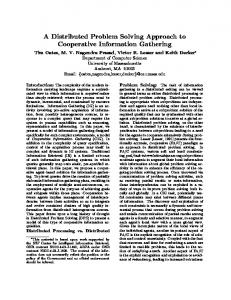
Figure 9. Phase transitions in the fraction of solvable problems and the average complexity for the channel scheduling problem using a complete backtracking algorithm

Figure 7. Solvable channel scheduling with small transmission radius (n = 7, C = 3, R = 0.40)

Figure 8. Unsolvable channel scheduling with large transmission radius (n = 7, C = 3, R = 0.55) The random access protocols that have been proposed for use in ad-hoc networks (e.g. ALOHA [1] and Busy Tone Multiple Access (BTMA) [19]) are useful for applications with bursty traffic conditions. In these protocols nodes share the same broadcast channel and transmit whenever they need to. The scheduled access techniques that have been proposed for ad-hoc networks [2], [15], [16] are better suited for non-bursty traffic conditions. In a typical scheduled access protocol, the available bandwidth is divided into multiple logical channels defined on the basis of differing time slots, frequency slots, spreading codes, or a combination thereof. Transmit power is limited so that a given logical channel can be simultaneously used by several nodes in the network so long as the nodes are suffi-

ciently far apart to limit mutual interference. This problem is also referred to in the literature as multi-hop TDMA or broadcast scheduling and is known to be NP-complete [16]. An excellent survey of the complexity results for this problem and analysis of some of the proposed suboptimal methods can be found in [12]. A simpler version of the broadcast scheduling problem, which is still NP-hard, can be defined as follows. Consider a wireless network consisting of n nodes, each of which transmits with the same power. We will assume that the transmission range of each node can be modelled as a circle of some radius R centered at the node. Let each node i in the network have a specified traffic need for ti contiguous time slots on a single channel (the time slots may be taken to be more general logical channels; we have adopted time slots for clarity). C channels are to be shared by all users in a given region. The goal is to find an assignment of ti time slots for each node i, such that no two neighboring nodes j and k share the same slot. The channel assignment problem can be easily modelled as a DCSP. Imagine each node as an agent, with ti multivalued variables {xi,1 , . . . xi,ti } for each agent i, corresponding to the allocated channels. These variables can take on values from 1 to C. The intra-agent constraint here is that each of the variables within an agent must take on distinct values. The inter-agent constraints take the form that if there are two neighboring (interfering) nodes i and j, their variables must not take on the same values. Formulated as a DCSP, this problem can be solved using one of the distributed backtracking algorithms described in the previous section. Although the communication and computational costs involved can be exponential in the number of nodes in the worst case, as we have discussed before, the average complexity can be within tolerable limits provided the system as a whole is under-constrained. Figure 7 shows a solvable instance of this problem on

0-7695-1435-9/02 $17.00 (c) 2002 IEEE

6

Proceedings of the 35th Hawaii International Conference on System Sciences - 2002

a small, sparse network. Variable assignments that satisfy all constraints are indicated in the figure. Figure 8, on the other hand, is an unsolvable instance of this problem on a dense network. Since there are only three channels available, and the nodes 2,3,4, and 5 form a clique of size 4, it is not possible for them to assign values to their respective variables without violating inter-agent constraints.

Figure 10. Average computational complexity of solving the channel scheduling problem for satisfiable instances using a randomized local search algorithm For a given mean traffic level per node, there are two parameters that affect the problem complexity and solvability: the transmission radius R, and the total number of channels available C. In order to study the effects of these parameters, we conducted the following experiment. 7 nodes are placed at random in a square region with unit sides. The transmission √ radius of all nodes is the same and is varied from 1 to 2. A particular combination of node positions and transmission radii corresponds to a unique network graph. A traffic level of 1 or 2 is generated at each node with equal probabilities. The bandwidth C is tested for values 4,6, and 8. 100 instances are generated for each value of transmission radius and bandwidth. A complete CSP-solver, similar to the DLL algorithm presented earlier in the paper, is used to obtain statistics on satisfiability and computational complexity of these instances. Figure 9 contains the results of these experiments, and shows that this problem undergoes a phase transition with respect to the Transmission Radius1 . These figures show that there is a critical value of the transmission radius below which a satisfying solution exists with high probability, and above which it exists with negligible probability. Figure 9 also shows the easy-hardeasy phase transition in average complexity when this con1 Note that in this problem the transmission radius increases with the ratio of constraints to variables. This is because for a given mean traffic level, number of nodes, and number of channels, the number of variables is fixed, and the number of constraints increases with the density of the network graph which in turn depends directly upon the transmission radius.

straint satisfaction problem is solved using a backtracking algorithm. It can be seen that when we increase the total number of channels – the bandwidth available to the system – the phase transition threshold moves to the right. This is intuitive, for adding bandwidth resources to this system makes it easier to provide a non-conflicting schedule to the nodes. Another experiment makes it clear that we can also expect some gains in complexity to result from the increase in bandwidth. If we restrict the study of complexity to only those instances in which there is a solution, i.e. satisfiable instances, then we can use a randomized local search algorithm to solve the problem. Figure 10 shows the normalized average cost for finding the satisfying solution for the three values of the bandwidth C ranging from 4 to 8. For each value of the transmission radius , the cost (which is a measure of the time taken to obtain the solution) is averaged over 300 runs of the local search algorithm, each starting from a random point in the search space. Figure 10 shows that an increase in bandwidth not only increases the probability that a solution, but also decreases the complexity of obtaining the solution when it exists.

4.2

Distributed Hamiltonian Cycle Formation

Consider the following task in a wireless sensor network: a set of nodes that form a connected network component wish to form a Hamiltonian cycle in a distributed manner. Recall that a Hamiltonian cycle in a graph is a cycle that visits each node in the graph exactly once. The formation of such a cycle is useful, for example, when forming a token ring in the network, and also forms the basis of some other distributed algorithms such as leader selection [13]. Another application is in optimal one-to-one broadcasting where nodes only send messages to one of their neighbors [17]. If a Hamiltonian cycle is established, any node in a one-to-one network can send a broadcast message to all the nodes in the network in sequential order, with a minimal number of data packets, and even get an acknowledgement/confirmation of the successful receipt of the message by all nodes. We can represent the problem of forming a Hamiltonian cycle as a DCSP as follows: Each of n nodes has an associated agent. Agent i has three multi-valued variables, F ROMi , T Oi , and HOP COU N Ti , representing the preceding and succeeding nodes in the hamiltonian cycle, and the number of hops from the beginning of the cycle respectively. The F ROMi and T Oi variables can take on values from 1 to n, while the HOP COU N Ti variable takes on values from 0 to n − 1. The intra-agent constraints pertaining to the F ROMi and T Oi variables is that they must be distinct and not equal to i. The following are the intraagent constraints pertaining to the HOP COU N Ti variable. Agent 1 is always considered to be the beginning point of the cycle, and hence HOP COU N T1 is always

0-7695-1435-9/02 $17.00 (c) 2002 IEEE

7

Proceedings of the 35th Hawaii International Conference on System Sciences - 2002

Figure 11. Unsolvable Hamiltonian cycle formation with small transmission radius (n = 7, R = 0.40)

Figure 12. Solvable Hamiltonian cycle formation with large transmission radius (n = 7, R = 0.55) equal to 0. The inter-agent constraints between agents i and j are that F ROMi = j if and only if i and j are neighbors and T Oj = i and HOP COU N Ti = (HOP COU N Tj + 1) mod n. Once it is specified in this manner, a complete DCSP algorithm can be used to solve this problem in a distributed manner. Figure 11 shows an unsolvable instance of this problem on a small, sparse network graph which contains no Hamiltonian cycles. No assignment of values to the variables of nodes 1, 6, and 7 will satisfy their respective intra-agent constraints, since they each have only one neighbor. Figure 12, on the other hand, shows a solvable instance of this problem on a denser network with a higher transmission radius. A particular solution is indicated in this figure using dashed lines, as are the corresponding constraint-satisfying values to the variables of each node agent. The transmission radii of the nodes is once again the factor affecting the complexity of this problem. Unlike in the medium access problem, however, the under-constrained region is reached by increasing the transmission radii of

Figure 13. Phase transitions in the fraction of solvable problems and the average complexity of forming a Hamiltonian cycle using a complete search algorithm with a simple pruning heuristic the nodes. This is because as the network graph becomes denser, the probability that a hamiltonian cycle exists in the graph increases. Figure 13 shows the phase transition in the probability of solution that occur in this problem as the transmission radius R increases. The figure is based on networks consisting of 7 randomly placed nodes in a square area with unit sides. 100 such instances were generated for each √ value of the transmission radius, which is varied from 1 to 2. The statistics for satisfiability and complexity of this problem were generated using a complete search algorithm with a simple pruning heuristic. Figure 13 also shows how the complexity for this problem too undergoes an easy-hardeasy phase transition. The graph density at which the phase transition occurs in this problem corresponds to a critical amount of per-node energy consumption. When sufficient energy resources are provided to the system, the problem enters the underconstrained regime where a solution exists with high probability and the solution complexity is low.

4.3

Partition into Coordinating Cliques

We now turn to a third and final problem that once again reflects the impact of transmission power on selfconfiguration. In wireless sensor network, sensing or other tasks may need to be distributed among the various nodes. One such example is in the task of monitoring the environment for a pre-specified phenomenon. If several nodes are selected to perform this task together, it is desirable that these nodes form a communication clique. In other words, any node in the coordinating group should be able to communicate directly over the wireless link with any other. For example, such a situation arises in the tracking of mobile nodes by Doppler radar sensors where it is required that a number of nodes participate and coordinate their actions jointly in order to track each mobile node [3]. The par-

0-7695-1435-9/02 $17.00 (c) 2002 IEEE

8

Proceedings of the 35th Hawaii International Conference on System Sciences - 2002

Figure 14. Unsolvable partition into coordinating cliques with small transmission radius (n = 9, k = 3, R = 0.40)

Figure 15. Solvable partition into coordinating cliques with large transmission radius (n = 7, k = 3, R = 0.55) titioning of the nodes has other applications in multi-hop wireless networks, such as in geography-informed energy conservation for routing [20]. We consider here the problem of arranging such communication cliques. Given n = q · k wireless nodes in the network, each with a transmitting radius R, the objective is to partition the network into q communicating cliques of size k each. This can be formulated as a DCSP as follows: Each node is an agent. Agent i has k − 1 variables {xi,1 , . . . xi,k−1 } which can each take on values from 1 to n. The values assumed by the variables must be distinct and no equal to i, as they are to represent the other members of the k-node clique. The inter-agent constraint between agents i and j is that one of agent i’s variables takes on the value j if and only if one of agent j’s variables is set to the value i, and all the other k − 2 variables of agents i and j share the same values. Also, one of agent i’s variable can be set to the value j if and only nodes i and j are neighbors.

Figure 16. Phase transitions in the fraction of solvable problems and the average complexity for the problem of partitioning a network into coordinating cliques using a complete search algorithm with a simple pruning heuristic. Figure 14 shows an unsolvable instance of this problem on a sparse network consisting of nine nodes which is to be partitioned into three coordinating cliques of size three each. This instance is clearly unsatisfiable because node 6 has only one neighbor and hence cannot communicate/coordinate with two other nodes. If we increase the transmission radius of each node, we get a denser network graph as shown in figure 15. This graph represents a solvable instance of the problem. The dashed edges represent one possible partition of the graph into three 3-cliques. Also shown in the figure is the corresponding, satisfiable, value assignment to the variables of each node agent. The problem of partitioning a graph into isomorphic subgraphs is known to be NP-hard for any connected subgraph with more than 3 nodes [9]. For a given set of nodes positioned arbitrarily, the difficulty of obtaining a partition in this problem is dependent on the density of the network graph. As we have seen before, this is affected directly by the transmission radii of the nodes. Figure 16 shows the phase transitions in both probability of partition and the average complexity for this problem based on 100 problem instances (n = 9, k = 3) for√each value of the transmission radius R ranging from 0 to 2. Once again, there is a critical transmission power level above which the problem has a solution with high probability and below which there is rarely a solution.

5

Conclusion

In this paper we studied the complexity of several problems related to the configuration of multi-hop wireless networks. In every instance, we saw that the existence of a solution and the difficulty of finding the solution exhibited a phase transition as the transmission radii of the nodes was varied. It followed that a certain critical range of resources was necessary to ensure that configuration problems in an

0-7695-1435-9/02 $17.00 (c) 2002 IEEE

9

Proceedings of the 35th Hawaii International Conference on System Sciences - 2002

multi-hop wireless network are tractable. The following design methodology is suggested by these results: • Use the phase transition analysis to determine the upper limit of the under-constrained region of the medium access scheduling problem. • Design the network to have a balance between transmission radii and the number of available logical channels that ensures that the design problem falls within the previously determined under-constrained region. • Having appropriately bounded the complexity of the problem, use stochastic search techniques to rapidly identify a good channel assignment. This final step can be incorporated into a self-configuring system, and repeated as necessary while the network is on-line. In general the configuration of an multi-hop wireless network is a multidimensional optimization problem. The goal is to identify the boundaries of the under-constrained region of the problem and then use efficient algorithms to identify solutions that fall within that region.

6

Acknowledgments

We are thankful to Dr. Carla Gomes and Dr. Bart Selman, Cornell University, for their guidance and support, and to Dr. Ivan Stojmenovic, University of Ottowa, and Jason Hill, U.C. Berkeley, for their helpful comments and suggestions for improving this paper.

[11] S. Kirkpatrick and B. Selman. Critical behavior in the satisfiability of random Boolean expressions. Science, 264(5163):1297–1301, 27 May 1994. [12] Errol L. Lloyd. Wireless Networks and Mobile Computing Handbook, Ed. Ivan Stojmenovic, chapter Broadcast Scheduling for TDMA in Wireless Multi-hop Networks. Wiley, 2001, to appear. [13] N.A. Lynch. Distributed Algorithms. Morgan Kaufmann Publishers, Inc., San Francisco, California., 1996. [14] D. Mitchell, B. Selman, and H. Levesque. Hard and easy distributions of sat problems, 1992. [15] L.C. Pond and V.O.K. Li. A distributed time-slot assignment protocol for mobile multi-hop broadcast packet radio networks. In MILCOM, pages 70–74, 1989. [16] R. Ramaswami and K.K. Parhi. Distributed scheduling of broadcasts in a radio network. In INFOCOM, pages 497–504, 1989. [17] Mahtab Seddigh, Julio Solano Gonzales, and Ivan Stojmenovic. RNG and internal node based broadcasting algorithms for wireless one-to-one networks. ACM Mobile Computing and Communications Review, 5(2):394–397, 2001, to appear. [18] Bart Selman, Henry A. Kautz, and Bram Cohen. Noise strategies for improving local search. In Proc. of the National Conference for Artificial Intelligence (AAAI’94), pages 337–343, 1994. [19] F.A. Tobagi and L. Kleinrock. Packet switching in radio channels, part ii: The hidden terminal in carrier sense multiple access and the busy-tone solution. IEEE Transactions on Communication, 23:1417–1453, 1975. [20] Ya Xu, John Heidemann, and Deoborah Estrin. Geographyinformed energy conservation for ad hoc routing. In Proc. of the Seventh Annual ACM/IEEE International Conference on Mobile Computing and Networking (ACM Mobicom), July 2001. [21] M. Yokoo, E. H. Durfee, T. Ishida, and K. Kuwabara. The distributed constraint satisfaction problem: Formalization and algorithms. IEEE Transactions on Knowledge and Data Engineering, 10(5):673–85, 1998.

References [1]

N. Abramson. The aloha system – another alternative for computer communications. In Proceedings of Fall Joint Computer Conference, 1970. [2] L. Bao and J. J. Garcia-Luna-Aceves. Collision-free topologydependent channel access scheduling. In MILCOM 2000. 21st Century Military Communications Conference Proceedings, pages 507– 511, 2000. [3] R. Bejar, B. Krishnamachari, C. Gomes, and B. Selman. Distributed constraint satisfaction in a wireless sensor tracking system. In Workshop on Distributed Constraint Reasoning, International Joint Conference on Artificial Intelligence, 2001. [4] P. Cheeseman, B. Kanefsky, and W. M. Taylor. Where the really hard problems are. IJCAI-91, 1:331–7, 1991. [5] Scott H. Clearwater, Bernardo A. Huberman, and Tad Hogg. Cooperative solution of constraint satisfaction problems. Science, 254:1181–1183, November 22 1991. [6] M. Davis, G. Logemann, and D. Loveland. A machine program for theorem-proving. Communications of the ACM, 5:394–397, 1962. [7] R. Dechter and D. Frost. Backtracking algorithms for constraint satisfaction problems. Technical report, http://www.ics.uci.edu/∼csp/r56-backtracking.pdf, Information and Computer Science Department, UC Irvine, 1999. [8] Deborah Estrin, Ramesh Govindan, John S. Heidemann, and Satish Kumar. Next century challenges: Scalable coordination in sensor networks. In Mobile Computing and Networking, pages 263–270, 1999. [9] M. R. Garey and D. S. Johnson. Computers and Intractability: A Guide to the Theory of NP-completeness. Freeman, San Francisco, 1979. [10] Y. Hamadi, C. Bessi`ere, and J. Quinqueton. Backtracking in distributed constraint networks. In Henri Prade, editor, Proceedings of the 13th European Conference on Artificial Intelligence (ECAI98), pages 219–223, Chichester, August 23–28 1998. John Wiley & Sons.

0-7695-1435-9/02 $17.00 (c) 2002 IEEE

10