They showed the convergence in presence of a modified update rule where the nearest neighbor value is scaled by a special time varying step size. A malicious.
Distributed protocol for determining when averaging consensus is reached Vikas Yadav, and Murti V Salapaka Abstract— Distributed averaging over a large network is a well studied problem that converges asymptotically; however, existing protocols does not provide a way for each node to distributively detect the occurrence of convergence. In this paper a method is developed to distributively determine when the consensus has reached within a given error margin. In absence of such a method all nodes in the network keep running the required computation and communication even if the consensus value are within acceptable tolerance, which is not preferable as in large-scale distributed networks resources like power are limited. Furthermore, this extra communication can cause signal interference with other critical information. This distributed detection takes finite time and occurs at each node simultaneously.
I. I NTRODUCTION Consensus or agreement in a large network of agents refers to the event in which each agent has same information. It is assumed that each node is sharing information with its neighbors. Averaging consensus is a special case where the each node starts with some initial node-value and as a result of agreement it obtains a value which is an average of initial node-values of all the nodes in the network. Averaging consensus protocol refers to the action to be performed on the received information. In this paper, the focus is on the linear averaging protocol presented in [10] where each node takes an average of the information received from neighboring nodes. [10] provides a necessary and sufficient condition that underlying network is strongly connected and balanced which leads to an asymptotic convergence in absence of any malicious user. It is shown in [12] that the requirement for balanced graph can be dropped by using weighted integrators in the protocol. A faster linear averaging protocol similar to [10] is proposed in [13]. In [2] a condition on functions that can be computed distributively is provided. A good survey of consensus problems is provided in [11], [9]. In [8] authors provide convergence analysis for the angular interaction among agents using a switched linear model. This model also assumes that over every finite period of time the particles are jointly connected for the length of the entire interval. Similar agrement problem over random graphs is addressed in [7] for graphs having binomial distribution. Most of these works assume some kind of connectivity in the network. In [3] work is done towards maintaining the connectivity of network by controlling the algebraic connectivity (also known as the second smallest eigenvalue of Laplacian of graph) of the network. In [6] authors address agreement problem over geometric random graphs with noisy Email: {vikasy, murti}@iastate.edu
communication. They showed the convergence in presence of a modified update rule where the nearest neighbor value is scaled by a special time varying step size. A malicious or faulty node is one which is not following the consensus protocol. In presence of such nodes, the averaging protocol becomes unstable, i.e. it fails to converge. In [1] authors provide results on stabilizing consensus protocol in presence of faults by assuming that node-values are binary. In large sensor networks, each node has limited power for its computational and communication need. In all consensus protocols, convergence takes place in asymptotic sense and there is no distributed way for each individual node to know if the convergence has reached within desired error margin. If each node can detect the consensus occurrence, then they can stop doing computation and communication required by the consensus protocol, and thus saving on the limited power supply. In this paper, a distributed algorithm is presented which facilitates each node to detect the occurrence of consensus within desired bounds in finite time. This algorithm requires implementation of maximum and minimum consensus protocols, which have finite convergence time bounded by the diameter of the network. The paper is organized as follows: In Section 2 a mathematical setup for the problem is presented with an overview of different protocols. In Section 3 the main scheme to achieve finite time convergence is presented. In Section 4 some examples are presented. Finally conclusion of the paper and discussion on future research directions is presented in Section 5. II. P ROBLEM SETUP Consider a system of N nodes or agents connected with each other in an arbitrary manner via communication links. Each node is sensing its local information e.g. local temperature or chemical concentration and is trying to compute the average of that local information over the whole network. The system is modelled as a graph G := (V, E) consisting of a set V := {1, 2, ..., N } of elements called vertices or nodes or agents, and a set E of node pairs called edges, with E ⊆ Ec := {(i, j)|i, j ∈ V }. If E = Ec i.e. each node is connected to rest of n − 1 nodes, it is called a complete graph. A graph is called undirected if for every pair of distinct nodes i and j both (i, j) and (j, i) are in E. Otherwise, it is called a directed graph or a digraph. A simple graph is a graph with no self loops, i.e. (i, j) 6∈ E if i = j. A graph is connected if it has a path between each pair of distinct nodes i and j, where by a path between nodes i and j we mean a sequence of distinct edges of G of the
form (i, k1 ), (k1 , k2 ), . . . , (km , j) ∈ E. A digraph is called “strongly connected” if there is a directed path between each pair of distinct nodes. Diameter D of a graph is the longest shortest path between any two pair of nodes. Fixed graphs are graphs in which the edge set E does not change with time. In this paper, fixed graphs are considered. Radius r of node pair (i, j) implies the minimum path length, i.e. the minimum number of edges connecting i to j is equal to r. The neighborhood Ni of ith node is a set consisting of all nodes within radius 1 not including the ith node itself. The degree or out-degree of an ith node is |Ni |, where |Ni | denotes the number of elements in Ni . The maximum degree of the graph is denoted by ∆ and the minimum degree of the graph is denoted by δ. The adjacency matrix A = {aij } of a graph G is an N × N matrix. ai,j > 0 only if the node pair (i, j) ∈ E and is equal to zero otherwise. The graph G is assumed to be simple, which implies that ai,i = 0 for all i = 1, 2, · · · N . The diagonal matrix Φ is anPN × N diagonal matrix with each N diagonal entry dii = j=1 aij . For undirected graph the graph Laplacian matrix L is defined as Φ − A. The graph Laplacian matrix L is an important function of the graph G. Eigenvalues of L have direct relation to the connectivity of the graph. Let, λ1 ≤ λ2 ≤ · · · λN be N eigenvalues of L. Since L has row sum equal to zero (such matrices are called row stochastic), λ1 = 0 is a trivial eigenvalue of L with ¯ 1 := [1, · · · , 1]T as the corresponding ¯ eigenvector i.e. L1 = 0. A graph is connected if and only if the second smallest eigenvalue of Laplacian is non-zero i.e. λ2 > 0 [4], and larger the λ2 better is the connectivity of the graph and faster is the convergence of the distributed consensus protocol. The second smallest eigenvalue λ2 is also called the algebraic connectivity of the graph. It is assumed that the communication among nodes is noiseless. A. Average consensus protocol The state vector of node-values for average consensus protocol is defined by column vector x(k) = (x1 (k) x2 (k) · · · xN (k))T . The average consensus protocol denoted by AP distributively computes the average of a given initial node-values x(0) = (x1 (0) x2 (0) · · · xN (0))T . It takes x(0) as an input and generates a sequence of nodevalues x(k)x(k) = (x1 (k) x2 (k) · · · xN (k))T such that {x(k)}∞ k=1 = AP (x(0)) based on the following nearestneighborhood update rule: X xi (k + 1) = xi (k) + � aij (xj (k) − xi (k)) (1) for all i = 1, 2 · · · N . This implies = P x(k)
The average protocol update rule can be rewritten as: xi (k + 1) =
N X
pij xj (k)
(3)
j=1
at ith node. Thus, each updated node-value is a weighted average of its neighboring node-values such that PNweights are non-negative and strictly less than one with j=1 pij = 1 for all i. This leads to the following conclusion: Proposition 2.2: xi (k + 1) ≤ max xj (k) for all i = 1, 2 · · · , N ;
(4)
xi (k + 1) ≥ min xj (k) for all i = 1, 2 · · · , N.
(5)
j
j
Equalities hold in above equations if and only if xi (k) = xj (k) for all i = 1, 2 · · · , N .
By taking maximum over all nodes in (4) (and minimum over all nodes in (5)) it can be shown that:
j∈Ni
x(k + 1)
1) P is row-stochastic non-negative matrix with a trivial eigenvalue of 1, 2) All eigenvalues of P are inside the unit circle, 3) If G is strongly connected then P is a primitive matrix, 4) If G is a balanced graph (¯1T L = 0) then P is columnstochastic (¯1T P = ¯1). Note that every undirected graph is a balanced graph. We will make following assumptions throughout the paper: 1 Assumption 2.1: (a) 0 < � < dmax , (b) the graph G is connected, and (c) if the graph G is directed graph, then it is “strongly connected” and balanced. The average consensus protocol for the graph G given by (1) converges asymptotically to average of the initial PN condition x(0) denoted by α := N1 i=1 xi (0) [9]. The average value α¯1 is an invariant quantity of the dynamics given by (1) i.e. P (α¯1) = α¯1. Further, this convergence is reached exponentially with exponent bounded above by µ2 , which is the second largest eigenvalue of P (µ2 < 1). Following property of P which relies on the fact that 0 < 1 is needed the rest of the development. � < dmax Proposition 2.1: Let pij be (i, j)th element of P . Then, 0 ≤ pij < 1 for all i, j = 1, 2 · · · N . Moreover, pii > 0 for all i. Proof: Since P is a non-negative matrix, it implies that 1 , 0 < pii = 1 − �dii < 1; and pij ≥ 0. Since, 0 < � < dmax aij for i 6= j, pij = �aij < dmax ≤ 1. Thus, pij < 1 for all i, j = 1, 2 · · · N with pii > 0 for all i. Also, for all j ∈ Ni , pij = �aij > 0.
(2)
where P = I − �L. Since I − �L ≈ exp(−�L), discrete time average consensus can be seen as the first order approximation of continuous time average consensus problem which is 1 given by x˙ = −�Lx. It is known that P with 0 < � < dmax , where dmax = max dii satisfies following properties [9]:
max x(k + 1) := max xj (k + 1) ≤ max xj (k)
(6)
min x(k + 1) := min xj (k + 1) ≥ min xj (k)
(7)
j
j
j
j
where equalities hold in both cases if and only if xi (k) = xj (k) for all i, j = 1, 2 · · · , N . Combining this with Proposition 2.2, it can be shown that node-value xi (k) at any time k is bounded from above by the maximum value in network
max x(k 0 ). The shortest distance between node i and j, denoted by d, is less than or equal to the diameter D of the graph. Let the path connecting i and j be min x(k 0 ) ≤ xi (k) ≤ max x(k 0 ) for all i = 1, 2 · · · , N . (8) (i, m ), (m , m ), . . . , (m , j). Because of weighted av1 1 2 d−1 0 0 eraging, at time k = k + 1, xm1 will become strictly less and for all k ≥ k . 0 than max x(k ) as shown below: The following lemma states that if a node reaches an average consensus protocol node-value that is strictly less N X than the maximum over the network at some past time instant xm1 (k 0 + 1) = pm1 n xn (k 0 ) k 0 then the node-value at that node at any future time instant n=1 X 0 k > k 0 remains strictly less than the maximum over the ≤ p x (k ) + pm1 n max x(k 0 ) m1 i i network at the past time instant k 0 . n6=i Lemma 2.1: Consider a graph G (undirected or directed 0 < pm1 i max x(k ) + (1 − pii ) max x(k 0 ) = max x(k 0 ). “strongly connected”, balanced graph) running an average consensus protocol AP given by (1) with an initial condition Thus, xm1 (k 0 + 1) < max x(k 0 ). Therefore, from Lemma x(k 0 ). Let, i and i0 be nodes such that xi (k) < max x(k 0 ) 2.1 for all k 00 ≥ k 0 + 1, xm1 (k 00 ) < max x(k 0 ). It follows and xi0 (k) > min x(k 0 ), respectively for some time instant that for all k 00 ≥ k 0 + 2, xm2 (k 00 ) < max x(k 0 ) and that k ≥ k 0 . Then for all k 00 ≥ k: for all k 00 ≥ k 0 + dij − 1, xj (k 00 ) < max x(k 0 ). Note that k 0 + D ≥ k 0 + dij − 1 (D ≥ dij ), therefore for all xi (k 00 ) < max x(k 0 ) k 00 ≥ k 0 + D, xj (k 00 ) < max x(k 0 ). xi0 (k 00 ) > min x(k 0 ) Proof: It is given that for node i, xi (k) < max x(k 0 ) Thus from lemma 2.2, after a finite time given by the for some time instant k ≥ k 0 . It follows that: diameter D of the graph, all node-values under averaging X consensus protocol become strictly less than the maximum xi (k + 1) = pij xj (k) value in network in the past and strictly greater than the j X minimum value in the network in the past, which in turn = pii xi (k) + pij xj (k) means that after a finite time the maximum value in the j6=i network decreases and the minimum value in the network X ≤ pii xi (k) + pij max x(k) increases. in the past and below by the minimum value in the network in the past. This can be expressed as follows:
j6=i
≤ pii xi (k) +
X
pij max x(k 0 ) [From Prop. 2.2]
j6=i
= pii xi (k) − pii max x(k 0 ) +
X
pij max x(k 0 )
j 0
= pii xi (k) + (1 − pii ) max x(k ) < pii max x(k 0 ) + (1 − pii ) max x(k 0 ) [∵ pii > 0] = max x(k 0 ). 0
Thus, xi (k + 1) < max x(k ). It follows that xi (k + J) < max x(k 0 ) for all J ≥ 1. Therefore, if node i assumes a node-value xi (k) < max x(k 0 ), then it remains strictly less than max x(k 0 ) for all future time instances. Similar proof holds for the minimum value case. Next lemma shows that after D time steps the maximum value has to strictly decrease and the minimum value has to strictly increase. Lemma 2.2: Consider a graph G (undirected or directed “strongly connected”, balanced graph) running an average consensus protocol AP given by (1) with an initial condition x(k 0 ) such that max x(k 0 ) > min x(k 0 ). Then for all k ≥ k 0 + D: max x(k) < max x(k 0 ), and (9) min x(k) > min x(k 0 ). (10) Proof: Consider any particular node j. There exists a node i such that xi (k 0 ) < max x(k 0 ) as min x(k 0 )
0 there exists K such that for all k ≥ K implies: |xi (k) − α| < � for all i = 1, 2, · · · N ⇒ −� < xi (k) − α < � for all i = 1, 2, · · · N ⇒ −� < max x(k) − α < � ⇒ | max x(k) − α| < � ⇒ lim max x(k) = α k→∞
Similarly, lim min x(k) = α k→∞
¯ = max xi (jD) and α(j) = min xi (jD). So, Now, α(j) they are subsequences of convergent sequences converging to same limit α, thus both α ¯ (j) and α(j) converge to α as ¯j → ∞. Further, note that β(j) = α ¯ (j) − α(j), therefore β(j) converges to 0 as j → ∞.
III. F INITE TIME CONVERGENCE WITHIN A GIVEN ERROR MARGIN
Consider the graph G = (V, E) with N nodes as defined above, each node running a distributed average consensus protocol AP given by (1). In this section, a distributed algorithm is provided which enables each node to detect the occurrence of the convergence in the network within a given error margin in finite time. To achieve this each node runs two more protocols, a maximum consensus protocol M XP and a minimum consensus protocol M N P given by (11) and (12) , respectively with z(k0 ) = y(k0 ) = x(k0 ), where k0 is the time when maximum and minimum protocols are started. By finite time convergence we imply that for any given ρ > 0, all agents can simultaneously reach to a decision in some finite time Tc that their node-values are ρ close to the desired average value i.e. they are in the interval [α−ρ, α+ρ]. From Proposition 2.2 and 2.3, we have that after time k = k0 + D, z(k) = max x(k0 )¯ 1 and y(k) = min x(k0 )¯1. Thus, at k = k0 + D the difference zi (k) − yi (k) will be same at each node. Define T (j) = (j − 1)D for j = 1, 2, · · · , as the set of time instants when M XP and M N P are reset. This is done at k = T (j) by setting their initial conditions z(T (j)) and y(T (j)) equal to the current node-values x(T (j)) from AP . Thus, at every time instant k = T (j + 1), M XP running at each node with initial value z(T (j)) will output max z(T (j)) and M N P running at each node with initial value y(T (j)) will output min y(T (j)). Define these outputs of M XP and M N P as α ¯ (j) = max z(T (j)), α(j) = min y(T (j)), respectively and the difference between these two outputs as β(j) = α ¯ (j)−α(j). At k = T (j +1) each node will have the same value β(j). Following corollary shows that α ¯ (j) and α(j) both converge to α, which in turn implies that β(j) converges to 0. Lemma 3.1: The sequences α ¯ (j) and α(j) converge to α as j → ∞. Further, the sequence β(j) converges to 0 as j → ∞.
This leads to the following distributed algorithm, which is the main result of the paper. It helps each node in deducing the occurrence of convergence in the network in finite time within desired error margin ρ. Algorithm I: Initialization: Given initial condition x(0), set z(0) = x(0) and y(0) = x(0). Start AP (x(0)), M XP (z(0)) and M N P (y(0)). Set j = 1. Step 1: At k = T (j) + D, let α ¯ (j) = M XP (z(T (j))), α(j) = M N P (y(T (j))) and β(j) = α ¯ (j) − α(j). Check at each node if β(j) < ρ; If yes then Stop, else set j = j + 1. Step 2: At k = T (j), set z(T (j)) = x(T (j)) and y(T (j)) = x(T (j)). Go to Step 1. Next theorem with help of Lemma 3.1 shows that the Algorithm I terminates in finite time. Theorem 3.1: Algorithm I terminates in some finite time Tc < ∞. Proof: β(j) converges to 0 as j → ∞ (from Lemma 3.1). Thus, for any given ρ > 0, there exists an integer j0 such that β(j) < ρ for all j ≥ j0 . This implies that the Algorithm I converges in finite time Tc = T (j0 ). The finite time Tc is not known beforehand because the size of β(j)’s which is proportional to the algebraic connectivity of the graph is not known to each node beforehand. The significant achievement is that all nodes can deduce in some finite time that the consensus in the network has reached and this happens at the same time at each node without help of any centralized information or source. Remark 1: In above algorithm, the maximum and minimum protocols are getting reset after every D time. The value of j at the termination of above algorithm gives number of times maximum and minimum protocols are executed. This number can be reduced at the cost of delaying the detection
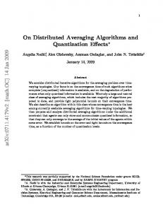
IV. E XAMPLES : F INITE TIME CONVERGENCE In this section, we present three scenarios of averaging protocol, and show how the algorithm presented in previous section facilitates distributed detection of occurrence of consensus in the network. Scenario A is of an undirected graph G1 with 25 nodes. The diameter of graph is 4, and the algebraic connectivity of the graph is 1.79. It has maximum degree of 12 and minimum degree of 2. The initial condition x(0) is chosen from a uniform distribution between +10 and − 10. The average value α = 0.95. Each node comes to know when the consensus has reached within an error margin of ρ = 0.02. The simulation result shown in Figure 1 demonstrates that after k = 45, each node correctly concludes that the convergence has occurred in the network within an error margin of 0.02. Scenario B is another undirected graph G2 with 25 nodes, diameter of the graph is 4, the algebraic connectivity of the graph is 1.48. It has maximum degree of 11 and minimum degree of 2. The average value α = −0.84. In this case, after consensus has reached and detected, there is some change in one of node-values at k = 60, so that the new average value becomes −0.65. The algorithm presented in previous section starts automatically to find another occurrence of convergence due to this change. The simulation result shown in Figure 2 demonstrates that each node comes to know when the consensus has reached within an error margin of 0.02 at k = 85. Scenario C is of a directed, strongly connected and balanced graph G3 with 25 nodes. The diameter of graph is 11 , and the algebraic connectivity of the graph is 0.17. It has maximum degree of 5 and minimum degree of 1. The initial condition x(0) is chosen from a uniform distribution between +10 and − 10. The average value α = 1.07. The
max−min−average with finite time convergence with given error margin of ρ=0.02
10
x(k) Averaging protocol z(k) Maximum protocol y(k) Minimum protocol
8
6
node−values x(k), y(k), z(k)
4 at k=45, each node decides that consensus has reached
2
0
−2
−4
−6
−8
−10
0
5
10
15
20
25 time k
30
35
40
45
50
Fig. 1. A: Maximum-minimum protocol running in parallel with averaging protocol helps individual agents to make a decision about the occurrence of agreement in the network
Max-min-average consensus in finite time within given error margin ρ = 0.02 10
8
6
4 node values x(k), y(k), z(k)
of convergence by choosing T (j) = (j − 1)D + ∆Tj where ∆Tj ≥ 0 for all j = 1, 2, · · · . One heuristic way to choose ∆Tj is by estimating the rate of decrease in the difference between maximum and minimum of node-values and setting ∆Tj equal to that estimated rate. In fact, above algorithm should work for all the graphs with diameter bounded by Dmax at the expense of delaying the detection of occurrence of convergence by time bounded by the difference between Dmax and actual diameter D. In other words, for this scheme to work it is not required for each node to know the actual diameter of the graph instead all it needs is some upper bound value on the diameter. In [5] a distributed method for computing the diameter of a graph is presented which uses a maximum of 2N 2 messages. Each node can first run this protocol to determine D in a distributed manner. Diameter D is the only parameter of the network graph required by each node. Remark 2: This detection of convergence technique can be generalized to distributed protocols such that x(k) satisfies Lemma 2.2, i.e. the maximum and minimum of x(k) over all nodes is strictly decreasing and increasing after every finite time D.
2
0
-2
-4
-6
-8
-10
0
10
20
30
40
50 time k
60
70
80
90
100
Fig. 2. B: One node changes it value at k = 60 after the agreement has reached in the network. Maximum-minimum protocol and averaging protocol restart to detect next occurrence of agreement in the network
simulation result shown in Figure 3 demonstrates that each node comes to know when the consensus has reached within an error margin of ρ = 0.02 at k = 96.
Max-min-average consensus in finite time withing given error margin ρ = 0.02 10
8
6
node values x(k), y(k), z(k)
4
2
0
-2
-4
-6
-8
-10
0
20
40
60 time k
80
100
120
Fig. 3. C: A case of directed graph. Maximum-minimum protocol running in parallel with averaging protocol helps individual agents to make a decision about the occurrence of agreement in the network
V. C ONCLUSIONS AND FUTURE WORK In this paper, a methodology is provided for detection of occurrence of consensus in the network running a distributed averaging protocol such that after finite time each node comes to know that the consensus has reached within given error bounds. This method requires two more protocols viz. maximum and minimum consensus protocols to run along with the averaging protocol at each sensor. The maximum and minimum protocols are reset after every D time which is the diameter of the graph. This is a conservative wait time, as mostly these protocols converge faster than D time. Thus, as part of future work this wait time can be further refined to a lower value such as period the graph. R EFERENCES [1] D. Angluin, M.J. Fischer, and H. Jiang. Stabilizing Consensus in Mobile Networks. Proc. International Conference on Distributed Computing in Sensor Systems (DCOSS06), June, 2006. [2] D. Bauso, L. Giarre, and R. Pesenti. Distributed Consensus in Networks of Dynamic Agents. Decision and Control, 2005 and 2005 European Control Conference. CDC-ECC’05. 44th IEEE Conference on, pages 7054–7059, 2005.
[3] M. C. DeGennaro and A. Jadbabaie. Decentralized control of connectivity for multi-agent systems. IEEE Conference on Decision and Control, San Diego, CA. December, 2006. [4] M. Fiedler. Algebraic connectivity of graphs. Czechoslovak Mathematical Journal, 23(98):298–305, 1973. [5] S. Haldar. An All Pairs Shortest Paths Distributed Algorithm Using 2n2Messages. Journal of Algorithms, 24(1):20–36, 1997. [6] Y. Hatano, A. K. Das, and M. Mesbahi. Agreement in presence of noise: Pseudogradients on random geometric networks. Proceedings of the 44th IEE Conference on Decision and Control, pages 6382–6387, Dec. 2005. [7] Y. Hatano and M. Mesbahi. Agreement over random networks. IEEE Trans. Autom. Contr., 50(11):1867–1872, Nov. 2005. [8] A. Jadbabaie, J. Lin, and A. S. Morse. Coordination of groups of mobile autonomous agents using nearest neighbor rules. IEEE Trans. Automat. Contr., 48(6):988–1001, 2003. [9] R. Olfati-Saber, J.A. Fax, and R.M. Murray. Consensus and cooperation in networked multi-agent systems. Proceedings of the IEEE, 95(1):215–233, 2007. [10] R. Olfati-Saber and R. M. Murray. Consensus protocols for network of dynamic agents. IEEE Trans. on Automatic Control, 49(9):1520–1533, Sept. 2004. [11] W. Ren, RW Beard, and EM Atkins. A survey of consensus problems in multi-agent coordination. American Control Conference, 2005. Proceedings of the 2005, pages 1859–1864, 2005. [12] C.W. Wu. Agreement and consensus problems in groups of autonomous agents with linear dynamics. Circuits and Systems, 2005. ISCAS 2005. IEEE International Symposium on, pages 292–295, 2005. [13] L. Xiao and S. Boyd. Fast linear iterations for distributed averaging. Decision and Control, 2003. Proceedings. 42nd IEEE Conference on, 5, 2003.