Distributed Quantum Computation Based-on Small Quantum Registers

Distributed Quantum Computation Based-on Small Quantum Registers Liang Jiang1 , Jacob M. Taylor1,2 , Anders S. Sørensen3 , Mikhail D. Lukin1 2

arXiv:0709.4539v2 [quant-ph] 21 Nov 2007

3

1 Department of Physics, Harvard University, Cambridge, Massachusetts 02138 Department of Physics, Massachusetts Institute of Technology, Cambridge, Massachusetts 02139 and Quantop and The Niels Bohr Institute, University of Copenhagen, DK-2100 Copenhagen Ø, Denmark (Dated: February 2, 2008)

We describe and analyze an efficient register-based hybrid quantum computation scheme. Our scheme is based on probabilistic, heralded optical connection among local five-qubit quantum registers. We assume high fidelity local unitary operations within each register, but the error probability for initialization, measurement, and entanglement generation can be very high (∼ 5%). We demonstrate that with a reasonable time overhead our scheme can achieve deterministic non-local coupling gates between arbitrary two registers with very high fidelity, limited only by the imperfections from the local unitary operation. We estimate the clock cycle and the effective error probability for implementation of quantum registers with ion-traps or nitrogen-vacancy (NV) centers. Our new scheme capitalizes on a new efficient two-level pumping scheme that in principle can create Bell pairs with arbitrarily high fidelity. We introduce a Markov chain model to study the stochastic process of entanglement pumping and map it to a deterministic process. Finally we discuss requirements for achieving fault-tolerant operation with our register-based hybrid scheme, and also present an alternative approach to fault-tolerant preparation of GHZ states.

I.

INTRODUCTION

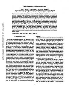
The key challenge in experimental quantum information science is to identify isolated quantum mechanical systems with good coherence properties that can be manipulated and coupled together in a scalable fashion. Recently, considerable advances have been made towards interfacing of individual qubits in the optical and microwave regimes. These include advances in cavity QED [1, 2] as well as in probabilistic techniques for entangling remote qubits [3, 4, 5]. At the same time, substantial progress has been made towards the physical implementation of few-qubit quantum registers using systems of coupled trapped ions [6, 7, 8], neutral atoms [9], or solidstate qubits based on either electronic and nuclear spins in semiconductors [10, 11, 12] or superconducting islands [13, 14]. While the precise manipulation of large, multi-qubit systems still remains an outstanding challenge, various approaches for connecting such few qubit sub-systems into large scale circuits have been investigated [5, 15, 16, 17, 18]. These studies suggest that hybrid schemes, which benefits from short range interactions for local coupling and (optical) long range interactions for non-local coupling, might be an effective way toward large scale quantum computation: small local few-qubit quantum systems may be controlled with very high precession using optimal control techniques [19, 20], and in practice it may be more feasible to operate several such small subsystems compared to the daunting task of high-precession control of a single large quantum system with thousands of qubits. Optical techniques for quantum communication can then be used to connect any two sub-systems. For example, we may directly transfer a quantum state from one sub-system to another via an optical channel [21] (see Fig. 1a), which immediately provides an efficient way to scale-up the total number of the physical

qubits we can manipulate coherently. In particular the use of optical means for connecting different subsystems has the advantage that it allows for fast non-local operations over large distances. This is advantageous for quantum error correction since the existence of such non-local coupling operations alleviates the threshold requirement for fault-tolerant quantum computation [22]. In practice, however, it is very difficult to have a perfect optical connection. In particular, there is excitation loss associated with the optical channel, due to scattering or absorption. For a lossy channel, it is therefore more desirable to use it to generate entanglement between different sub-systems (see Fig. 1b), rather than for direct state transfer. The entanglement generation is then heralded by the click patterns from the photon detectors. Such detection-based scheme is intrinsically robust against excitation loss in the channel, since it only reduces the success probability but does not affect the entanglement fidelity. This entanglement can then be used as a resource to teleport quantum state from one sub-system to another [23]. More generally, entanglement provides a physical resource to implement non-local unitary coupling gates (such as CNOT gate) [24, 25, 26, 27]. If there is only one physical qubit for each sub-system, so-called cluster states [28] can be created based on probabilistic, heralded entanglement generation (see Ref. [5] and references therein). Such cluster states can be used for universal quantum computation [29]. If there are two physical qubits available for each sub-system, cluster states can be created deterministically [30]; meanwhile one can also use these two-qubit sub-systems to implement any quantum circuit directly [4]. Furthermore, realistic optical channel connecting subsystems has other imperfections beside excitation loss, such as the distortion of the polarization or shape of the wave-packet. These imperfections will reduce the fidelity of the heralded entanglement generated between the sub-

2

FIG. 1: (Color online) Two schemes to couple different registers. (a) Deterministic state transfer from one register to the other [21]. (b) Probabilistic entanglement generation, heralded by distinct detector click patterns [3, 31, 32]. In the text, we argue that probabilistic, heralded entanglement generation is sufficient for deterministic distributed quantum computation.

systems. To overcome these imperfections in the channel, entanglement purification schemes have been proposed, which may create some high-fidelity Bell pairs from many low-fidelity ones [33, 34]. In particular, the entanglement pumping scheme originally presented in the context of quantum communication over long distances [31, 35, 36] provides a very efficient purification scheme in terms of local physical resources, and D¨ ur and Briegel [15] first proposed to use such entanglement pumping scheme for quantum computation. In principle, the infidelity of the purified Bell pair shared by the sub-systems can be very low, and is only limited by the error probability from local operations. In Ref. [15] it was found that three auxiliary qubits (requiring a total of five qubits including the storage and communication qubits) for each sub-system provide enough physical resources to obtain high fidelity entangled pairs via entanglement pumping. In order to implement the idea of distributed quantum computation using realistic optical channel and imperfect operations, it is necessary to consider the following questions: What are the minimal local physical resources needed for robust entanglement generation? What is the time overhead associated with entanglement generation? Can we extend the robustness to other imperfections, such as errors from initialization and measurement? Motivated by these considerations, we study the practical implementation of robust quantum registers for scalable applications. In Ref. [37] we have proposed an entanglement purification scheme that only requires two auxiliary qubits for robust entanglement generation. We have found that the time overhead associated with entanglement generation ranges from a factor of 10 to a few 100, depending on the initial and targeting infidelities. We have also suggested to use one more auxiliary qubit to suppress errors from initialization and measurement. Thus, our hybrid scheme also requires only 5 (or fewer)

qubits with local deterministic coupling, while providing additional improvements over the protocol of Ref. [15]: reduced measurement errors, higher fidelity, and more efficient entanglement purification. In this paper, we will provide a detailed discussion on the register-based, hybrid quantum computation scheme presented in Ref. [37]. The paper is organized as follows. In Sec. II, we will introduce the concept of quantum register and discuss two experimental implementations. In Sec. III, we will review the idea of universal quantum computation based on two-qubit quantum registers. In Sec. IV, we will specify the error models for imperfections and provide the basic ideas underlying our robust operations. In Sec. V, we will describe the robust measurement/initialization scheme. In Sec. VI, we will present our bit-phase twolevel entanglement pumping scheme. In Sec. VII, we will introduce the Markov chain model to quantitatively analyze the time overhead and residual infidelity associated with the stochastic process of entanglement pumping, and discuss further improvement upon our two-level entanglement pumping scheme. In Sec. VIII, we will map our stochastic, hybrid, and distributed quantum computation scheme to a deterministic computation model that is characterized by two quantities (the clock cycle and effective error probability), and estimate the practical values for these quantities. We will also consider the constraint set by the finite memory lifetime and determine the achievable performance of hybrid distributed quantum computation. Finally, in Sec. IX, we will discuss using our hybrid scheme for fault-tolerant quantum computation with quantum error correcting codes, and provide a resource-efficient approach for fault-tolerant preparation of the GHZ states.

II. QUANTUM REGISTER AND EXPERIMENTAL IMPLEMENTATIONS

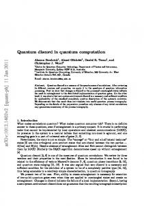
We define a quantum register as a few-qubit device (see Fig. 2a) that contains one communication qubit (c), with a photonic interface; one storage qubit (s), with very good coherence times; and several auxiliary qubits (a1 , a2 , ......), used for purification and error correction. A critical requirement for a quantum register is highfidelity unitary operations between the qubits within a register. The quantum registers considered here can be implemented in several physical systems, but in this paper we shall focus on two specific systems where these considerations are particularly relevant. First, ion traps have been used to demonstrate all essential elements of quantum registers. (1) The ion qubits may play the role of communication qubits: they can be initialized and measured efficiently using optical pumping and cycling transitions respectively, and they can also be prepared in highly entangled states with the polarization of single photons [39, 40]. Very recently, entanglement generation between ion qubits from two remote traps has been demonstrated

3

FIG. 2: (Color online) Distributed quantum computer. (a) Illustration of distributed quantum computer based on many quantum registers. Each register has five physical qubits, including one communication qubit (c), one storage qubit (s), and three auxiliary qubits (a1,2,3 ). Local operations for qubits within the same register have high fidelity. Entanglement between non-local registers can be generated probabilistically [3, 31, 32]. Devices of optical micro-eletro-mechanical systems (MEMS) [38] can efficiently route photons and couple arbitrary pair of registers. Detector array can simultaneously generate entanglement for many pairs of registers. (b) An ion trap coupled to a cavity also provides a promising candidate for distributed quantum computation. A single ion is resonantly coupled to the cavity and serves as the communication qubit; while the others can be storage or auxiliary qubits. (c) Nitrogen-vacancy (NV) defect center in photonic crystal micro-cavity. The inset shows the atomic structure of the NV center [10], which forms a quantum register. The electronic spin localized at the vacancy is optically accessible (measurement/initialization) and can play the role of the communication qubit. The nuclear spins from proximal 13 C atoms constitute the storage and auxiliary qubits, which are coherently controlled via hyperfine interaction and rf pulses.

tum computation only requires the coherence time to be approximately 104 times longer than the gate time, the very long coherence of the ions provides new opportunities, such as performing non-local coupling gates with some extra time overhead. (3) Coherent manipulation of few ions in the same trap has been demonstrated [45, 46], allowing gates to be implemented among the qubits in the register. (4) High fidelity operations between the ion qubits within the ion trap has also been demonstrated [19]. A second promising candidate for implementing quantum registers is the nitrogen vacancy (NV) centers in diamond. Each NV center can be regarded as an ion trap confined by the diamond crystal, which can be treated as a single register. The qubits for each NV register consists of one electronic spin associated with the defect and several nuclear spins associated with the proximal C-13 nuclei. The electronic spin is optically active, so that it can be measured and initialized optically. With optical cavities or diamond-based photonic crystal micro-cavities [47] one could enhance photon collection efficiency towards unity. Furthermore, the electron spin can be coherently manipulated by microwave pulses [10]. The electronic spin is thus suitable as the communication qubit. The nuclear spins are coupled to the electronic spin via hyperfine interactions. One can either use these hyperfine interaction to directly rotate the nuclear spins [48, 49], or apply radio-frequency pulses to address individual nuclear spins spectroscopically [50]. These nuclear spins have very long coherence times approaching seconds [12], and can be good storage and auxiliary qubits. Furthermore, the optical manipulation of the electronic spin can be well decoupled from the nuclear spins [51]. It can be inferred from the recent experiment [12] that the fidelity of local operations between electronic and nuclear spins is higher than 90%. While the fidelity is still low for the procedures considered here, we believe that it can be significantly improved (to higher than 0.999) by optimal control techniques [20, 50], such as composite pulses [52] and numerically optimized GRAPE pulses [53].

III.

[41, 42]. This experiment directly demonstrates the nonlocal connection required for our hybrid approach. Since the photon collection and detection efficiency is not perfect, the entanglement generation is a probabilistic process. However, the entanglement generation is also a heralded process, because different click patterns from the detectors can be used to identify each successful entanglement generation. As we will discuss Sec. III, such probabilistic, heralded entanglement generation process is already sufficient to implement deterministic non-local coupling gates. (2) The ion qubits can be good storage qubits as well. Coherence time of approximately 10 seconds has been demonstrated in ion traps [43, 44], which is 106∼7 times longer than the typical gate operation time which is at the order of µs. Since fault-tolerant quan-

UNIVERSAL QUANTUM COMPUTATION WITH TWO-QUBIT REGISTERS: FUNDAMENTALS

We now consider universal quantum computation via the simplest possible two-qubit registers [4, 30]. Each register has one qubit for communication and the other qubit for storage. We can use probabilistic approaches from quantum communication ([31] and references therein) to generate entanglement between communication qubits from two arbitrary non-local registers. The probabilistic entanglement generation creates a Bell pair conditioned on certain measurement outcomes, which are distinct from outcomes of unsuccessful entanglement generation. If the entanglement generation fails, it can be re-attempted until success, with an exponen-

4

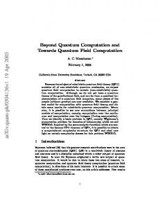
FIG. 3: (Color online) Quantum circuit for non-local CNOT gate between two ˛registers R1 and R2 . The √ circuit starts ¸ + ˛ with the Bell state Φ c1 ,c2 = (|00i + |11i) / 2 for the communication qubits c1 and c2 (the left blue box). After local unitary operations within each register (the middle orange boxes), qubits c1 and c2 are projectively measured in Z and X basis, respectively (the right green box). According to Eq. (1), up to some local unitary gates (the right green box), this circuit implements the non-local CNOT gate to qubits s1 and s2 from two quantum registers.

tially decreasing probability of continued failure. When the communication qubits (c1 and c2 ) are prepared in the Bell state, we can immediately perform the non-local CNOT gate on the storage qubits (s1 and s2 ) using gate-teleportation between registers R1 and R2 . The gate-teleportation circuit in Fig. 3 implements (before the conditional Pauli operations) the following map

 |φis1 ,s2 Φ+ c1 ,c2 → (σsz1 )mc2 (σsx2 )mc1 CNOTs1 ,s2 |φis1 ,s2 , (1) √ + where |Φ ic1 ,c2 = (|00i + |11i) / 2, CNOTi,j is the controlled-NOT (CNOT) gate with the ith qubit as control and the jth qubit as target, and mi = 0, 1 is the measurement result for qubit i from the circuit in Fig. 3. By consuming one Bell pair, one can implement any non-local controlled-U gate between two storage qubits [27], as shown in Fig. 4. Since operations on a single qubit can be performed within a register, the CNOT operation between different quantum registers is in principle sufficient for universal quantum computation [4]. Similar approaches are also known for deterministic generation of graph states [30] —an essential resource for one-way quantum computation [29]. We emphasize that deterministic entanglement generation is not required, which opens up a wide range of possibilities of entanglement generation. It is experimentally challenging to achieve deterministic quantum state transfer directly [21], but we are able to achieve the same task by probabilistic entanglement scheme and two-qubit quantum registers [4].

FIG. 4: (Color online) General circuit for non-local Controlled-U gate [27], with the storage qubit S 1 as control and the storage qubit S 2 as target. One Bell pair is consumed for this operation.

IV.

ERRORS AND IMPERFECTIONS

In practice, the qubit measurement, initialization, and entanglement generation can be noisy with error probabilities as high as ∼ 5%, due to practical limitations such as imperfect cycling transitions, finite collection efficiency, and poor interferometric stability. As a result, there will be a large error probability in non-local gate circuits. In contrast, local unitary operations may fail infrequently (pL . 10−4 ) when quantum control techniques for small quantum system are utilized [19, 20]. We now show that the most important sources of imperfections, such as imperfect initialization and measurement errors for individual qubits in each quantum register, and entanglement generation errors between registers, can be corrected with a modest increase in register size. We determine that with just three additional auxiliary qubits and high-fidelity local unitary operations, all these errors can be efficiently suppressed by repeated quantum non-demolition (QND) measurement [54] and entanglement purification [35, 36]. This provides an extension of Ref. [15] that mostly focused on suppressing errors from entanglement generation. We will use the following error model for the entire paper: (1) The imperfect local two-qubit operation Uij is † † Uij ρUij → (1 − pL ) Uij ρUij +

pL Trij [ρ] ⊗ Iij 4

(2)

where Trij [ρ] is the partial trace over the qubits i and j, and Iij is the identity operator for qubits i and j. This error model describes that with a probability 1 − pL the gates perform the correct operation and with a probability pL the gates produce a complete random output for the two involved qubits [71]. (2) The imperfect initialization of state |0i will prepare a mixed state ρ0 = (1 − pI ) |0i h0| + pI |1i h1| ,

(3)

which has error probability pI , i.e., it prepares the wrong state with a probability pI . (3) The imperfect measurement of state |0i will correspond to the projection oper-

5 ator P0 = (1 − pM ) |0i h0| + pM |1i h1| ,

(4)

This operator describes that a qubit prepared in state |0i or |1i will give rise to the opposite measurement output with the measurement error probability pM . (4) Finally, the entanglement fidelity for a non-ideal preparation of state |Φ+ i is defined as

 F = Φ + ρ Φ+ , (5) and the infidelity is just 1 − F . The fidelity does, however, not completely characterize the produced entangled state. Depending on the exact method used to generate the entangled state, one can in some situations argue that the error will predominantly be, e.g., only a phase error [3, 32, 55], whereas in other situations it will be a combination of phase and bit flip errors (see [31] and references therein). Below we shall therefore both consider the situation where we only have a dephasing error as well the situation, where we have a more complicated depolarizing error (exact definition given later). As we shall see, the knowledge that the error is of a particular type (e.g. only dephasing error) provides a significant advantage for purification. We will also assume a separation of error probabilities: any internal, unitary operation within the register fails with extremely low probability, pL , while all operations connecting the communication qubit to the outside world (initialization, measurement, and entanglement generation) fail with error probabilities that can be several orders of magnitude higher. pL  pI , pM , 1 − F.

(6)

In terms of these quantities the error probability in the non-local CNOT gate in Fig. 3 is pCN OT ∼ (1 − F ) + 2pL + 2pM .,

(7)

because we use one entangled state, two local operations, and two measurements. In the next two sections, we will show how to use robust operations to dramatically improve the fidelity for these non-local coupling gates. Robust measurement can be implemented by repeated QND measurement, i.e., a majority vote among the measurement outcomes (Fig. 5), following a sequence of CNOT operations between the auxiliary/storage qubit and the communication qubit. This also allows robust initialization by measurement. High-fidelity, robust entanglement generation is achieved via entanglement pumping [15, 35, 36] (Figs. 6 and 7), in which lower fidelity entanglement between the communication qubits is used to purify entanglement between the auxiliary qubits, which can then be used for non-local CNOT operations. To make the most efficient use of physical qubits, we introduce a new entanglement pumping scheme. In our bit-phase two-level entanglement pumping scheme, we first use unpurified Bell pairs to repeatedly pump (purify) against bit-errors (Fig. 7a), and then

FIG. 5: The robust measurement scheme based on repeated quantum non-demolition (QND) measurements and majority vote. Each QND measurement consists of initializing, coupling, and measuring the communication qubit. The QND measurements are repeated 2m + 1 times using the same communication qubit.

use the bit-purified Bell pairs to repeatedly pump against phase-errors (Fig. 7b). Entanglement pumping, like entanglement generation, is probabilistic; however, failures are detected. In computation, where each logical gate should be completed within the allocated time (clock cycle), failed entanglement pumping can lead to gate failure. To demonstrate the feasibility of our approach for quantum computation, we will analyze the time required for robust initialization, measurement and entanglement generation, and show that the failure probability for these procedures can be made sufficiently small with reasonable time overhead.

V.

ROBUST MEASUREMENT & INITIALIZATION

In this section, we will analyze the robust measurement scheme based on repeated QND measurement, discuss the recent experimental demonstration of robust measurement in the ion-trap system, and present two approaches to robust initialization. The measurement circuit shown in Fig. 5 yields the correct result based on a majority vote from 2m + 1 consecutive readouts (bit-verification). Since the evolution of the system (CNOT gate) commutes with the measured observable (Z operator) of the auxiliary/storage qubit, it is a quantum non-demolition (QND) measurement [54], which can be repeated many times. The error probability for such a majority vote measurement scheme is: εM ≈

2m+1 X j=m+1



2m + 1 j



j

(pI + pM ) +

2m + 1 pL 2

(8)

where the last term conservatively estimates the probability for bit-flip error of the auxiliary/storage qubit during the repeated QND measurement. For simplicity, we will use Eq. (8) for our conservative estimate of error probability for repeated QND measurement. Suppose pI = pM = 5%, we can achieve εM ≈ 8 × 10−4 by choosing m∗ = 6 for pL = 10−4 , or even εM ≈ 12 × 10−6 by choosing m∗ = 10 for pL = 10−6 . For convenience of discussion, we shall add εM to the set of imperfection parameters: (1 − F, pI , pM , pL , εM ). The time for robust

6 measurement is t˜M = (2m + 1) (tI + tL + tM ) .

(9)

where tI , tL , and tM are times for initialization, local unitary gate, and measurement, respectively. Measurements with very high fidelity (εM as low as 6 × 10−4 ) have recently been demonstrated in the iontrap system [56], using similar ideas as above. There are several possibilities to further improve the performance of the repeated QND measurement. (1) We may use maximum likelihood estimate (MLE) to replace the majority vote for repeated measurements with multi-value outcomes (e.g., fluorescent intensity) [56]. (2) We may keep updating the error probability using MLE after each measurement. Once the estimated error probability is below some fixed error rate, we stop the repetition of the QND measurement to avoid errors from redundant operations [56]. (3) We may use the implementation of CNOT gate that has small/vanishing bit-flip errors to the control qubit, which will reduce/eliminate the last term in Eq. (8). The robust measurement scheme also allows to achieve robust initialization by measurement, i.e., by measuring the state of a qubit with the robust measurement scheme, we initialize the qubit into the result of the measurement outcome with an effective initialization error εI ≈ εM .

(10)

Besides the above measurement-based scheme, we may achieve robust initialization using verificationbased scheme [72]. For clarity, we shall assume the measurement-based initialization [Eq. (10)] for the rest of the paper. VI.

ROBUST NON-LOCAL TWO-QUBIT GATE

With high-fidelity local unitary gate and repeated QND measurement, the error probability for non-local coupling gates (e.g., Fig. 3 and 4) is pCN OT ∼ (1 − F ) + 2pL + 2εM ,

FIG. 6: (Color online) Two-level entanglement pumping between registers Ri and Rj [circled by rounded rectangles in (a)]. (a,b) Generate and store one unpurified Bell pair. (c) Generate another unpurified Bell pair to pump (purify) the previously stored pair. (d) If the purification is successful, we obtain a purified Bell pair (level-1 pair) with higher fidelity; otherwise we discard the stored Bell pair and start the entire pumping process from the beginning. (e-f) The second level of entanglement pumping uses previously purified pairs to purify a stored Bell pair, to obtain a Bell pair with higher fidelity (level-2 pair).

A.

Entanglement pumping

We now consider entanglement pumping [31, 35, 36] with high-fidelity local unitary gate and robust measurement. During the entanglement pumping process, we first store one unpurified Bell pair [Fig. 6 (a,b)], and then generate another unpurified Bell pair to purify the previously stored pair [Fig. 6 (c,d)]. If the purification is successful, we will obtain a purified Bell pair with higher fidelity, which can be further purified by repeating the process in Fig. 6 (c,d) with new unpurified Bell pairs; otherwise we discard the stored Bell pair, and start the entire pumping process from the beginning. Sometimes, we may want to introduce a second level of entanglement pumping; that is to use previously purified pairs to purify a stored Bell pair [Fig. 6 (e-h)].

(11)

which is dominated by the infidelity of the Bell pair 1−F , since we assume pL ∼ εM  1−F . In this section, we will show how to create high-fidelity Bell pairs between two registers with a reasonable time overhead. We will first briefly review entanglement pumping [31, 35, 36]. Then we will quantitatively analyze the fidelity of the purified Bell pairs for our efficient two-level pumping scheme, and introduce the Markov chain model to calculate the failure probability for entanglement pumping within a given number of attempts. Next we will quantify the performance of the high-fidelity Bell pair generation in terms of the total error probability (or average infidelity) and the time overhead, and discuss the trade-off between these two criteria. Finally, we will mention a non-post-selective pumping scheme which may further reduce the time overhead.

B.

Fidelity of entanglement pumping

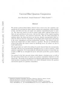
We now analyze the performance of entanglement pumping for different errors of the unpurified Bell pairs. If the unpurified Bell pair is dominated by one type of error (e.g., dephasing error with density matrix ρdephasing = diag [F, 1 − F, 0, 0] in the + Bell basis {|Φ√ i , |Φ− i , |Ψ+ i , |Ψ− i}, defined as |Φ± i = √ ± (|00i ± |11i) / 2, |Ψ i = (|01i ± |10i) / 2), we can skip the first level pumping. The unpurified pair then immediately becomes a level-1 pair and is purified with the circuit in Fig. 7b. In Fig. 8a we plot the fidelity curve (purified fidelity v.s. number of successful pumping steps) for the one-level pumping process (i.e. nb = 0), where a very high fidelity pair can be created after np = 3 suc-

7

FIG. 7: (Color online) Bit-phase two-level entanglement pumping scheme to create high fidelity entangled pairs between two registers Ri and Rj . (a) Circuit for the first level pumping to purify bit-errors, corresponding to Fig. 6c. (b) Circuit for the second level pumping to purify phase-errors, corresponding to Fig. 6g. The arrows indicate the time direction for each register. Robust measurements are used here. If the two outcomes are the same, it is a successful attempt of pumping; otherwise we generate new pairs and restart the pumping operation from the beginning.

cessful pumping steps. Note that we consider the full density matrix for all numerical calculation of entanglement fidelities [57], with the error models given in Eqs. (2,3,4). If the unpurified Bell pair contains errors from both bit-flip and dephasing processes (e.g., depolarizing error with density matrix ρdepolarizing =   1−F 1−F , , in the Bell basis), two-level endiag F, 1−F 3 3 3 tanglement pumping is needed. We introduce the following bit-phase two-level pumping scheme —the first level has nb steps of bit-error pumping using raw Bell pairs (Fig. 7a) to produce a bit-error-purified entangled pair, and the second level uses these bit-error-purified pairs for np steps of phase-error pumping (Fig. 7b). In Fig. 8b we plot the fidelity curves for the first level (thin blue curve) and the second level (thick red curve) of entanglement pumping. One-level pumping is insufficient to achieve high fidelity, but two-level pumping can achieve very high fidelity. With the parameters specified for Fig. 8b, the maximum fidelity is achieved
via the optimal choice of control parameters n∗b , n∗p = (1, 3) for successful pumping steps of the first and second levels, respectively. For successful purification, the infidelity of the purified (nb ,np ) pair, εE,infid , depends on both the control parameters (nb , np ) and the imperfection parameters (F, pL , εM ). For depolarizing error, we find 3 + 2np 4 + 2 (nb + np ) pL + (1 − F ) εM 4 3 (12)  nb +1  np +1 2 (1 − F ) (nb + 1) (1 − F ) + (np + 1) + 3 3 (n ≥1,np ≥1)

b εE,infid

≈

to leading order in pL and εM , for nb , np ≥ 1. The dependence on the initial infidelity 1 − F is exponentially suppressed at a cost of a linear increase of error from local operations pL and robust measurement εM . Measurement-related errors are suppressed by the pref-

FIG. 8: (Color online) Entanglement fidelity F as a function of the number of successful pumping steps. nb and np are the number of pumping steps used to purify bit-errors and phase-errors, respectively. We assume fixed measurement and local two-qubit gate error rates εM = pL = 10−4 . (a) For bit-flip ˛ ρ¸dephasing ˛ ¸ ˛ = diag ˘˛ ¸error ¸¯ [F, 1 − F, 0, 0] in the Bell basis ˛Φ+ , ˛Φ− , ˛Ψ+ , ˛Ψ− , with F = 0.95, onelevel entanglement pumping is sufficient. High fidelity of Ff in = 99.98% can be achieved by 3. (b) For ˜ deˆ np = 1−F , 3 , 1−F , with polarizing error ρdepolarizing = diag F, 1−F 3 3 F = 0.95, two-level entanglement pumping is needed (see text for more details). The first level pumping only purifies the bit-error, but accumulates the phase-error at the same time, and therefore the (thin blue) fidelity curve for the first level pumping drops for nb > 1. The second level (thick red curve) uses the purified level-1 pair (nb = 1) to pump another stored pair. High fidelity of Ff in = 99.97% can be achieved by np = 3. Note that we consider the full density matrix for all numerical calculation of entanglement fidelities [57], with the error models given in Eqs. (2,3,4).

actor 1 − F , since measurement error does not cause infidelity unless combined with other errors. In the limit of (nb ,np ) ideal operations (pL , εM → 0), the infidelity εE,infid can be arbitrarily close to zero, which is rigorously proved in Appendix A. On the other hand, if we use the standard entanglement pumping scheme [35, 36] (that alternates purification of bit and phase errors within each pumping level), the reduced infidelity from two-level pumping is 2 always larger than (1 − F ) /9. Therefore, for very small pL and εM , the new pumping scheme is crucial to minimize the number of qubits per register. (n ,n )

p b In Fig. 9, we show the contours of the infidelity εE,infid as a function of nb and np , where the contours are la(nb ,np ) beled by values of log10 εE,infid . The parameters for the contour plots are F = 0.90 (left) and F = 0.95 (right); εM = pL = 10−4 (up) and ε
M = pL = 10−6 (down). For optimal choice of n∗b , n∗p , the minimal infidelity is limited by εM and pL . For dephasing error, one level pumping is sufficient (i.e. no bit-error purification, nb = 0). The infidelity is approximately

(0,np ≥1)

εE

≈ (1 − F )

np +1

+

2 + np pL +2 (1 − F ) εM (13) 4

by expanding to the leading order in pL and εM .

8

(nb ,np ) FIG. 9: (Color online) The contours of the infidelity εE,infid as a function of nb and np for depolarizing error. We use (nb ,np ) log10 εE,infid to label the contours. The other parameters are F = 0.90 (left) and F = 0.95 (right); ε˜M = pL = 10−4 −6 and (down). With optimal choice of `(up) ´ ε˜M = pL = 10 n∗b , n∗p , the minimal infidelity is comparable to the corresponding value of pL .

VII.

MARKOV CHAIN MODEL

The overall success probability can be defined as the joint probability that all successive steps succeed. We use the model of finite-state Markov chain [58] to directly calculate the failure probability of (nb , np )-two-level entanglement pumping using Ntot raw Bell pairs, denoted (n ,n ) as εE,fb ailp (Ntot ).

A.

Markov chain model for entanglement pumping

We first use the Markov chain model to study the n-step one-level entanglement pumping. As shown in Fig. 10, we use ”0” to denote the initial state with no Bell pairs, ”1” for the state with one stored unpurified pair, (j + 1) for the state with one purified pair surviving j steps of pumping, and ”∗” for the final state with the purified pair surviving n steps of pumping. Altogether there are n + 2 states. The (success) transition probability from state j to state j + 1 is qj , while the (failure) transition probability from state j to state 0 is 1 − qj , for j = 0, 1, · · · , n. Here q0 ≡ 1 [corresponding to deterministic state transfer as shown in Fig. 6 (a,b)] and qj≥1

FIG. 10: (Color online) Markov chain model for one-level entanglement pumping. We use ”0” to denote the initial state with no Bell pairs, ”1” for the state with one stored unpurified pair, (j + 1) for the state with one purified pair surviving j steps of pumping, and ”∗” for the final state with the purified pair surviving n steps of pumping. The (success) transition probability from state j to state j + 1 is qj , while the (failure) transition probability from state j to state 0 is 1 − qj , for j = 0, 1, · · · , n. Here q0 ≡ 1 and qj≥1 can be calculated according to the density matrix of the purified Bell pair surviving j steps of pumping [36]. The final state is self-trapped, and goes back to itself with unit probability. Each transition attempt consumes one unpurified Bell pair.

can be calculated with the density matrix of the purified Bell pair surviving j − 1 steps of pumping [36]. The final state is self-trapped, and goes back to itself with unit probability, representing that once we have reached the desired final fidelity we no longer make any purification attempts and the system remains in this state with unit probability. Each transition attempt consumes one unpurified Bell pair. We would like to know the probability of reaching the final state ”∗” after Ntot attempts. More generally, we might also want to know the probability distribution over all n + 2 states. We use a (column) vector P~ with n + 2 elements to characterize the probability distribution among all n + 2 states. From the t-th attempt to the (t + 1)-th attempt, the probability vector evolves from P~t to P~t+1 according to the rule P~t+1 = M P~t , with the transition matrix   0 1 − q1 1 − q2 · · · 1 − qn 0 1  0   q1 0   M= . q2 0     ··· 0 qn 1

(14)

(15)

T Since the initial probability vector is P~0 = (1, 0, · · · , 0) , we can calculate the probability vector after Ntot attempts

P~Ntot = MNtot P~0 .

(16)

9

FIG. 11: (Color online) Markov chain model for two-level entanglement pumping. The required pumping steps are nb and np for the two levels, respectively. We use ”0, 0” to denote the initial state with no Bell pairs, ”0, j +1” for the state with one purified pair surviving j steps of pumping at the first level, ”k + 1, j + 1” for the state with one purified pair surviving k steps of pumping at the second level and one purified pair surviving j steps of pumping at the first level, ”k + 1, ∗” for the state with one purified pair surviving k steps of pumping at the second level and one purified pair surviving nb steps of pumping at the first level, and ”∗, 0” for the final state with one purified pair surviving np steps of pumping at the second level. For the first level pumping, the (success) transition probability from state ”k, j” to state ”k, j + 1” is qj , while the (failure) transition probability from state ”k, j” to state ”k, 0” is 1 − qj , for j = 0, 1, · · · , nb . For the second level pumping, the (success) transition probability from state ”k, ∗” to state ”k +1, 0” is Qk , while the (failure) transition probability from state ”k, ∗” to state ”0, 0” is 1 − Qk , for k = 0, 1, · · · , np . The final state is self-trapped, and goes back to itself with unit probability.

The probability vector P~Ntot describes the entire probability distribution over all states of the Markov chain. The last element of P~Ntot is the success probability of reaching the final state ”∗” after Ntot attempts; the failure probability after Ntot attempts is thus (n ,n )

εE,fb ailp (Ntot ) = 1 − (PNtot )n+2 .

(17)

For two-level entanglement pumping, the state transition diagram is shown in Fig. 11. nb and np are the number of pumping steps used to purify bit-errors and phaseerrors, respectively. As detailed in Appendix B, we may use a (column) vector P~ with (nb + 1) (np + 1) + 1 elements to characterize the probability distribution among all (nb + 1) (np + 1) + 1 states. From the t-th attempt to the (t + 1)-th attempt, the probability vector evolves from P~ (t) to P~ (t + 1) according to the same rule as above [Eq. (14)], but with the transition matrix M given in Eq. (B2). Similar to one-level pumping, we can calculate the probability vector after Ntot attempts using Eq. (16). The probability vector P~Ntot describes the entire probability distribution over all states of the Markov chain.

FIG. 12: (Color online) Failure probability εE,fail as a function of Ntot . We assume a depolarizing error with F = 0.95, pL = ε˜M = 10−4 . We choose (nb , np ) = (2, 3) for the lower curve, and (3, 4) for the upper curve. For large Ntot , the failure probability εE,fail decreases exponentially with Ntot .

The last element of P~Ntot is the success probability of reaching the final state ”∗, 0” after Ntot attempts; the failure probability after Ntot attempts is then (n ,n )

p b εE,fail (Ntot ) = 1 − P (Ntot )(nb +1)(np +1)+1 .

(18)

(n ,n )

p b In Fig. 12, we plot the failure probability εE,fail (Ntot ) v.s. Ntot , for control parameters (nb , np ) = (2, 3) and (3, 4). For Ntot sufficiently large, the failure probability decreases exponentially to zero. For any given parameters, we can efficiently suppress the failure probability with some reasonably large Ntot .

B.

Total error probability & average infidelity

We now introduce the total error probability (TEP) approximated by the sum of the failure probability and the infidelity of the purified Bell pair (n ,np )

εE b

(n ,n )

(n ,n )

p p b b (Ntot ) ≈ εE,fail (Ntot ) + εE,infid .

(19)

This is a very conservative estimate, since sometimes we do create some partially purified Bell pair though not the targeted purified Bell pair. And here we just say that the state has fidelity zero in these cases. To consider the possibility of using a partially purified Bell pair for output, we may introduce another useful quantity —the average infidelity (AIF) —for the output Bell pair from the robust entanglement generation, where we take into account these partially purified pairs. The average infidelity of the output pair is the weighted average of the infidelity of the Markov chain (n ,np )

δE b

(Ntot ) D E (nb ,np ) ≡ 1 − FNtot np

=

(20)

nb X X 1 (n0b ,n0p ) εE,infid P (Ntot )(nb +1)n0p +n0 +2 + P (Ntot )1 . b 2 0 0

nb =0 np =0

10 which is achieved by the control parameters
(nb , np ) ≡ n∗b , n∗p , for the imperfection parameters {pL , 1 − F, εM }. We remark that a faster and less resource intensive approach may be used if the unpurified Bell pair is dominated by dephasing error. Then, one-level pumping is sufficient (i.e. no bit-error purification, nb = 0). The optimized total error probability and average infidelity (thin blue curves) for this situation are plotted as a function of Ntot in Fig. 13.

C.

FIG. 13: (Color online) The optimized total error probability εE [Eq. (21)] (upper plots) and the optimized average infidelity δE [Eq. (22)] (lower plots) as a function Ntot . The error probability for the local coupling gates is pL = 10−4 (left plots) and pL = 10−6 (right plots). One-level pumping is used for dephasing error (thin blue curves); two-level pumping is used for depolarizing error (thick red curves). The other parameters F = 0.95, pI = pM = 5% are the same for all plots. Both εE and δE saturate for large Ntot . In each plot, we also show the initial infidelity 1 − F (upper blue dashed lines) and the local error probability pL (lower violet dashed lines).

Here the first term sums over all states of the Markov chain (except for the initial one), each of which has at (n0b ,n0p ) least one partially purified pair with infidelity εE,infid and probability P (Ntot )(nb +1)n0p +n0 +2 ; the last term b comes from the situation that none of the partially purified Bell pairs remain after the last attempt of the entanglement purification and we just use a classically correlated pair with infidelity 1/2. Generally, the average infidelity is smaller than the total error probability. We may also optimize the choice of the control parameters (nb , np ) (n ,np )

εE (Ntot ) ≡ min εE b (nb ,np )

(Ntot )

(n ,np )

(nb ,np )

(Ntot ) .

(22)

In Fig. 13, we plot both the optimized total error probability εE and the optimized average infidelity δE as a function of Ntot . Both quantities asymptotically approaches the same minimum value εE (Ntot ) =

lim

Ntot →∞


t˜E ≈ hNtot i × tE + tL + t˜M ,

δE (Ntot ) = ∆min .

(23)

Here the minimum value is simply the minimal infidelity of the entanglement purification (n ,n )

p b ∆min ≡ min εE,infid

(nb ,np )

(25)

where tE is the average generation time of the unpurified Bell pair. Note that the entanglement generation itself is a stochastic process. In principle, we may also include the stochastic nature of the entanglement generation by introducing a sub-level of Markov chain to characterize the stochastic entanglement generation. Since each entanglement generation either succeeds or fails, the sub-level Markov chain only involves two states, which can be easily incorporated into the Markov chain models discussed above. After incorporating the sub-level into the Markov chain, each transition corresponds to one attempt of entanglement generation, instead of one attempt of entanglement purification that consumes one unpurified Bell pair previously. Nevertheless, the number of Bell pairs generated in a given period of time (i.e. Ntot ) has a distribution. Since −1/2 the relative deviation of this distribution (∼ Ntot ) is fairly small for large Ntot (> 20), this only has a minor influence. Thus we replace hNtot i by Ntot .

D.

δE (Ntot ) ≡ min δE b

lim

The total time for robust entanglement generation t˜E is proportional to the average number of raw Bell pairs generated hNtot i

(21)

and

Ntot →∞

Total time for robust entanglement generation

(24)

Trade-off between gate quality and time overhead

We now consider the balance between the ”quality” of the robustly generated entangled pairs and the time overhead Ntot associated with the robust generation process. We may use either the optimized total error probability εE (Ntot ) or the optimized average infidelity δE (Ntot ) to characterize the quality. Since both quantities approaches the same asymptotic minimum ∆min according to Eq. (23), there is only little improvement in the quality of the robust entanglement generation once εE (Ntot ) or δE (Ntot ) is comparable to ∆min (say 2∆min ). Thus, we find the value for Ntot by imposing the relations εE (Ntot ) = 2∆min

(26)

11

FIG. 14: (Color online) Contours of the total error probability εE (or average infidelity δE ) after purification (left), the total number of unpurified Bell pairs Ntot associated with εE [Eq. (26)] (middle), and Ntot associated with δE [Eq. (27)] (right). The contours are drawn with respect to the imperfection parameters pL (horizontal axis) and F (vertical axis). Two-level pumping (up) is used for depolarizing error, and one-level pumping (down) for dephasing error. pI = pM = 5% is assumed.

or δE (Ntot ) = 2∆min .

(27)

First, we consider the total error probability εE (Ntot ). The relation in Eq. (26) can be simplified, if
we assume fixed control parameters (nb , np ) ≡ n∗b , n∗p for the left hand side (rather than minimizing over all possible choices of (nb , np )). Combined with Eq. (19), the failure probability should be comparable to the minimal infidelity (n∗b ,n∗p ) εE,fail (Ntot ) ≈ ∆min .

(28)
Since both the variable ∆min and the parameters n∗b , n∗p depend on {pL , pI , pM , 1 − F }, the above relation implicitly determines Ntot as a function a function of {pL , pI , pM , 1 − F }. In Fig. 14, we plot the contours of εE [Eq. (26)] and Ntot [Eq. (28)] with respect to the imperfection parameters pL and 1 − F , while assuming pI = pM = 5%. Actually the choice of pI and pM (< 10%) has negligible effect on the contours, since they only modify εM marginally. For initial fidelity F0 > 0.95, the contours of εE are very close to vertical lines; that is εE is mostly limited by pL with an overhead factor (about 10) very insensitive to F0 . The contours of Ntot indicate that the entanglement pumping needs about tens or hundreds of raw Bell pairs to ensure a very high success probability.

Similarly, we may also numerically obtain the value Ntot from Eq. (27). The contour plot of Ntot with respect to the imperfection parameters pL and 1 − F is also shown in Fig. 14 (c,f). We compare Ntot s obtained from two estimates (total error probability [Eq. (26)] and average infidelity [Eq. (27)]). As we expected, the Ntot obtained from total error probability is approximately 1.2 ∼ 2 time larger than the Ntot obtained from average infidelity, since the former is a more conservative estimate and requires more unpurified Bell pairs. Nevertheless, the difference is small and can be easily accounted by a prefactor of order unity. For clarity, in the rest of the paper we will use the Ntot estimated by using total error probability, and sometimes quote the values estimated by using average infidelity.

E.

Entanglement pumping with non-post-selective (NPS) scheme

We now consider another entanglement pumping protocol, proposed by Campbell [59]. The entanglement pumping scheme we have considered so far is postselective (PS); that is we discard the Bell pair if one step of entanglement pumping is not successful. However, the Bell pair may still be highly entangled even if the entanglement pumping failed at some intermediate step. The non-post-selective (NPS) entanglement pumping scheme

12

FIG. 15: (Color online) Markov chain model for one-level entanglement pumping with non-post-selective (NPS) scheme. The key difference from the previous Markov chain model with post-selective (PS) pumping scheme (see Fig. 10) is that here the transition for unsuccessful pumping reduces the chain label (score) by 1, while in the previous model the transition for unsuccessful pumping goes back to state ”0” (restart of the entire pumping scheme).

[59] keeps track of the evolution of the density matrix of the Bell pair after each step of pumping. The NPS scheme avoids the inefficient restart (i.e., discarding intermediately purified Bell pairs), and it may reduce the time overhead, especially when the unpurified Bell pairs have relatively low fidelity (F < 0.9). In Ref. [59], the NPS pumping is discussed in the context of generating a graph state. We now describe how to use the NPS pumping scheme to generate purified Bell pairs. To simplify the discussion, we first assume that the errors from local measurements and operations are negligible. This assumption enables us to establish a connection between the Markov chain model and the NPS pumping scheme. Suppose the unpurified Bell pairs have only phase errors, then one level of entanglement pumping is sufficient. For this error model, one can show that a failed attempt produces an EPR pair with a density matrix identical to the one in the previous step [59]. One may introduce an accumulated score associated with entanglement pumping. The score increases by one unit for each attempt of successful pumping, and decrease by one unit for an attempt of unsuccessful pumping. The score for no Bell pair is 0, and for one unpurified Bell pair it is 1. The score exactly corresponds to the state label of the Markov chain (see Fig. 15). After each attempt of pumping, the score changes by ±1. If the score drops to 0 (i.e. no Bell pair left), it gets back to 1 in the next attempt (i.e., creating a new unpurified Bell pair). The pumping procedure continues, until the score reaches n + 1 (i.e., the final state ”∗” in the Markov chain). The key different from the previous Markov chain for post-selective pumping scheme (see Fig. 10) is that here the score decrease by 1 for unsuccessful pumping rather than restart from 0. This modification increases the success probability of the robust entanglement generation.

FIG. 16: (Color online) Markov chain model for two-level entanglement pumping with NPS scheme. We still use PS entanglement pumping scheme at the first level to have minimal accumulation of phase errors. Only at the second level, does the NPS scheme work more efficiently than the original PS scheme (see Fig. 11).

When the unpurified Bell pairs have both bit-flip and phase errors (e.g., depolarizing error), we may use the bitphase two-level pumping scheme (see Sec. VI B), which purifies the bit error at the first level and then the phase error at the second level. Since the phase error is not purified at the first level, it accumulates after each attempt of pumping. Therefore, it is better to use PS entanglement pumping scheme at the first level to have minimal accumulation of phase errors. At the second level, the NPS scheme works more efficiently than the PS scheme. The Markov chain circuit for such mixed PS-NPS pumping schemes is shown in Fig. 16. In practice, the error probability for the local operations is always finite. Then our simple Markov chain model only provides an approximate description for the real process. The approximation comes from the fact that the score is now insufficient to specify the density matrix for intermediate Bell pairs, in the presence of local operational errors. In order to obtain the density matrix for the intermediate state, we need to have the entire list of all previous pumping outcomes. Nevertheless, when the local operational errors are small compared to the infidelity of the intermediate Bell pairs, the Markov chain model still provides an (optimistic) estimate for the total error probability and the average fidelity. We now compare the Ntot s associated with the PS and NPS schemes. The contours of the ratio between the two Ntot s is plotted as a function of pL and F in Fig. 17. As pointed out in Ref. [59], there is a significant improvement by using the NPS scheme (more than a factor of 3), for F < 0.9 and pL < 10−4 .

13 with a photon collection/detection efficiency η, vacuum radiative lifetime τ , and the cooperativity (Purcell) factor C for cavity-enhanced radiative decay [60, 61]. Eq. (31) is obtained from the estimate for the meaN surement error probability pM ≈ (1 − η) photon with Nphoton ≈ tM / (τ /C). We assume that the entanglement is generated based on detection of two photons [3, 32], which takes time tE ≈ (tI + τ /C) /η 2 .

FIG. 17: (Color online) The contours for the ratio between Ntot associated with the post-selective (PS) scheme and Ntot associated with the non-post-selective (NPS) scheme, as a function of pL and F . For both schemes, we use the same formula [Eq. (27)], but different Markov chain models (Fig. 10 and 15). The improvement from the NPS scheme becomes significant (more than a factor of 3), for F < 0.9 and pL < 10−4 .

VIII.

MAPPING TO DETERMINISTIC MODEL

In this section, we will map our stochastic, hybrid, and distributed quantum computation scheme to a deterministic computation model, which is characterized by two parameters — the clock cycle and the effective error probability. We will show that even when the underlying operations such as the entanglement generation are non-deterministic, our approach still maintains reasonable fast clock cycle time and sufficiently low effective error probability. We will associate our discussion with achievable experimental parameters, consider the constraint set by the finite memory lifetime, and determine the achievable performance of hybrid distributed quantum computation.

Generally entanglement fidelity is higher for the twophoton schemes than one-photon schemes [31]. In addition, some two-photon schemes have intrinsic purification against bit-flip errors [55]. The time for robust measurement is given in Eq. (9), and the total time for robust entanglement generation is given in Eq. (25). Combining Eqs. (29), (31), (32), (9) and (25), we obtain the clock cycle time (in units of the local operation time) as a function of other parameters   tC τ , pM , η, m, Ntot . =f (33) tL tL C Meanwhile, we may obtain the relation m = m [pL , pI , pM ] by minimizing εM with Eq. (8), and find the relation Ntot = Ntot [pL , F, εM ] = Ntot [pL , F, 2∆min [pL , pI , pM ]] using Eqs. (24 and 26). Therefore, we have   tC τ , pM , η, pL , F . (34) =f tL tL C The dimensionless parameter is the ratio between the times of emitting a single photon and performing a local unitary operation. For systems such as ion-traps and NV centers, this ratio is usually much less than unity (< 0.01). Similarly, we can obtain the effective error probability in terms of imperfection parameters γ = g [pL , pM , F ] ,

A.

Time and error in the theoretical model

All the previous discussions can be summarized in terms of the clock cycle time tC = t˜E + 2tL + t˜M ≈ t˜E ,

(29)

and the effective error probability γ = εE + 2pL + 2εM ,

(30)

for a general coupling gate between two registers. We now provide an estimate of the clock cycle time based on realistic parameters. The time for optical initialization/measurement is tI = tM ≈

ln pM τ , ln (1 − η) C

(31)

(32)

(35)

by combining Eqs. (8), (30) and (26). In Fig. 18, we plot the clock cycle time tC and effective error probability γ, for two-level pumping against depolarizing error. Assuming η = 0.2, we consider the two choices of parameters 1 − F = pI = pM = 5% (left) and 1% (right). For each case, we plot the contours of the normalized clock cycle time tC /tL as a function of pL and tLτC , and the effective error probability γ as a function of pL . The clock cycle time can be reduced by having a fast radiative decay rate τ /C, which can be facilitated by having a large cooperativity factor C. The reduction of the clock cycle time stops once this ratio is below certain value, approximately 0.003 (left) and 0.001 (right), where local gate operation becomes the dominant time consuming step. Similarly, we plot the clock cycle time tC and effective error probability γ, for one-level pumping against dephasing error in Fig. 19.

14

FIG. 18: (Color online) Plots of clock cycle time tC and effective error probability γ, for two-level pumping against depolarizing errors. Upper plots: contours of the normalized clock cycle time tC /tL (upper) as a function of pL and tLτC (the normalized effective radiative lifetime). Lower plots: the effective error probability γ as a function of pL . We assume 1 − F = pI = pM = 5% (left) and 1% (right), and η = 0.2.

FIG. 19: (Color online) Plots of clock cycle time tC and effective error probability γ, for one-level pumping against dephasing error. Upper plots: contours of the normalized clock cycle time tC /tL (upper) as a function of pL and tLτC (the normalized effective radiative lifetime). Lower plots: the effective error probability γ as a function of pL . We assume 1 − F = pI = pM = 5% (left) and 1% (right). And η = 0.2.

In the limit of negligible radiative decay time, we obtain the lower bound for the normalized clock cycle time

memory error probability for each clock cycle is approximately tC /tmem , which should be small (say 10−4 ) in order to achieve fault-tolerant quantum computation. This is indeed the case for both trapped ions (where tmem ∼ 10 s has been demonstrated [43, 44]), as well as for proximal nuclear spins of NV centers (where tmem approaching a second can be inferred [12]). So far, we have justified the feasibility of the hybrid distributed quantum computation scheme. In the next subsection, we will provide a criterion for hybrid distributed quantum computation.

 lim tC /tL = τ tL

C →0

Ntot for m = 0 , (2m + 2) Ntot for m ≥ 1

(36)

where for m ≥ 1 there is a time overhead 2m + 2 associated with local operation and robust measurement; while there is no such overhead for m = 0.

B.

Estimated numbers for experimental setups C.

Suppose the parameters are (tL , τ, η, C) = (0.1 µs, 10 ns, 0.2, 10) [62, 63, 64] and
(1 − F, pI , pM , pL , εM ) = 5%, 5%, 5%, 10−4 , 8 × 10−4 for our quantum registers (based on ion-traps or NV centers). For depolarizing errors, two-level pumping
can achieve (tC ,γ) = 200 µs, 2.7 × 10−3 . For some entanglement generation schemes [3, 32, 55] in principle only dephasing error exists, because they have intrinsic purification against bit-flip errors. If all bit-flip errors are suppressed, then one-level
pumping is sufficient and (tC ,γ) = 42 µs, 2.2 × 10−3 [74]. In Table I, we have listed (tC ,γ) for parameters 1 − F = pM = pI = 5% or 1%, and pL = 10−3 , 10−4 , 10−5 , or 10−6 . As expected, we find that tC gets longer, if the fidelity F is lower and/or the error probability (pM or pI ) is higher; tC significantly reduces if the error for the unpurified Bell pairs changes from depolarizing error to dephasing error. We remark that tC should be much shorter than the memory time of the storage qubit, tmem . Because the

Constraints from finite memory life time

Above we have mostly ignored the effect of finite memory time, and with the various sequences of purification of imperfections the final fidelity of the operations have then been limited only be the local operation. All of these purifications, however, increase the time of the operations and eventually the system may become limited by the finite life time of the memory. In this subsection we shall evaluate this constraint set by the finite memory lifetime. To simplify the discussion we assume that we have a very short radiative lifetime τ or that we are able to achieve a very large Purcell factor so that τ /C becomes negligible. All the time scales are then proportional to the local gate time tL . With a finite memory time, i.e., some fixed tmem /tL , there is a limit to have many operations we can do before we are limited by the memory error. To get an estimate for this limit we assume that the ideal number of operations is roughly given by the

15

pL pL pL pL

= 10−3 = 10−4 = 10−5 = 10−6

Depolarizing F = 0.95 F = 0.99 tC (µs) γ tC (µs) γ 65 1.9 × 10−2 19 9.1 × 10−3 200 2.7 × 10−3 49 1.2 × 10−3 −4 387 3.5 × 10 65 1.3 × 10−4 −5 997 4.5 × 10 162 1.7 × 10−5

Dephasing F = 0.95 F = 0.99 tC (µs) γ tC (µs) γ 20 1.7 × 10−2 8 8.7 × 10−3 42 2.2 × 10−3 17 9.9 × 10−4 −4 80 2.8 × 10 22 1.2 × 10−4 −5 140 3.4 × 10 39 1.4 × 10−5

TABLE I: We list the values of tC and γ as a function of pL (rows) and F (columns) for depolarizing and dephasing errors of the unpurified Bell pairs. We also assume pM = pI = 1 − F , and (tL , τ, η, C) = (0.1 µs, 10 ns, 0.2, 10). Note that tC estimated by using average infidelity is approximately 1.3 ∼ 1.6 times less than the numbers listed here.

point, where the memory error probability is the same as the effective error probability for the non-local coupling gate: tC /tmem = γ.

(37)

Then according to Eq. (36), we have tmem tmem tC = = γ −1 (2m + 2 − δm,0 ) Ntot , tL tC tL

(38)

where the variables {γ, m, Ntot } are all determined by the imperfection parameters {1 − F, pM , pI , pL }. We further reduce the imperfection parameters by assuming 1 − F = pM = pI , and get the contour plot of tmem /tL in terms of the imperfection parameter pL and 1 − F in Fig. 20. In the plot, we consider both the situation of depolarizing or dephasing error during entanglement generation. For given tmem /tL , we may use Fig. 20 to find the valid region in the parameter space of pL and 1 − F , and then identify the achievable effective error probability γ. For example, with ion-trap systems it may be possible to achieve tmem /tL ∼ 108 [43, 44, 62], and the region left of the shaded contour line (log10 tmem /tL = 8) can then be accessed, which enables us to obtain a wide range effective error probability γ depending on the practical values of pL and 1 − F . For NV centers, it should be feasible to achieve tmem /tL ∼ 107 by having tmem ≈ 10 s and tL ∼ 10−6 s [12]; the region on the left side of the shaded contour line (log10 tmem /tL = 7) still covers a large portion of the parameter space. For a given experiment situation with a finite memory time as well as other imperfections, we can thus use Fig. 20 to determine the achievable performance of hybrid distributed quantum computation.

IX.

APPROACHES TO FAULT TOLERANCE

The entanglement based approach discussed in this paper provides a method to make gates between any quantum registers and this can be used to implement arbitrary quantum circuits, once the errors in the gates are sufficiently small. The errors can be further suppressed by using quantum error correction. For example, as


shown in Table I, (pL , F ) = 10−4 , 0.95 can achieve γ ≈ 2.7 × 10−3 , well below the 1% threshold for fault tolerant computation based on approaches such as the C4 /C
6 code [65] or 2D toric codes [66]; (pL , F ) = 10−6 , 0.99 can achieve γ ≈ 1.7 × 10−5 , which allows efficient codes such as the BCH [[127,43,13]] code to be used without concatenation. Following Ref. [67] we estimate 20 registers per logical qubit to be necessary for a calculation involving K = 104 logical qubits and Q = 106 logical operations, assuming the memory failure rate and effective error probability are tC /tmem ≈ γ ≈ 1.7 × 10−5 (e.g., achieved by tmem ≈ 10 s, tC ≈ 162 µs). (This estimate is based on Fig. 10b of Ref. [67].) Assuming that error correction is applied after each logical operation, and that logical operation and following recovery take approximately 2 − 16 clock cycles depending on the type of operation and the coding scheme (see section II.A of Ref. [67]), the total running time of this computation would then be approximately 400 − 3000 s. We remark that one important property of distributed quantum computation is that the measurement time is relatively fast compared with the non-local coupling gate, because the measurement does not rely on the timeconsuming processes of entanglement generation and purification while the non-local coupling gate does. This property is different from the conventional model of quantum computation, where the measurement is usually a slow process that induces extra overhead in both time and physical resources [67]. Thus, instead of reconciling slow measurements [68], it might also be interesting to study possible improvement using fast measurements for fault-tolerant quantum computation. The above estimates have been performed assuming that our hybrid register based approach is mapped directly to the standard circuit model. In some situations this may, however, not be the most advantageous way to proceed, since the register architecture may allow for more efficient performance of certain tasks. As a particular example, we now briefly discuss an alternative new approach to fault-tolerant preparation of GHZ states (e.g., |00 · · · 0i+|11 · · · 1i), which are a critical component both for syndrome extraction and construction of universal gates in quantum error correcting codes [65, 69]. This

16

FIG. 20: (Color online) Contours for tmem /tL (shaded contours) and γ (red contours), as a function of pL and 1 − F . The label for the contour values are in logarithmic scale with base 10. We consider both situations of (a) depolarizing error and (b) dephasing error. The other parameters are pM = pI = 1 − F and τ /C = 0.

FIG. 21: (Color online) Circuits for fault-tolerant preparation of GHZ state. (a) Conventional circuit uses 8 quantum registers to √ generate a 4-qubit GHZ state. The state |+i is (|0i + |1i) / 2. (b) New circuit requires only 4 registers, by using partial Bell measurement (PBM) between registers, detailed in (c).

new approach relies upon the observation that the EPR pairs from entanglement generation can be used for deterministic partial Bell measurement (PBM), which is achieved by applying local coupling gates and projective measurements as shown in Fig. 21c. After the PBM, the two storage qubits are projected to the subspace √ spanned by the Bell states |Φ± i = (|00i ± |11i) / 2 if the measurement outcomes are the same, or they are projected to the subspace spanned by the Bell states √ |Ψ± i = (|01i ± |10i) / 2 if the measurement outcomes are different. For the latter case, we may further flip one of the storage qubits, so that they are projected to the

subspace spanned by |Φ± i. By using PBMs, we can perform fault-tolerant preparation of GHZ state efficiently (up to single qubit rotations) as detailed below. Fault-tolerant state preparation requires that the probability to have errors
in more than one qubit in the prepared state is O p2 , with the error probability for each input qubit or quantum gate being O (p); that is multiple errors only occur at the second or higher orders. The regular circuit to prepare a four-qubit GHZ state faulttolerantly [65] is shown in Fig. 21a. If this circuit should be implemented with quantum registers, the CNOT gates in Fig. 21a should be created by using the circuit detailed in Fig. 3, and eight quantum registers would be required. By using PBMs, however, only four quantum registers are needed in order to generate GHZ states faulttolerantly as shown in Fig. 21b. The fault-tolerance comes from the last (redundant) PBM between the second and fourth register (Fig. 21b), which detects biterrors from earlier PBMs. The advantage of the PBMs is that it propagates neither bit- nor phase-errors. The circuit of Fig. 21c indicates that the only way to propagate error from one input to another (say, S1 to S2 ) is via some initial error in the entangled pair between C1 and C2 . However, for Bell states |Φ± i, we have the following identities   XC2 Φ± C1 ,C2 = ±XC1 Φ± C1 ,C2 (39) ± ± ZC2 Φ C ,C = ZC1 Φ C ,C . (40) 1

2

1

2

Similar identities also exist for Bells states |Ψ± i. Suppose S1 has an error, because of the above identities, we can always treat the imperfection of the Bell pair |Φ+ iC1 ,C2 as an error in C1 (the qubit from the same register as S1 ). Therefore, only the first register has errors and they

17

FIG. 22: Circuit for fault-tolerant preparation of the 8-qubit GHZ state with only 8 quantum registers.

never propagate to the second one. (PBM may induce errors to unconnected but entangled qubits.) The present scheme may be expanded to larger numbers of qubits and generally we may fault-tolerantly prepare 2n -qubit GHZ state with only 2n quantum registers, by recursively using Fig. 21b with the two dashed boxes replaced by two 2n−1 -qubit GHZ states. The circuit for fault-tolerant preparation of the 8-qubit GHZ state is shown in Fig. 22. Note that we can perform PBMs acting on different registers in parallel. Suppose each PBM takes one clock cycle, the preparation time is 2 (clock cycles) for a 4-qubit GHZ state shown in Fig. 21b. The two PBMs in the orange boxes are performed in the first clock cycle, and the rest for the second clock cycle. Generally, for a 2n -qubit GHZ state with n ≥ 3 (see discussion in Appendix C), the preparation time is only 3 (clock cycles), and the error probability for each register is only approximately 3p/2. Therefore, the PBM-based scheme for fault-tolerant preparation of the GHZ state is efficient in both time and physical-resources.

X.

(nb ,np ) FIG. 23: (Color online) The contours of the infidelity εE,infid (nb ,np ) as a function of nb and np . We use log10 εE,infid to label the contours. We assume a depolarizing error with initial fidelity F = 0.95, and ε˜M = pL = 0. The final infidelity can be arbitrarily small for sufficiently large nb and np . This indicates that the bit-phase two-level entanglement pumping scheme can create pairs with arbitrarily high fidelity.

ble to further facilitate fault-tolerant quantum computation with systematic optimization using dynamic programming [70].

Acknowledgements

The authors wish to thank Gurudev Dutt, Lily Childress, Paola Cappellaro, Earl Campbell, Wolfgang D¨ ur, Phillip Hemmer, and Charles Marcus. This work is supported by NSF, DTO, ARO-MURI, the Packard Foundations, Pappalardo Fellowship, and the Danish Natural Science Research Council.

CONCLUSION

In conclusion, we have proposed an efficient registerbased, hybrid quantum computation scheme. Our scheme requires only five qubits (or less) per register, and it is robust against various kinds of imperfections, including imperfect initialization/measurement and low fidelity entanglement generation. We presented a Markov chain model to analyze the time overhead associated with the robust operations of measurement and entanglement generation. We found reasonable time overhead and considered practical implementation of quantum registers with ion traps or NV centers. We also provided an example using partial Bell measurement to prepare GHZ states for fault-tolerant quantum computation. It might be possi-

APPENDIX A: BIT-PHASE TWO-LEVEL PUMPING SCHEME

In this Appendix we show that our bit-phase two-level entanglement pumping scheme can create pairs with fidelity arbitrarily close to unity, if we have perfect local operations. Numerical indication of this is shown in Fig. 23, and in the following we will provide a rigorous proof to this claim. We assume that the initial state is a mixed state that has only diagonal terms in the Bell basis     ρ = a Φ+ Φ+ +b Φ− Φ− +c Ψ+ Ψ+ +d Ψ− Ψ− , (A1)

18 √ |Ψ± i = where |Φ± i √ = (|00i ± |11i) / 2, (|01i ± |10i) / 2, and the coefficients are non-negative and sum to unity. (This assumption is only made to simplify the presentation. For a general density matrix, only the diagonal elements given in Eq. (A1) are important [34].) After the purification the density matrix retains this form but with new coefficients. Therefore, we only need four coefficients for each state using Bell basis, denoted as the fidelity vector F~ = (a, b, c, d). We use the lower index to keep track of the pumping steps, so that the fidelity vector for the unpurified state is F~0 = (a0 , b0 , c0 , d0 ), and the vector for the purified state after n steps of entanglement pumping is F~n = (an , bn , cn , dn ). Suppose we use the F~0 state to pump the state F~n against bit-errors, the success probability is

1.

First level pumping

For the first level of pumping against bit-errors, we may parameterize the fidelity vector   1 1 ~ Fn = (an , bn , cn , dn ) = + δn , − δn − 2ηn , ηn , ηn 2 2 (A10) in terms of two variables δn and ηn , and obtain some bounds for these variables. Since we are pumping against bit-errors, ηn decreases with n ηn+1 < ηn < · · · < η0 = α/2 < 1/6.

(A11)

The success probability for the (n + 1)th step of pumping is pn+1 = (1 − α) (1 − 2ηn ) + 2αηn < 1 − α − 2αηn < 1 − α,

pn+1 = (a0 + b0 ) (an + bn ) + (c0 + d0 ) (cn + dn ) , (A2)

(A12) (A13)

and on the other hand we have and the fidelity vector is pn+1 > (1 − α) (1 − 2ηn ) > F~n+1 =

(A3)

1 pn+1

2 (1 − α) 3

(A14)

where the second inequality follows from ηn < 1/6 [74]. (a0 an + b0 bn , a0 bn + b0 an , c0 cn + d0 dn , c0 dn + d0 cn ) , The third element of the fidelity vector is (A4)

for perfect local operations (measurement and CNOT gate). Similarly, for pumping against phase-errors, the success probability is

ηn+1 = cn+1 =

p0n+1 = (a0 + c0 ) (an + cn ) + (b0 + d0 ) (bn + dn ) , (A5)

(A15)

2 3

(1 − α), we have  n+1 3α α ηn < · · · < c0 (A16) < 2 2 (1 − α) 3 (1 − α)  n+1 3 < c0 4

Since pn+1 > ηn+1

α c0 η n + d 0 η n = ηn . pn+1 pn+1

and the fidelity vector is

which indicates that ηn approaches zeros exponentially with respect to n. When n is large enough, ηn is negligi0 F~n+1 (A6) ble and pn ≈ 1 − α − O (ηn ). 1 Similarly, we obtain the recursive relation for δn . = 0 (a0 an + c0 cn , b0 bn + d0 dn , a0 cn + c0 an , b0 dn + d0 bn ) . pn+1 1 1 + δn+1 = an+1 = (a0 an + b0 bn ) (A17) (A7) 2 pn+1 1 1 − α − 2αηn 1 − 2α = + δn (A18) In general, any state can be turned into a so-called 2 pn+1 pn+1 Werner state with the same fidelity, and as a worst case 1 1 − 2α scenario we shall assume the unpurified Bell state to be > + δn . (A19) 2 1−α a Werner state: F~0 =

  1 − F0 1 − F0 1 − F0 F0 , , , . 3 3 3

Thus (A8) δn+1

with F0 > 1/2 to ensure that it contains distillable entanglement. For convenience of later discussion, we rewrite F~0 as F~0 = (1 − 3α/2, α/2, α/2, α/2) where α =

2 3

(1 − F0 ) < 13 .

and δ0 = (A9)

 n+1 1 − 2α 1 − 2α > δn > · · · > δ0 1−α 1−α  n+1 1 − 2α 1 − 3α = 1−α 2 1−3α 2 .

We have therefore  n ηn 2 − 4α α < δn 3α 1 − 3α

(A20)

(A21)

19 2.

If

Second level pumping

After nb steps of first level pumping, we have the fidelity vector   1 0 1 0 0 0 0 0 ~ + δ0 , − δ0 − 2η0 , η0 , η0 (A22) F0 = 2 2 n+1  where δ00 = δnb > 1−2α δ0 and η00 = ηnb < 1−α n+1  3α c0 . 2(1−α) The fidelity vector after np steps of pumping against phase errors is   1 1 F~n0 = + δn0 , − δn0 − ηn0 − dn , ηn0 , dn , (A23) 2 2 where δn0 < 1/2 and ηn0 < 1/2. The success probability for the (n + 1)th step is    1 1 + δ00 + η00 + δn0 + ηn0 p0n+1 = 2 2    1 1 − δ00 − η00 − δn0 − ηn0 + 2 2 1 (A24) = + 2 (δ00 + η00 ) (δn0 + ηn0 ) 2 1 > 2 We now consider the elements of F~n0 . On one hand, the erroneous admixture of |Ψ− i described by {dn } keep decreasing with n, since |Ψ− i errors are also purified during the second level pumping. On the other hand, the erroneous admixture of |Ψ+ i described by {ηn0 } may increase with n, but it is upper-bounded by the following relation: a0 cn + c0 an p0n+1     1 1 a0 cn + c0 an >

δ00 ηn0 + δn0 η00 + η00 ηn0 < δ00 ηn0 + η00 < δ00 ζ,

1 0 (η + η00 ) > η00 . 2 n

(A28)

where we in the second inequality introduced a number ζ such that δ00 ηn0 + η00 < δ00 ζ. In the next subsection, we will show that we may choose ζ small (i.e., ζ = 2ε) such that δn0 + δ00 (1 − 2ζ) 1 + 4δ00 δn0 (1 + ζ) λ0n + λ00 (1 − 2ζ) > 1 + 4λ00 (1 − 2ζ) λ0n > λ0n + λ00 (1 − 2ζ) − 2λ00 (1 − 2ζ) λ0n

0 δn+1 >

λ0n+1

where λ0n =

q

1+ζ 0 1−2ζ δn

(A29)

(A30)

≈ (1 + 3ζ/2) δn0 for n = 0, 1, · · · ,

x+y > x + y − 2xy for and the third equality uses 1+4xy 0 < x, y < 1/2. Finally, we have

1/2 − λ0n+1 < (1 − 2λ00 (1 − 2ζ)) (1/2 − λ0n ) < (1 − 2λ00 (1 − 2ζ))

n+1

(1/2 − λ00 ) (A31)

So far, we have introduced inequalities to bound elements of fidelity vectors at different stages of pumping. In the next subsection, we will use these constraints to show that we are able to achieve fidelity arbitrarily close to unity by carefully choosing the numbers of pumping steps (nb , np ) for the bit-phase two-level pumping scheme. ε − N argument

3.

 nb ≥ max (A25)

η00

by in-

1 a0 an + c0 cn 0 + δn+1 = an+1 = 2 p0n+1

1 1 0 0 0 0 2 + δ0 2 + δn + η0 ηn = 1 (A27) 0 0 0 0 2 + 2 (δ0 + η0 ) (δn + ηn ) 1 δ 0 + δ 0 − 2 (δ00 ηn0 + δn0 η00 + η00 ηn0 ) = + n 0 00 2 1 + 4δ0 δn + 4 (δ00 ηn0 + δn0 η00 + η00 ηn0 )


δn0 > δ00 > ηn0 > η00 , we have

For ∀ε > 0 and α < 2/7, we may choose nb

0 ηn+1 =

n+1 2δ00 )

1 2



3α 2 (1 − α) 3α 2 − 4α

nb

nb

α < ε3 2

(A33)

α

1 − 2α 1−α

 nb

1 − 3α 2

(A35)

Then we choose for np 2 ln ε ln(1−2δ00 )

> np >

ln ε . ln(1−2λ00 (1−2ζ))

(A36)

20 Such np always exists, for √ ln ε −2δ00 (1+ζ)(1−2ζ)

2 ln ε ln(1−2δ00 )

≈

ln ε . ln(1−2λ00 (1−2ζ))

np

η00 < (1 − 2δ00 )

ηn0 p < (1 + 2δ00 )

≈

2 ln ε −2δ00

>

Thus, we have

−np

η00 < ε−2 η00 < δ00 (A37)

and 1/2 − λ0np < (1 − 2δ00 (1 − 2ζ))

np

(1/2 − λ00 ) < ε/2 (A38) We now verify the two required relations which are underlined in the previous discussion. The relation 1 0 0 0 0 2 > δn > δ0 > ηn > η0 is satisfied for all 0 < n ≤ np . And the relation δ00 ηn0 p + η00 < δ00 ζ is also implied, since ηn0 p + η00 /δ00 < ε−2 η00 + ε 4/7 ≈ 0.57). In principle, by choosing tighter lower bounds for pn+1 , the following proof works for all α < 1/3.