Distributed Signal Processing Algorithms for Wireless Networks

Distributed Signal Processing Algorithms for Wireless Networks

Songcen Xu Doctor of Philosophy University of York Electronics

July 2015

Abstract

Distributed signal processing algorithms have become a key approach for statistical inference in wireless networks and applications such as wireless sensor networks and smart grids. It is well known that distributed processing techniques deal with the extraction of information from data collected at nodes that are distributed over a geographic area. In this context, for each specific node, a set of neighbor nodes collect their local information and transmit the estimates to a specific node. Then, each specific node combines the collected information together with its local estimate to generate an improved estimate. In this thesis, novel distributed cooperative algorithms for inference in ad hoc, wireless sensor networks and smart grids are investigated. Low-complexity and effective algorithms to perform statistical inference in a distributed way are devised. A number of innovative approaches for dealing with node failures, compression of data and exchange of information are proposed and summarized as follows: Firstly, distributed adaptive algorithms based on the conjugate gradient (CG) method for distributed networks are presented. Both incremental and diffusion adaptive solutions are considered. Secondly, adaptive link selection algorithms for distributed estimation and their application to wireless sensor networks and smart grids are proposed. Thirdly, a novel distributed compressed estimation scheme is introduced for sparse signals and systems based on compressive sensing techniques. The proposed scheme consists of compression and decompression modules inspired by compressive sensing to perform distributed compressed estimation. A design procedure is also presented and an algorithm is developed to optimize measurement matrices. Lastly, a novel distributed reduced-rank scheme and adaptive algorithms are proposed for distributed estimation in wireless sensor networks and smart grids. The proposed distributed scheme is based on a transformation that performs dimensionality reduction at each agent of the network followed by a reduced–dimension parameter vector.

ii

Contents

Abstract

ii

List of Figures

ix

List of Tables

xiii

Acknowledgements

xv

Declaration

xvi

1 Introduction

1

1.1

Overview . . . . . . . . . . . . . . . . . . . . . . . . . . . . . . . . . .

1

1.2

Motivation . . . . . . . . . . . . . . . . . . . . . . . . . . . . . . . . . .

3

1.3

Contributions . . . . . . . . . . . . . . . . . . . . . . . . . . . . . . . .

4

1.4

Thesis Outline . . . . . . . . . . . . . . . . . . . . . . . . . . . . . . . .

5

1.5

Notation . . . . . . . . . . . . . . . . . . . . . . . . . . . . . . . . . . .

7

2 Literature Review

8 iii

2.1

2.2

2.3

2.4

2.5

Distributed Signal Processing . . . . . . . . . . . . . . . . . . . . . . . .

8

2.1.1

Distributed Wireless Networks . . . . . . . . . . . . . . . . . . .

9

2.1.2

Applications . . . . . . . . . . . . . . . . . . . . . . . . . . . .

10

Protocols for Cooperation and Exchange of Information . . . . . . . . . .

15

2.2.1

Incremental Strategy . . . . . . . . . . . . . . . . . . . . . . . .

15

2.2.2

Diffusion Strategy . . . . . . . . . . . . . . . . . . . . . . . . .

16

2.2.3

Consensus Strategy . . . . . . . . . . . . . . . . . . . . . . . . .

19

Adaptive Algorithms . . . . . . . . . . . . . . . . . . . . . . . . . . . .

20

2.3.1

The Least Mean Square (LMS) Algorithm . . . . . . . . . . . . .

22

2.3.2

The Recursive Least Squares (RLS) Algorithm . . . . . . . . . .

23

2.3.3

The Conjugate Gradient (CG) Algorithm . . . . . . . . . . . . .

24

Compressive Sensing Techniques . . . . . . . . . . . . . . . . . . . . . .

25

2.4.1

Goal of Compressive Sensing . . . . . . . . . . . . . . . . . . .

26

2.4.2

Measurement Matrix . . . . . . . . . . . . . . . . . . . . . . . .

27

2.4.3

Reconstruction Algorithms . . . . . . . . . . . . . . . . . . . . .

28

Sparsity–Aware Techniques . . . . . . . . . . . . . . . . . . . . . . . . .

30

2.5.1

The Zero–Attracting Strategy . . . . . . . . . . . . . . . . . . .

31

2.5.2

The Reweighted Zero–Attracting Strategy . . . . . . . . . . . . .

32

2.5.3

Simulation results . . . . . . . . . . . . . . . . . . . . . . . . .

32

2.6

Summary . . . . . . . . . . . . . . . . . . . . . . . . . . . . . . . . . .

34

3 Distributed Conjugate Gradient Strategies for Distributed Estimation Over Sensor Networks

36

3.1

Introduction . . . . . . . . . . . . . . . . . . . . . . . . . . . . . . . . .

36

3.2

System Models . . . . . . . . . . . . . . . . . . . . . . . . . . . . . . .

38

3.2.1

Distributed Parameter Estimation . . . . . . . . . . . . . . . . .

38

3.2.2

Distributed Spectrum Estimation . . . . . . . . . . . . . . . . . .

39

Proposed Incremental Distributed CG–Based Algorithms . . . . . . . . .

41

3.3.1

Incremental Distributed CG–Based Solutions . . . . . . . . . . .

41

3.3.2

Computational Complexity . . . . . . . . . . . . . . . . . . . . .

46

Proposed Diffusion Distributed CG–Based Algorithms . . . . . . . . . .

46

3.4.1

Diffusion Distributed CG–Based Algorithms . . . . . . . . . . .

47

3.4.2


48

3.5

Preconditioner Design . . . . . . . . . . . . . . . . . . . . . . . . . . .

48

3.6

Simulation Results . . . . . . . . . . . . . . . . . . . . . . . . . . . . .

52

3.6.1

Distributed Estimation in Wireless Sensor Networks . . . . . . .

52

3.6.2

Distributed Spectrum Estimation . . . . . . . . . . . . . . . . . .

56

Summary . . . . . . . . . . . . . . . . . . . . . . . . . . . . . . . . . .

58

3.3

3.4

3.7

4 Adaptive Link Selection Algorithms for Distributed Diffusion Estimation 4.1

59

Introduction . . . . . . . . . . . . . . . . . . . . . . . . . . . . . . . . .

59

4.1.1

Prior and Related Work . . . . . . . . . . . . . . . . . . . . . . .

60

4.1.2

Contributions . . . . . . . . . . . . . . . . . . . . . . . . . . . .

60

4.2

System Model and Problem Statement . . . . . . . . . . . . . . . . . . .

62

4.3

Proposed Adaptive Link Selection Algorithms . . . . . . . . . . . . . . .

64

4.3.1

Exhaustive Search–Based LMS/RLS Link Selection . . . . . . .

65

4.3.2

Sparsity–Inspired LMS/RLS Link Selection

. . . . . . . . . . .

67

Analysis of the proposed algorithms . . . . . . . . . . . . . . . . . . . .

72

4.4.1

Stability Analysis . . . . . . . . . . . . . . . . . . . . . . . . . .

74

4.4.2

MSE Steady–State Analysis . . . . . . . . . . . . . . . . . . . .

77

4.4.3

Tracking Analysis . . . . . . . . . . . . . . . . . . . . . . . . .

87

4.4.4


89

Simulations . . . . . . . . . . . . . . . . . . . . . . . . . . . . . . . . .

90

4.5.1

Diffusion Wireless Sensor Networks . . . . . . . . . . . . . . . .

91

4.5.2

MSE Analytical Results . . . . . . . . . . . . . . . . . . . . . .

95

4.5.3

Smart Grids . . . . . . . . . . . . . . . . . . . . . . . . . . . . .

96

4.4

4.5

4.6

Summary . . . . . . . . . . . . . . . . . . . . . . . . . . . . . . . . . . 100

5 Distributed Compressed Estimation Based on Compressive Sensing

101

5.1

Introduction . . . . . . . . . . . . . . . . . . . . . . . . . . . . . . . . . 101

5.2

System Model and Problem Statement . . . . . . . . . . . . . . . . . . . 103

5.3

Proposed Distributed Compressed Estimation Scheme . . . . . . . . . . . 104

5.4

Measurement Matrix Optimization . . . . . . . . . . . . . . . . . . . . . 108

5.5

Simulations . . . . . . . . . . . . . . . . . . . . . . . . . . . . . . . . . 110

5.6

Summary . . . . . . . . . . . . . . . . . . . . . . . . . . . . . . . . . . 113

6 Distributed Reduced–Rank Estimation Based on Joint Iterative Optimization in Sensor Networks

114

6.1

Introduction . . . . . . . . . . . . . . . . . . . . . . . . . . . . . . . . . 114

6.2

System Model . . . . . . . . . . . . . . . . . . . . . . . . . . . . . . . . 116

6.3

Distributed Dimensionality Reduction and Adaptive Processing . . . . . . 118

6.4

Proposed Distributed Reduced-Rank Algorithms . . . . . . . . . . . . . 119

6.5

6.4.1

Proposed DRJIO–NLMS algorithm . . . . . . . . . . . . . . . . 120

6.4.2

Proposed DRJIO–RLS algorithm . . . . . . . . . . . . . . . . . 123

6.4.3

Computational Complexity Analysis . . . . . . . . . . . . . . . . 124

Simulation results . . . . . . . . . . . . . . . . . . . . . . . . . . . . . . 126 6.5.1

Wireless Sensor Networks . . . . . . . . . . . . . . . . . . . . . 127

6.5.2

Smart Grids . . . . . . . . . . . . . . . . . . . . . . . . . . . . . 130

6.6

Summary . . . . . . . . . . . . . . . . . . . . . . . . . . . . . . . . . . 134

7 Conclusions and Future Work

135

7.1

Summary of the Work . . . . . . . . . . . . . . . . . . . . . . . . . . . . 135

7.2

Future Work . . . . . . . . . . . . . . . . . . . . . . . . . . . . . . . . . 137

Glossary

139

Bibliography

141

List of Figures

1.1

Distributed wireless network sample . . . . . . . . . . . . . . . . . . . . . . .

2

2.1

Example of a network topology with N =7 nodes . . . . . . . . . . . . . . . . . .

11

2.2

Example of the IEEE 14–bus system . . . . . . . . . . . . . . . . . . . . . . .

14

2.3

Incremental Distributed Estimation . . . . . . . . . . . . . . . . . . . . . . . .

16

2.4

Diffusion Distributed Estimation . . . . . . . . . . . . . . . . . . . . . . . . .

18

2.5

Consensus Distributed Estimation

. . . . . . . . . . . . . . . . . . . . . . . .

20

2.6

Adaptive Filter Structure

. . . . . . . . . . . . . . . . . . . . . . . . . . . .

21

2.7

System identification . . . . . . . . . . . . . . . . . . . . . . . . . . . . . .

33

2.8

MSD comparison for scenario 1 . . . . . . . . . . . . . . . . . . . . . . . . .

34

2.9

MSD comparison for scenario 2 . . . . . . . . . . . . . . . . . . . . . . . . .

35

2.10 MSD comparison for scenario 3 . . . . . . . . . . . . . . . . . . . . . . . . .

35

3.1

Incremental distributed CG–based network processing . . . . . . . . . . . . . . .

41

3.2

Diffusion Distributed CG–Based Network Processing . . . . . . . . . . . . . . . .

47

ix

3.3

MSD performance comparison for the incremental distributed strategies

. . . . . . .

53

3.4

MSE performance comparison for the incremental distributed strategies . . . . . . . .

54

3.5

Network structure

. . . . . . . . . . . . . . . . . . . . . . . . . . . . . . .

55

3.6

MSD performance comparison for the diffusion distributed strategies . . . . . . . . .

55

3.7

MSE performance comparison for the diffusion distributed strategies . . . . . . . . .

56

3.8

Performance comparison for the distributed spectrum estimation . . . . . . . . . . .

57

3.9

Example of distributed spectrum estimation . . . . . . . . . . . . . . . . . . . .

58

4.1

Network topology with N nodes . . . . . . . . . . . . . . . . . . . . . . . . .

62

4.2

Sparsity aware signal processing strategies

. . . . . . . . . . . . . . . . . . . .

69

4.3

Covariance matrices A3 for different sets of Ω3

. . . . . . . . . . . . . . . . . .

80

4.4

Covariance matrix A3 upon convergence . . . . . . . . . . . . . . . . . . . . .

83

4.5

Diffusion wireless sensor networks topology with 20 nodes . . . . . . . . . . . . .

91

4.6

Network MSE curves in a static scenario

. . . . . . . . . . . . . . . . . . . . .

93

4.7

Network MSE curves in a time-varying scenario . . . . . . . . . . . . . . . . . .

93

4.8

Set of selected links for node 16 with ES–LMS in a static scenario . . . . . . . . . .

94

4.9

Link selection state for node 16 with ES–LMS in a time-varying scenario . . . . . . .

94

4.10 MSE steady–state performance against SNR for ES–LMS and SI–LMS . . . . . . . .

95

4.11 MSE steady–state performance against SNR for ES–RLS and SI–RLS . . . . . . . .

96

4.12 MSE steady–state performance against SNR for ES–LMS and SI–LMS in a time-varying scenario . . . . . . . . . . . . . . . . . . . . . . . . . . . . . . . . . . . .

97

4.13 MSE steady–state performance against SNR for ES–RLS and SI–RLS in a time-varying scenario . . . . . . . . . . . . . . . . . . . . . . . . . . . . . . . . . . . .

97

4.14 IEEE 14–bus system for simulation . . . . . . . . . . . . . . . . . . . . . . . .

99

4.15 MSE performance curves for smart grids . . . . . . . . . . . . . . . . . . . . .

99

5.1

Proposed Compressive Sensing Modules

. . . . . . . . . . . . . . . . . . . . . 105

5.2

Proposed DCE Scheme . . . . . . . . . . . . . . . . . . . . . . . . . . . . . 105

5.3

Diffusion wireless sensor network with 20 Nodes

5.4

MSE performance against time . . . . . . . . . . . . . . . . . . . . . . . . . . 112

5.5

MSE performance against reduced dimension D for different levels of resolution in bits

. . . . . . . . . . . . . . . . . 110

per coefficient . . . . . . . . . . . . . . . . . . . . . . . . . . . . . . . . . 112

6.1

Network topology with 20 nodes . . . . . . . . . . . . . . . . . . . . . . . . . 117

6.2

Proposed dimensionality reduction scheme at each node or agent . . . . . . . . . . . 118

6.3

Complexity in terms of multiplications . . . . . . . . . . . . . . . . . . . . . . 126

6.4

Full–rank system with M =20

6.5

Sparse system with M =20 . . . . . . . . . . . . . . . . . . . . . . . . . . . . 128

6.6

Full–rank system with M =60

6.7

DRJIO–NLMS vs DCE scheme with sparsity level S=3 . . . . . . . . . . . . . . . 131

. . . . . . . . . . . . . . . . . . . . . . . . . . 128

. . . . . . . . . . . . . . . . . . . . . . . . . . 129

6.8

DRJIO–NLMS vs DCE scheme with sparsity level S=10 . . . . . . . . . . . . . . 131

6.9

Hierarchical IEEE 14–bus system

. . . . . . . . . . . . . . . . . . . . . . . . 133

6.10 MSE performance for smart grids . . . . . . . . . . . . . . . . . . . . . . . . 133

List of Tables

2.1

Diffusion LMS ATC strategy . . . . . . . . . . . . . . . . . . . . . . . .

17

2.2

Diffusion LMS CTA strategy . . . . . . . . . . . . . . . . . . . . . . . .

18

2.3

Comparison of Main Steps for ATC and CTA strategies . . . . . . . . . .

19

2.4

Main Steps for CG algorithm . . . . . . . . . . . . . . . . . . . . . . . .

25

3.1

IDCCG Algorithm . . . . . . . . . . . . . . . . . . . . . . . . . . . . .

43

3.2

IDMCG Algorithm . . . . . . . . . . . . . . . . . . . . . . . . . . . . .

45

3.3

Computational Complexity of Different Incremental Algorithms per Node

46

3.4

DDCCG Algorithm . . . . . . . . . . . . . . . . . . . . . . . . . . . . .

49

3.5

DDMCG Algorithm . . . . . . . . . . . . . . . . . . . . . . . . . . . . .

50

3.6

Computational Complexity Of Different Diffusion Algorithms per Node .

50

4.1

The ES-LMS Algorithm . . . . . . . . . . . . . . . . . . . . . . . . . .

67

4.2

The ES-RLS Algorithm . . . . . . . . . . . . . . . . . . . . . . . . . . .

68

4.3

The SI-LMS and SI-RLS Algorithms . . . . . . . . . . . . . . . . . . . .

73

xiii

4.4

Coefficients αkl for different sets of Ω3 . . . . . . . . . . . . . . . . . . .

4.5

Computational complexity for the adaptation step per node per time instant 90

4.6

Computational complexity for combination step per node per time instant

90

4.7

Computational complexity per node per time instant . . . . . . . . . . . .

90

5.1

The Proposed DCE Scheme . . . . . . . . . . . . . . . . . . . . . . . . . 107

6.1

The DRJIO–NLMS Algorithm . . . . . . . . . . . . . . . . . . . . . . . 122

6.2

The DRJIO-RLS Algorithm . . . . . . . . . . . . . . . . . . . . . . . . 125

6.3

Computational Complexity of Different Algorithms per Node . . . . . . . 127

80

Acknowledgements

I would like to show my sincere gratitude to my supervisor, Prof. Rodrigo C. de Lamare, for his support and encouragement during my PhD study. I am very grateful to my thesis advisor, Dr. Yuriy Zakharov, whose insightful discussions and suggestions have benefited me. Special thanks are also extended to Prof. Vincent Poor from Princeton University for the collaboration which resulted in several papers. I would also like to thank Dr. Peng Tong, Dr. Yi Wang, and Dr. Dong Fang and other colleagues in the Communications and Signal Processing Research Group. This thesis is dedicated to my parents and my love Jiaqi Gu.

xv

Declaration

All work presented in this thesis as original is so, to the best knowledge of the author. References and acknowledgements to other researchers have been given as appropriate. Elements of the research presented in this thesis have resulted in some publications. A list of these publications can be found below. Journal Papers

1. S. Xu, R. C. de Lamare and H. V. Poor, “Distributed ReducedRank Adaptive Estimation Based on Alternating Optimization”, submitted to IEEE Transactions on Signal Processing. 2. S. Xu, R. C. de Lamare and H. V. Poor, “Distributed Estimation Over Sensor Networks Based on Distributed Conjugate Gradient Strategies”, submitted to IET Signal Processing. 3. S. Xu, R. C. de Lamare and H. V. Poor, “Adaptive Link Selection Algorithms for Distributed Estimation”, submitted to EURASIP J Adv Signal Process. 4. S. Xu, R. C. de Lamare and H. V. Poor, “Distributed Compressed Estimation Based on Compressive Sensing”, IEEE Signal Processing Letters., vol. 22, no. 9, pp. 1311-1315, September. 2015.

Conference Papers

1. T. G. Miller, S. Xu and R. C. de Lamare, “Consensus Distributed Conjugate Gradient Algorithms for Parameter Estimation over Sensor Networks“, Accepted, XXXIII Brazilian Telecommunications Symposium, Juiz de Fora, Brazil, 2015. xvi

2. S. Xu, R. C. de Lamare and H. V. Poor, “Distributed Reduced-Rank Estimation Based on Joint Iterative Optimization in Sensor Networks”, European Signal. Processing Conference, pp. 2360-2364, Lisbon, Portugal, September 2014. 3. S. Xu, R. C. de Lamare and H. V. Poor, “Dynamic Topology Adaptation for Distributed Estimation in Smart Grids”, Proc. IEEE workshop on Computational Advances in Multi-Sensor Adaptive Processing, pp. 420-423, Saint Martin, December 2013. 4. S. Xu, R. C. de Lamare and H. V. Poor, “Adaptive Link Selection Strategies for Distributed Estimation in Diffusion Wireless Networks”, Proc. IEEE International Conference on Acoustics, Speech and Signal Processing, pp. 5402-5405, Vancouver, Canada, May 2013. 5. S. Xu and R. C. de Lamare, “Distributed Conjugate Gradient Strategies for Distributed Estimation over Sensor Networks”, Proc. Sensor Signal Processing for Defence pp. 1-5, London, UK, September 2012.

Chapter 1 Introduction Contents 1.1

Overview . . . . . . . . . . . . . . . . . . . . . . . . . . . . . . . . .

1

1.2

Motivation . . . . . . . . . . . . . . . . . . . . . . . . . . . . . . . .

3

1.3

Contributions . . . . . . . . . . . . . . . . . . . . . . . . . . . . . .

4

1.4

Thesis Outline . . . . . . . . . . . . . . . . . . . . . . . . . . . . . .

5

1.5

Notation . . . . . . . . . . . . . . . . . . . . . . . . . . . . . . . . .

7

1.1 Overview Distributed signal processing algorithms have become of paramount importance for statistical inference in wireless networks and applications such as wireless sensor networks, spectrum estimation and smart grids [1–4]. It is well known that distributed processing techniques deal with the extraction of information from data collected at nodes that are distributed over a geographic area [1]. In this context, for each specific node, a set of neighbor nodes collect their local information and transmit their estimates to the specific node. Then, each specific node combines the collected information together with its local estimate to generate an improved estimate. When compared with the centralized solution, the distributed solution has significant advantages. The centralized solution needs a central processor, where each node sends its information to the central processor and gets 1

CHAPTER 1. INTRODUCTION

the information back after the processor completes the task. This type of communication needs the central processor to be powerful and reliable enough. With distributed solutions, each node only requires the local information and its neighbors to process the information. This approach for processing information can significantly reduce the amount of processing and the communications bandwidth requirements. In Fig. 1.1, the idea of distributed signal processing is illustrated, where each node stands for a sensor and the rectangle corresponds to the target to estimate. In detail, the aim of the distributed network is to estimate the unknown target with the help of the cooperation between sensors.

Figure 1.1: Distributed wireless network sample

There are three main protocols for cooperation and exchange of information for distributed processing, incremental, diffusion and consensus strategies, and recent studies indicate that the diffusion strategy is the most effective one [5]. Details of each strategy will be introduced and discussed in Chapter 2. For distributed diffusion processing, many challenges still exist. Firstly, the neighbors for each node are fixed and the combining coefficients are calculated after the network topology is deployed and starts its operation. One disadvantage of this approach is that the estimation procedure may be affected by poorly performing links. Moreover, when the number of neighbor nodes is large, the demand of bandwidth to transmit the estimate between neighbour nodes is high. Secondly, in many scenarios, when the unknown parameter vector to be estimated has a large dimension, the network requires a large communication bandwidth between neighbor nodes to transmit their local estimate. This problem limits the application of existing algorithms in applications with large data sets. Meanwhile, as the convergence speed is dependent on the length of the parameter vector, the large dimension also becomes a challenge for 2


existing algorithms. Thirdly, in some scenarios, the unknown parameter vector to be estimated can be sparse and contain only a few nonzero coefficients. However, when the full dimension of the observed data is taken into account, the challenge lies in the increased computational cost, the slowed down convergence rate and the degraded mean square error (MSE) performance.

1.2 Motivation In this thesis, a number of innovative distributed cooperative strategies for dealing with exchange of information, node failures and compression of data are considered for the applications of wireless sensor networks, spectrum estimation and smart grids, which require low complexity and are highly effective to perform statistical inference about the environment in a distributed way. Firstly, the conjugate gradient (CG) method [6–8] is considered to design distributed adaptive algorithms for distributed networks. In particular, both incremental and diffusion adaptive solutions are proposed. The distributed conventional CG (CCG) and modified CG (MCG) algorithms provide an improved performance in terms of MSE as compared with least–mean–square (LMS)–based algorithms and a performance that is close to recursive least-squares (RLS) algorithms. The proposed distributed CG algorithms are examined for parameter estimation in wireless sensor networks and spectrum estimation. Secondly, adaptive link selection algorithms for distributed estimation and their application to wireless sensor networks and smart grids are investigated. Specifically, based on the LMS/RLS strategies [9, 10], exhaustive search-based LMS/RLS link selection algorithms and sparsity-inspired LMS/RLS link selection algorithms that can exploit the topology of networks with poor-quality links are considered. The proposed link selection algorithms are then analyzed in terms of their stability, steady-state and tracking performance, and computational complexity. Thirdly, a distributed compressed estimation scheme is proposed for sparse systems based on compressive sensing techniques [11, 12]. Inspired by compressive sensing, the proposed scheme consists of compression and decompression modules to perform dis-

3


tributed compressed estimation. To further improve the performance of the proposed distributed compressed estimation scheme, an algorithm is developed to optimize measurement matrices. The proposed distributed compressed estimation scheme and algorithms are assessed for parameter estimation problems in wireless sensor networks. Fourthly, the challenge that estimating large dimension unknown parameter vectors in wireless sensor networks requires large communication bandwidth is addressed. In particular, we develop a novel distributed reduced-rank scheme and adaptive algorithms for performing distributed dimensionality reduction and computing low–rank approximations of unknown parameter vectors. The proposed distributed scheme is based on a transformation that performs dimensionality reduction at each agent of the network followed by a reduced-dimension parameter vector [13]. Distributed reduced–rank joint iterative estimation algorithms based on the NLMS and RLS techniques are also developed to achieve significantly reduced communication overhead and improved performance.

1.3 Contributions The contributions presented in this thesis are summarised as follows:

• Based on the fact that the CG algorithm has a faster convergence rate [6] than the steepest descent algorithms and a lower computational complexity than RLS–type algorithms, depending on the number of iterations that CG algorithm employs [8], two CG-based incremental distributed solutions and two diffusion distributed CGbased strategies are proposed. In detail, the incremental distributed CCG solution (IDCCG), incremental distributed MCG solution (IDMCG), diffusion distributed CCG solution (DDCCG) and diffusion distributed MCG solution (DDMCG) are developed and analysed in terms of their computational complexity. These algorithms can be used in the applications, such as distributed estimation and spectrum estimation. • The adaptive link selection algorithms for distributed estimation problems are proposed and studied. Specifically, we develop adaptive link selection algorithms that can exploit the knowledge of poor links by selecting a subset of data from neighbor 4


nodes. The first approach consists of exhaustive search–based LMS/RLS link selection (ES–LMS/ES–RLS) algorithms, whereas the second technique is based on sparsity–inspired LMS/RLS link selection (SI–LMS/SI–RLS) algorithms. The proposed algorithms result in improved estimation performance in terms of the MSE associated with the estimates. In contrast to previously reported techniques, a key feature of the proposed algorithms is that they involve only a subset of the data associated with the best performing links. • We propose the design of a scheme that can exploit lower dimensions and the sparsity present in the signals, reduce the required bandwidth, and improve the convergence rate and the MSE performance. Inspired by CS, the scheme that incorporates compression and decompression modules into the distributed estimation procedure is introduced and namely distributed compressed estimation (DCE) scheme. We also present a design procedure and develop an algorithm to optimize the measurement matrices, which can further improve the performance of the proposed scheme. Specifically, we derive an adaptive stochastic gradient recursion to update the measurement matrix. • A scheme for distributed signal processing along with distributed reduced–rank algorithms for parameter estimation is presented. In particular, the proposed algorithms are based on an alternating optimization strategy and are called distributed reduced-rank joint iterative optimization normalized least mean squares (DRJIO– NLMS) algorithm and distributed reduced–rank joint iterative optimization recursive least square (DRJIO–RLS) algorithm. In contrast to prior work on reduced– rank techniques and distributed methods, the proposed reduced–rank strategies are distributed and perform dimensionality reduction without costly decompositions at each agent. The proposed DRJIO–NLMS and DRJIO–RLS algorithms are flexible with regards to the amount of information that is exchanged, have low cost and high performance.

1.4 Thesis Outline The structure of the thesis is as follows: 5


• Chapter 2 presents an overview of the theory relevant to this thesis and introduces the applications that are used to present the proposed algorithms and schemes in this thesis. The topics of distributed signal processing, incremental and diffusion strategies, adaptive signal processing, compressive sensing and sparsity–aware techniques are covered with an outline of previous work in these fields and important applications. • Chapter 3 presents the design of distributed adaptive algorithms for distributed networks based on CG strategies. Both incremental and diffusion adaptive solutions are proposed, alongside a computational complexity analysis and the application to distributed estimation and spectrum estimation. • In Chapter 4, adaptive link selection algorithms for distributed estimation and their application to wireless sensor networks and smart grids are proposed. The analysis of the proposed algorithms are presented in terms of their stability, steady-state and tracking performance, and computational complexity. • Chapter 5 presents a novel distributed compressed estimation scheme for sparse signals and systems based on compressive sensing techniques. The compression and decompression modules inspired by compressive sensing are introduced to perform distributed compressed estimation. A design procedure to optimize measurement matrices is presented as well. The simulation results are also presented in a wireless sensor networks application to show that the DCE scheme outperforms existing strategies in terms of convergence rate, reduced bandwidth and MSE performance. • Chapter 6 presents a novel distributed reduced-rank scheme and adaptive algorithms for distributed estimation in wireless sensor networks and smart grids. A distributed reduced–rank joint iterative estimation algorithm is developed and compared with existing techniques. Simulation results are provided to illustrator that the proposed algorithms have better performance than existing algorithms. We have also compared the proposed algorithms with the DCE scheme, which was presented in chapter 5, for systems with different levels of sparsity. • Chapter 7 presents the conclusions of this thesis, and suggests directions in which further research could be carried out.

6


1.5 Notation a

the vector (boldface lower case letters)

A

the matrix (boldface upper case letters)

ℜ

real part

IN

N × N identity matrix

(·)∗

complex conjugate

(·)T

matrix transpose

(·)H

Hermitian transpose

E

expectation operator

⊗

Kronecker product

tr(·)

trace of a matrix

⟨·, ·⟩

inner product

7

Chapter 2 Literature Review Contents 2.1

Distributed Signal Processing . . . . . . . . . . . . . . . . . . . . . .

8

2.2

Protocols for Cooperation and Exchange of Information . . . . . . . 15

2.3

Adaptive Algorithms . . . . . . . . . . . . . . . . . . . . . . . . . . 20

2.4

Compressive Sensing Techniques . . . . . . . . . . . . . . . . . . . . 25

2.5

Sparsity–Aware Techniques . . . . . . . . . . . . . . . . . . . . . . . 30

2.6

Summary . . . . . . . . . . . . . . . . . . . . . . . . . . . . . . . . . 34

In this chapter, an introduction to fundamental techniques related to the research carried out during the preparation of this thesis such as distributed signal processing, protocols for cooperation and exchange of information, adaptive algorithms, compressive sensing and sparsity–aware techniques are presented.

2.1 Distributed Signal Processing Distributed signal processing deals with information processing over graphs and the method of collaboration among nodes in a network, and aims to provide a superior adaptation performance [14]. Distributed signal processing covers strategies and results that relate to the design and analysis of networks that are able to solve optimization and adap8

CHAPTER 2. LITERATURE REVIEW

tation problems in an efficient and distributed manner. One main research aspect for distributed processing is how to perform distributed adaptation and optimization over networks. Under this topic, the advantages and limitations of centralized and distributed solutions are examined and compared. In the centralized mode of operation, each node transmits their data to a fusion center, which has the function of processing the data centrally. The fusion center then transmits the results of the analysis back to the nodes. Although centralized solutions sometimes can be powerful, they may suffer from some limitations. In real–time applications where nodes collect data continuously, the reiterant exchange of information between the nodes and the fusion center can be costly especially when these exchanges occur over wireless networks or limited communication bandwidth. In addition, centralized solutions may face a critical failure. When a central processor fails, this solution method collapses altogether [14]. On the other hand, in the distributed mode of operation, nodes are connected by a topology and share information only with their immediate neighbors. The continuous diffusion of information across the network enables nodes to adapt their performance in relation to data and network conditions. It also results in improved adaptation performance relative to non–cooperative nodes [15]. In addition, the distributed solution has recently been introduced for parameter estimation in wireless networks and power networks [1–4], which show the advantages of distributed solution over centralized solutions.

2.1.1 Distributed Wireless Networks A distributed wireless network is one topic of distributed signal processing. Distributed wireless networks linking PCs, laptops, cell phones, sensors and actuators will form the backbone of future data communication and control networks [5]. Distributed networks have their own characteristics; any node in the network will be connected with at least two other nodes directly, which means the network has increased reliability. For example, compared with centrally controlled networks, since the distributed network does not contain a central controller, the whole network will not crash when the center is under attack. Moreover, in a distributed network the nodes are connected to each other. This enables 9


the network with the ability to choose multiple routes for data transmission. Furthermore, it can help to reduce the negative effect of fading, noise, interference and so on. Distributed wireless networks deal with the extraction of information from data collected at nodes that are distributed over a geographic area [1]. In distributed wireless networks, each node will collect information about the target in the network and exchange this information with other nodes according to the network topology, and finally produce an estimate of the parameters of interest. Several algorithms have already been developed and successfully implemented for distributed wireless networks, i.e, steepest–descent, LMS [1], affine projection (AP) [16] and RLS [17, 18], which are reported in the literature. In the following chapters, we compare our proposed algorithms with some of these existing algorithms.

2.1.2 Applications In this subsection, the applications of distributed signal processing are presented. We focus on three main applications, which are distributed estimation, spectrum estimation and smart grids.

Distributed Estimation

In general, for distributed estimation, a set of nodes is required to collectively estimate some parameter of interest from noisy measurements. Thus, consider a set of N nodes, which have limited processing capabilities, distributed over a given geographical area as depicted in Fig. 2.1. In this scenario, limited processing capabilities means the nodes are connected and form a network, which is assumed to be partially connected because nodes can exchange information only with neighbors determined by the connectivity topology. We call a network with this property a partially connected network whereas a fully connected network means that data broadcast by a node can be captured by all other nodes in the network in one hop [19]. The aim of distributed estimation is to estimate an unknown parameter vector ω 0 , 10


k

Nk Figure 2.1: Example of a network topology with N =7 nodes

which has length M . At every time instant i, each node k takes a scalar measurement dk (i) according to dk (i) = ω H 0 xk (i) + nk (i), i = 1, 2, . . . , I,

(2.1)

where xk (i) is the M × 1 random regression input signal vector and nk (i) denotes the 2 Gaussian noise at each node with zero mean and variance σn,k . This linear model is able

to capture or approximate well many input–output relations for estimation purposes [14] and we assume I > M . To compute an estimate of ω0 in a distributed fashion, we need each node to minimize the MSE cost function [2] 2 ( ) , Jk ω k (i) = E dk (i) − ω H (i)x (i) k k

(2.2)

where E denotes expectation and ω k (i) is the estimated vector generated by node k at time instant i. Then, the global network cost function could be described as N 2 ( ) ∑ J ω = E dk (i) − ω H xk (i) .

(2.3)

k=1

Many distributed estimation algorithms have been proposed to minimize the cost function (2.3), in the context of distributed adaptive filtering. These include incremental LMS [1, 5], incremental RLS [5], diffusion LMS [2, 5] and diffusion RLS [20]. Kalman filtering and smoothing algorithms were also proposed in [21].

11


Spectrum Estimation

In this subsection, the application of distributed signal processing techniques for spectrum estimation is introduced. We aim to estimate the spectrum of a transmitted signal s using a wireless sensor network with N nodes. For example, in a cognitive network, distributed spectrum estimation could be used to sense the spectrum before allocating a radio resources. Let Φs (f ) denote the power spectral density (PSD) of the signal s. The PSD can be represented as a linear combination of some B basis functions, as described by Φs (f ) =

B ∑

bm (f )ω0m = bT0 (f )ω 0 ,

(2.4)

m=1

where b0 (f ) = [b1 (f ), ..., bB (f )]T is the vector of basis functions evaluated at frequency f , ω 0 = [ω01 , ..., ω0B ] denote the expansion coefficients to be estimated, and B is the number of basis functions. For B sufficiently large, the basis expansion in (2.4) can well approximate the transmitted spectrum. Possible choices for the set of basis {bm (f )}Bm=1 include [22–24]: • Rectangular functions • Raised cosines • Gaussian bells • Splines

Let Hk (f, i) be the channel transfer function between a transmit source conveying the signal s and receive node k at time instant i, the PSD of the received signal observed by node k can be expressed as Ik (f, i) = |Hk (f, i)|2 Φs (f ) + vk2 =

B ∑

|Hk (f, i)|2 bm (f )ω0m + vk2

m=1

= bTk,i (f )ω 0 + vk2

(2.5)

where bTk,i (f ) = [|Hk (f, i)|2 bm (f )]Bm=1 and vk2 is the receiver noise power at node k. For simplification, let us assume that the link between receive node k and the transmit source is perfect. 12


At every time instance i, every node k observes measurements of the noisy version of the true PSD Ik (f, i) described by (2.5) over Nc frequency samples fj = fmin : (fmax − fmin )/Nc : fmax , for j = 1, ..., Nc , according to the model: djk (i) = bTk,i (fj )ω 0 + vk2 + njk (i).

(2.6)

The term njk (i) denotes sampling noise and is assumed to have zero mean and variance 2 σn,j . The receiver noise power vk2 can be estimated with high accuracy in a preliminary

step using, e.g., an energy estimator over an idle band, and then subtracted from (2.6) [25, 26]. Thus, collecting measurements over Nc contiguous frequencies, we obtain a linear model given by dk (i) = B k (i)ω 0 + nk (i),

(2.7)

Nc ×B T c c where B k (i) = [bTk,i (fj )]N , with Nc > B and nk (i) = [n1k (i), ...nN j=1 ∈ R k (i)] . At

this point, we can generate the cost function for node k as: 2 Jk (ω k (i)) = E dk (i) − B k (i)ω k (i)

(2.8)

and the global network cost function could be described as N 2 ( ) ∑ E dk (i) − B k (i)ω k (i) . J ω k (i) =

(2.9)

k=1

In the literature, some distributed estimation algorithms have been proposed to minimize the cost function in (2.9), including cooperative sparse PSD estimation [22] and sparse distributed spectrum estimation [25].

Smart Grids

The electric power industry is likely to involve many more fast information gathering and processing devices (e.g., phasor measurement units) in the future, enabled by advanced control, communication, and computation technologies [27], which means more and more information need to be estimated fast and accurately. As a result, the need for more decentralized estimation and control in smart grid systems will experience a high priority. State estimation is one of the key functions in control centers involving energy management

13


systems. A state estimator converts redundant meter readings and other available information obtained from a supervisory control and data acquisition system into an estimate of the state of an interconnected power system and distribution system [4]. In recent years, distributed signal processing has become a powerful tool to perform distributed state estimation in smart grids. To discuss the application in smart grids, we consider the IEEE 14–bus system [27], where 14 is the number of substations. At every time instant i, each bus k, k = 1, 2, . . . , 14, takes a scalar measurement dk (i) according to ( ) dk (i) = Xk ω 0 (i) + nk (i), k = 1, 2, . . . , 14,

(2.10)

where ω 0 (i) is the state vector of the entire interconnected system, Xk (ω 0 (i)) is a nonlinear measurement function of bus k. The quantity nk (i) is the measurement error with mean equal to zero and which corresponds to bus k. Fig. 2.2 shows a standard IEEE–14 bus system with four non–overlapping control areas. Each control area will first perform the state estimation individually, and then exchange estimates through linked buses. 12

13

6

11

14

10

9

7 8 1

4

5

3

2

Figure 2.2: Example of the IEEE 14–bus system

Initially, we focus on the linearized Direct Current (DC) state estimation problem. Then, the state vector ω 0 (i) is measured as the voltage phase angle vector ω 0 for all buses. Therefore, the nonlinear measurement model for state estimation (2.10) is approximated by dk (i) = ω H 0 xk (i) + nk (i), k = 1, 2, . . . , 14,

14

(2.11)


where xk (i) is the measurement Jacobian vector for bus k which is known to the system. Then, the aim of the distributed estimation algorithm is to compute an estimate of ω 0 at each node, which can minimize the cost function given by 2 Jk (ω k (i)) = E|dk (i) − ω H k (i)xk (i)| .

(2.12)

Many distributed state estimation algorithms have been proposed in the literature to minimize the cost function (2.12), including M–CSE algorithm [4], the single link strategy [28] and DESTA and DSITA algorithms [29]. In the later chapter, we compare the proposed algorithms with these existing strategies.

2.2 Protocols for Cooperation and Exchange of Information As previously mentioned, there are three main cooperation strategies, incremental, diffusion and consensus [5] and recent studies indicate that the diffusion strategy is the most effective one [5]. In this section, we introduce and analyze each protocol for cooperation and exchange of information in detail.

2.2.1 Incremental Strategy The incremental strategy is the simplest cooperation strategy. It works following a Hamiltonian cycle [1], the information goes through these nodes in one direction, which means each node passes the information to its adjacent node in a uniform direction. For the incremental strategy, starting from a given network topology, at each time instant i, every node k in the network will take a scalar measurement dk (i) according to dk (i) = ω H 0 xk (i) + nk (i), i = 1, 2, . . . , I,

(2.13)

where xk (i) is the M × 1 input signal vector, nk (i) is the noise sample at each node with 2 zero mean and variance σn,k . Node k will use the scalar measurement dk (i) and the input

signal vector xk (i), together with the local estimate ψ k−1 (i) of unknown parameter ω 0 15


from its neighbor, to generate a local estimate ψ k (i) of ω 0 through a distributed estimation strategy [1]. Then, the local estimate ψ k (i) will be pushed to the next neighbor k + 1 in one direction. The final estimate of the network will be equal to the final node’s estimate. To illustrate the incremental processing, based on the traditional LMS algorithm, the incremental LMS algorithm updates the estimate at node k as [1] ∗ ψ k (i) = ψ k−1 (i) + µk xk (i)[dk (i) − ψ H k−1 (i)xk (i)] .

(2.14)

The resulting incremental implementation is briefly illustrated in Fig. 2.3. Node k-1 dk−1(i), xk−1(i) ψk−1(i) Node k dk (i), xk (i)

Node 1 d1(i), x1(i)

ψk (i)

Node N dN (i), xN (i)

Node k+1 dk+1(i), xk+1(i)

Figure 2.3: Incremental Distributed Estimation

2.2.2 Diffusion Strategy For the diffusion strategy, the situation is different. Instead of getting information from one neighbor node, each node in the diffusion network will have some linked neighbors. There are two kinds of basic distributed diffusion estimation strategies, the Adapt–then– Combine (ATC) strategy and the Combine–then–Adapt (CTA) Strategy [17]. In the ATC strategy, each node will use adaptive algorithms such as LMS, RLS and CG to obtain a local estimate ψ k (i). Then, each node will collect this estimate through all its neighbor nodes and combine them together to generate an updated estimate of ω 0 through ω k (i + 1) =

∑ l∈Nk

16

ckl ψ l (i),

(2.15)


where ckl are the combination coefficients calculated through the Metropolis, the Laplacian or the nearest neighbor rules [2], l indicates the neighbour node linked to node k and Nk denotes the set of neighbors of node k. The Metropolis rule is implemented as [30]    max{|N1 |,|N |} , if k ̸= l are linked k l ∑ ckl = (2.16) ckl , for k = l,   1− l∈Nk \k

where |Nk | denotes the cardinality of Nk . The Laplacian rule is given by [31] C = I N − κ[D − Ad ],

(2.17)

where C is the N × N combining coefficient matrix with entries [ckl ], D = diag{|N1 |, |N2 |, . . . , |NN |}, κ = 1/|Nmax |, |Nmax | = max{|N1 |, |N2 |, . . . , |NN |} and Ad is the N × N network adjacent matrix formed as   1, if k and l are linked and k = l [Ad ]kl =  0, otherwise. For the nearest neighbor rule, the combining coefficient ckl is defined as [32]   1 , if k and l are linked |Nk | ckl =  0, otherwise.

(2.18)

(2.19)

The combining coefficients ckl should satisfy ∑

ckl = 1.

(2.20)

l∈Nk ∀k

Fig. 2.4 (a) describes the ATC diffusion strategy. Based on the traditional LMS algorithm, the diffusion LMS ATC strategy is illustrated in Table 2.1. Table 2.1: Diffusion LMS ATC strategy Initialize: ω k (1) = 0, k = 1, 2, . . . , N for each time instant i each node k performs the update: ∗ ψ k (i) = ω k (i) + µk xk (i)[dk (i) − ω H k (i)xk (i)] .

then ω k (i + 1) =

∑ l∈Nk

ckl ψ l (i).

end 17


The CTA strategy just operates in a reverse way. Each node starts with collecting the estimates of their neighbors in the previous time instant and combines them together through ψ k (i) =

∑

ckl ω l (i).

(2.21)

l∈Nk

After the ψ k (i) is generated, each node k will employ the ψ k (i) together with its dk (i) and xk (i) to generate ω k (i + 1). Based on the traditional LMS algorithm, the diffusion LMS CTA strategy is illustrated in Table 2.2. Table 2.2: Diffusion LMS CTA strategy Initialize: ω k (1) = 0, k = 1, 2, . . . , N for each time instant i each node k performs the update: ∑ ψ k (i) = l∈Nk ckl ω l (i). ∗ ω k (i + 1) = ψ k (i) + µk xk (i)[dk (i) − ψ H k (i)xk (i)] .

end Fig. 2.4 (b) illustrates the CTA process and the comparison of the main steps for these two strategies are summarised in Table 2.3.

Node k-1 ψk−1(i)

Node k-1 ωk−1(i)

ψk−1(i)

ψk (i) ωk−1(i) Node k

ψ1(i)

Node k ω1(i)

Combine and get ωk (i + 1)

Node 1 ψ1(i) Node N

ψk+1(i)

Node k+1 ψk+1(i)

ωk (i)

Combine and get ψk (i) Adapt with ψk (i) and get ωk (i + 1)

Node 1 ω1(i) Node N

ωk+1(i)

Node k+1 ωk+1(i) (b) CTA Strategy

(a) ATC Strategy

Figure 2.4: Diffusion Distributed Estimation

18


Table 2.3: Comparison of Main Steps for ATC and CTA strategies Step

ATC Strategy

CTA Strategy

1

Adapt

Exchange ω l (i)

2

Exchange

Combine

ψ l (i) 3

Combine

Adapt

In general, for both CTA and ATC schemes, the combining coefficients ckl determine which node l ∈ Nk should share their local estimates with node k, and this is a general convex combination. In [17], the simulation results show that the ATC scheme outperforms the CTA scheme.

2.2.3 Consensus Strategy In the consensus strategy, each node will first collect all the previous estimates from all its neighbors and combine them together through the Metropolis, Laplacian or nearest neighbor rules to generate ψ k (i). Then, each node will update its local estimate ω k (i + 1) through adaptive algorithms (LMS, RLS, etc) with the combined estimate ψ k (i) and its local estimate ω k (i). Based on the traditional LMS algorithm, the LMS consensus strategy [14] is illustrated as follows:

for each time instant i each node k performs the update: ∑ ψ k (i) = ckl ω l (i).

(2.22)

l∈Nk ∗ ω k (i + 1) = ψ k (i) + µk xk (i)[dk (i) − ω H k (i)xk (i)] .

end

19

(2.23)


The resulting consensus implementation is briefly illustrated in Fig. 2.5. If we compare the diffusion LMS CTA in Table 2.2 and LMS consensus (2.23), the only difference is the diffusion LMS CTA updates the estimate ω k (i + 1) only through the combined estimate ψ k (i), while the LMS consensus strategy employs ψ k (i) and ω k (i) together, to update the estimate ω k (i + 1).

Node k-1 ωk−1(i) ωk (i)

ωk−1(i)

Node k ω1(i) Node 1 ω1(i) Node N

Combine and get ψk (i) Adapt ψk (i) with ωk (i) and get ωk (i + 1)

ωk+1(i)

Node k+1 ωk+1(i) Figure 2.5: Consensus Distributed Estimation

2.3 Adaptive Algorithms Adaptive signal processing is mainly based on algorithms that have the ability to learn by observing the environment and are guided by reference signals. An adaptive filter is a kind of digital filter which is able to automatically adjust the performance according to the input signal for various tasks such as estimation, prediction, smoothing and filtering. In most applications, designers employ finite impulse response (FIR) filters due to their inherent stability. In contrast, a non–adaptive filter has static coefficients and these static coefficients form the transfer function. According to the changes of the environment, the adaptive filter will use an adaptive algorithm to adjust the parameters. The most important characteristic of the adaptive filter is that it can work effectively in an unknown 20


environment and be able to track the time-varying features of the input signal [9]. With the performance enhancements of digital signal processors, adaptive filtering applications are becoming more common. Nowadays, they have been widely used in mobile phones and other communication devices, digital video recorders and digital cameras, as well as medical monitoring equipment [9, 10]. The basic structure of an adaptive filter is introduced in Fig. 2.6, where x(i) is the input signal vector, y(i) and d(i) are the output signal and reference signal, respectively, and e(i) is the error signal which is calculated by d(i) − y(i). Base on the basic ideas of adaptive signal processing, we develop several kinds of distributed signal processing strategies, which are introduced in the following chapters.

x(i) Adaptive Filter

Adaptive Algorithm

y(i)

d(i)

e(i)

Figure 2.6: Adaptive Filter Structure

There are two widely used adaptive algorithms for adaptive signal processing, which are the least mean square (LMS) algorithm and the recursive least squares (RLS) algorithm [10]. The LMS algorithm is the simplest and the most basic algorithm for adaptive filters. It has the lowest computational complexity, however, its performance is not always satisfactory. The RLS has a better performance, but requires a high complexity. Additionally, the conjugate gradient (CG) algorithm is also a well known strategy for adaptive signal processing, as the CG algorithm has a faster convergence rate than the LMS–type algorithms and a lower computational complexity than RLS–type algorithms, depending on the number of iterations that CG employs [6–8]. In this section, the LMS, RLS and the CG algorithms are introduced.

21


2.3.1 The Least Mean Square (LMS) Algorithm The LMS algorithm can be developed from the MSE cost function [9, 33]: J(i) = E|d(i) − ω H (i)x(i)|2 ,

(2.24)

where E denotes expectation, d(i) is the desired signal, x(i) is the input signal and ω(i) is the tap weight vector. Then, the gradient vector of the cost function can be described as ∂J (i) = Rx ω (i) − bx , ∂ω ∗ (i)

(2.25)

where Rx = E|x(i)xH (i)| is the input signal’s correlation matrix and bx = E|x(i)d∗ (i)| stands for the crosscorrelation vector between the desired signal and the input signal. The optimum solution for the cost function (2.24) is the Wiener solution which is given by ω 0 (i) = R−1 x bx .

(2.26)

Since Rx and bx are statistics of the received signal and are not given for the adaptive algorithms, these quantities must be estimated. LMS algorithms adopt the simplest estimator that uses instantaneous estimates for Rx and bx [9, 33], which can be expressed mathematically as Rx = x(i)xH (i),

(2.27)

bx = d∗ (i)x(i).

(2.28)

By plugging (2.27) and (2.28) into (2.25), we obtain ∂J (i) = −d∗ (i)x(i) + x(i)xH (i)ω(i). ∂ω ∗ (i)

(2.29)

As a result, the corresponding filter coefficient vector is updated by ω(i + 1) = ω(i) − µ

∂J(i) ∂ω ∗ (i) ∗

(2.30)

= ω(i) + µx(i)[d (i) − x (i)ω(i)], H

where µ is the step size to control the speed of the convergence and steady–state performance.

22


2.3.2 The Recursive Least Squares (RLS) Algorithm For the RLS algorithm, the cost function of the least squares error is shown as follows [9, 33] J(i) = =

i ∑ n=0 i ∑

λi−n ϵ (n)2 (2.31) λi−n |d(n) − ω H (i)x(n)|2 ,

n=0

where λ is the forgetting factor and ϵ(n) is the posteriori error at time instant n. After taking the gradient of J(i) and letting it equal to zero, we obtain i ∑ [ ] ∂J (i) = −2 λi−n x (n) d∗ (n) − xH (n) ω (i) = 0, ∗ ∂ω (i) n=0

and ω(i) =

[∑ i

λ

i−n

H

x (n) x (n)

]−1 ∑ i

n=0

λi−n x (n) d∗ (n) .

(2.32)

(2.33)

n=0

To simplify (2.33), we define the following quantities: Φ(i) =

i ∑

λi−n x (n) xH (n)

(2.34)

λi−n x (n) d∗ (n) .

(2.35)

n=0

θ(i) =

i ∑ n=0

and (2.33) becomes ω(i) = Φ(i)−1 θ(i).

(2.36)

Then, (2.34) can be rewritten as Φ(i) = λ

[∑ i−1

] i−1−n

λ

H

x (n) x (n) + x(i)xH (i) (2.37)

n=0

= λΦ(i − 1) + x(i)xH (i). For (2.35), the same derivation process can be done and we get θ(i) = λθ(i − 1) + x(i)d∗ (i).

(2.38)

Then, by using the matrix inversion lemma [9], we have Φ−1 (i) = λ−1 Φ−1 (i − 1) −

λ−2 Φ−1 (i − 1)x(i)xH (i)Φ−1 (i − 1) . 1 + λ−1 xH (i)Φ−1 (i − 1)x(i) 23

(2.39)


Let P (i) = Φ−1 (i)

(2.40)

and

λ−1 P (i − 1)x(i) . 1 + λ−1 xH (i)P (i − 1)x(i) Using (2.40) and (2.41), (2.36) and (2.39) can be respectively turned into k(i) =

(2.41)

ω(i) = P (i)θ(i)

(2.42)

P (i) = λ−1 P (i − 1) − λ−1 k(i)xH (i)P (i − 1).

(2.43)

and

In fact, (2.41) can be further rewritten as k(i) = [λ−1 P (i − 1) − λ−1 k(i)xH (i)P (i − 1)]x(i)

(2.44)

= P (i)x(i). Finally, when combining (2.38), (2.42) and (2.43) together ω(i + 1) = ω(i) − k(i)xH (i)ω(i) + P (i)x(i)d∗ (i) = ω(i) + k(i)[d(i) − ω H (i)x(i)]∗ .

(2.45)

The derivation of the RLS algorithm is now complete.

2.3.3 The Conjugate Gradient (CG) Algorithm The conjugate gradient (CG) algorithm is well known for its faster convergence rate than the LMS algorithm and a lower computational complexity than RLS–type algorithms, depending on the number of iterations that CG employs [6–8]. In adaptive filtering techniques, the CG algorithm applied to the system Rω = b, starts with an initial guess of the solution ω(0), with an initial residual g(0) = b, and with an initial search direction that is equal to the initial residual: p(0) = g(0), where R is the correlation matrix of the input signal and b is the cross–correlation vector between the desired signal and the input signal. The strategy for the conjugate gradient method is that at step j, the residual g(j) = b − Rω(j) is orthogonal to the Krylov subspace generated by b [6], and therefore each residual is orthogonal to all the previous residuals. The residual is computed at each step. 24


The solution at the next step is achieved using a search direction that is a linear combination of the previous search directions, which for ω(1) is just a combination between the previous and the current residual. Then, the solution at step j, ω(j), could be obtained through ω(j−1) from the previous iteration plus a step size α(j) times the last search direction. The immediate benefit of the search directions is that there is no need to store all the previous search directions, only the search direction from the last step is needed. Using the orthogonality of the residuals to these previous search directions, the search is linearly independent of the previous directions. For the solution in the next step, a new search direction is computed, as well as a new residual and new step size. To provide an optimal approximate solution of ω, the step size α(j) is calculated as α(j) =

g(j−1)H g(j−1) p(j−1)H Rp(j−1)

according to [6–8]. The complete

iterative formulas of the CG algorithm [6–8] are summarized in Table 2.4. Table 2.4: Main Steps for CG algorithm Initial conditions: ω(0) = 0, g(0) = b, p(0) = g(0) – Step size: α(j) =

g(j−1)H g(j−1) p(j−1)H Rp(j−1)

– Approximate solution: ω(j) = ω(j − 1) + α(j)p(j − 1) – Residual: g(j) = g(j − 1) − α(j)Rp(j − 1) – Improvement at step i: β(j) =

g(j)H g(j) g(j−1)H g(j−1)

– Search direction: p(j) = g(j) + β(j)p(j − 1)

2.4 Compressive Sensing Techniques In recent years, reconstructing sparse signals from a small number of incoherent linear measurements has attracted a growing interest. In this context, a novel theory has been proposed in the literature as compressive sensing (CS) or compressed sampling [11, 12, 34]. CS techniques can provide a superior performance when compared with traditional signal reconstruction techniques under suitable conditions. The rationale behinds CS is that certain classes of sparse or compressible signals in some basis, where most of their coefficients are zero or small and only a few are large, can be exactly or sufficiently

25


accurately reconstructed with high probability [34]. The measurement process projects the signals onto a small set of vectors, which is incoherent with the sparsity basis. In subsection 2.4.2, we explain the incoherence condition in detail. For the reconstruction, one of the original breakthroughs in CS [11, 35, 36] was to show that linear programming methods can be used to efficiently reconstruct the data signal with high accuracy. Since then, many alternative methods have been proposed as a faster or superior (in terms of reconstruction rate) alternative to these linear programming algorithms. One approach is to use matching pursuit techniques, which was originally proposed in [37]. Based on the original matching pursuit algorithm, a variety of algorithms have been proposed in the literature, such as orthogonal matching pursuit (OMP) [38], stagewise orthogonal matching pursuit (StOMP) [39], compressive sampling matching pursuit (CoSaMP) [40] and gradient pursuit algorithms [41].

2.4.1 Goal of Compressive Sensing Consider a real valued, finite length, one dimensional, discrete time signal x, which can be viewed as an M × 1 column vector in RM with elements x[m], m = 1, 2, ..., M . Any signal in RM can be represented in terms of a basis of M × 1 vectors {ui }M i=1 . Let U be an M × M orthonormal matrix where the i–th column is the i–th basis vector ui . Then the signal x ∈ RM can be expressed as a linear combination of these basis vectors by x=

M ∑

zi ui

(2.46)

i=1

or x = U z,

(2.47)

where z is the M × 1 column vector of weighting coefficients zi = ⟨x, ui ⟩ = uH i x and ⟨·⟩ denotes inner product. It is clear that x and z are equivalent representations of the signal, with x in the time or space domain and z in the U domain. The signal x is S–sparse if it is a linear combination of only S basis vectors. In other words, only S of the zi coefficients in (2.46) or (2.47) are nonzero and M − S are zero. When S ≪ M , the signal x is compressible if the representation (2.46) or (2.47) has just a few large coefficients and many small or zero coefficients. 26


CS techniques deal with sparse signals by directly acquiring a compressed signal representation [11]. Under this situation, we consider a general linear measurement process that computes D < M inner products between x and a collection of vectors {γj }D j=1 as in yj = ⟨x, γj ⟩ [34]. Then, the measurements yj are arranged in an D × 1 vector y and the measurement vectors γjH as rows in a D × M matrix Γ. The matrix Γ is called measurement matrix. By substituting U from (2.47), y can be written as y = Γx = ΓU z = Θz,

(2.48)

where Θ = ΓU is an D × M matrix. In conclusion, the goal of CS is that from D measurements where D ≪ M and D ≥ S, the original signal x can be perfectly reconstructed, where the measurements are not chosen in an adaptive manner, meaning that the measurement matrix Γ is fixed and does not depend on the signal x. To achieve this goal, the next step for compressive sensing is to design the measurement matrix Γ and the reconstruction algorithms.

2.4.2 Measurement Matrix In this subsection, the design of a stable measurement matrix is discussed. The ultimate goal is to design the matrix Γ which does not destroy any information contained in the original signal x. However since Γ ∈ RD×M and D < M , it is not possible in general as Equation (2.48) is underdetermined, making the problem of solving for x or z ill– conditioned. If, however, x is S–sparse and the S locations of the nonzero coefficients in z are known, then the problem can be solved provided D ≥ S. A necessary and sufficient condition for this simplified problem to be well conditioned is that, for any vector v sharing the same S nonzero entries as z and for some ϵ > 0 [11, 34] 1−ϵ≤

||Θv||2 ≤ 1 + ϵ, ||v||2

(2.49)

where || · ||2 denotes the ℓ2 norm. That is the matrix Θ must preserve the lengths of these S–sparse vectors. However, it is unlikely that the positions of the non–zero elements are known in priori, but one can show that a sufficient condition for a stable solution for both S–sparse and compressible signals is that Θ satisfies (2.49) for an arbitrary 3S–sparse vector v [35]. This condition is referred to as the restricted isometry property (RIP). Apart 27


from the RIP condition, a related condition, referred to as incoherence, requires that the rows {γ j } of Γ cannot sparsely represent the columns {ui } of U [34], for example, ui can not be a linear combination of γ j . In other words, the design of the measurement matrix requires a high degree of incoherence between the measurement matrix Γ and the basis matrix U . According to [11, 35, 42], both the RIP and incoherence conditions can be achieved with high probability simply by selecting Γ as a random matrix. The Gaussian measurement matrix Γ has two useful properties:

• The measurement matrix Γ is incoherent with the basis U = I of delta spikes with high probability. More specifically, a D × M independent and identically distributed (iid) Gaussian matrix Θ = ΓI = Γ can be shown to have the RIP with high probability if D ≥ cS log(M/S), with c a small constant [11, 35, 42]. Therefore, S–sparse and compressible signals of length M can be recovered from only D ≥ cS log(M/S) ≪ M random Gaussian measurements. • The measurement matrix Γ is universal in the sense that Θ = ΓU will be iid Gaussian matrix and thus have the RIP with high probability regardless of the choice of the orthonormal basis U .

2.4.3 Reconstruction Algorithms In this subsection, we present an overview of existing algorithms that can be used to reconstruct the signal x from the measured signal y. In particular, we will focus on the Orthogonal Matching Pursuit (OMP) algorithm. In general, the signal reconstruction algorithm must take the D measurements in the vector y, the random measurement matrix Γ and then reconstruct the length–M signal x. Matching pursuit is a class of iterative algorithms that decomposes a signal into a linear expansion of functions that form a dictionary. Matching pursuit was first introduced by Mallat and Zhang in [37]. At each iteration of the algorithm, matching pursuit chooses dictionary elements in a greedy fashion that best approximates the signal.

28


Orthogonal matching pursuit is an improved reconstruction algorithm based on matching pursuit. The principle behind OMP is similar to matching pursuit, at every iteration an element is chosen from the dictionary that best approximates the residual. However, instead of simply taking the scalar product of the residual and the new dictionary element, to calculate the coefficient weight, the original function will be fitted to all the already selected dictionary elements via least squares or projecting the function orthogonally onto all selected dictionary atoms [37, 43]. In the following, we describe the OMP algorithm in detail. Input:

• A measurement matrix Γ ∈ RD×M . • Observation vector y ∈ RD . • The sparsity level S of the target signal x ∈ RM . • According to (2.48), the signal model is y = Γx, where we set U = I.

Output:

ˆ ∈ RM of the target signal x. • An estimate x ˆ. • A set ΛS containing the positions of the non–zero elements of x • An approximation aS of the measurements y. • The residual r = y − aS .

Procedure:

1) Initialize the residual r 0 = y, the index set ΛS = ∅, and the iteration counter i = 1. We define Γ0 as an empty matrix. 2) Find the index λi that solves the optimization problem λi = arg max |⟨r i−1 , γ j ⟩|, j=1,...,M

29

(2.50)


where γ j is the column of Γ. If the maximum occurs for multiple indices, each index path will be considered individually. 3) Augment the index set and the matrix of chosen atoms: Λi = Λi−1 ∪ {λi } and Γi = [Γi−1 γ λi ]. 4) Solve a least squares problem to obtain a new signal estimate: ˆ ||2 . xi = arg min ||y − Γi x ˆ x

(2.51)

5) Calculate the new approximation of the data and the new residual ai = Γi xi

(2.52)

r i = y − ai .

(2.53)

6) Increment i, and return to Step 2 if i < S. ˆ for the ideal signal has nonzero indices at the components listed in 7) The estimate x ˆ in component λi equals the ith component of xi . ΛS . The value of the estimate x

2.5 Sparsity–Aware Techniques A sparsity–aware strategy is another technique that deals with sparse signals. In many situations, the signal of interest is sparse, containing only a few relatively large coefficients among many negligible ones. Any prior information about the sparsity of the signal of interest can be exploited to help improve the estimation performance, as demonstrated in many recent efforts in the area of CS [44]. However, the performance of most CS heavily relies on the recovery strategies, where the estimation of the desired vector is achieved from a collection of a fixed number of measurements. Motivated by LASSO [45] and recent progress in compressive sensing [11, 12, 34], sparsity–aware strategies have been proposed in [3]. The basic idea of sparsity–aware strategies is to introduce a penalty which favors sparsity in the cost function. In this section, two kinds of sparsity–aware strategies are introduced, which are the Zero–Attracting strategy and the Reweighted Zero–Attracting strategy. First, an ℓ1 –norm penalty on the 30


coefficients is incorporated into the cost function. This results in a modified update step with a zero attractor for all the coefficients, which is the reason why this is called the Zero–Attracting strategy. Then, the Reweighted Zero–Attracting strategy has been proposed to further improve the performance. It employs reweighted step sizes of the zero attractor for different coefficients, inducing the attractor to selectively promote zero coefficients rather than uniformly promote zeros on all the coefficients. Details of these two strategies will be discussed in the following subsections.

2.5.1 The Zero–Attracting Strategy In this subsection, the Zero–Attracting strategy is introduced in detail and derived based on the LMS algorithm. Starting from the cost function (2.24), a convex regularization term f(ω(i)) weighted by the parameter ρ is incorporated into the cost function, which results in: J(i) = E|d(i) − ω H (i)x(i)|2 + ρ f(ω(i)),

(2.54)

where f(ω(i)) is used to enforce sparsity. Based on (2.30) and using the gradient descent updating, the corresponding filter coefficient vector is updated by ω(i + 1) = ω(i) + µx(i)[d(i) − ω H (i)x(i)]∗ − µρ∂f(ω(i)).

(2.55)

This results in a modified LMS update with a zero attractor for all the coefficients, naming the Zero–Attracting LMS (ZA–LMS) algorithm. According to [3], for the ZA–LMS algorithm, the ℓ1 –norm is proposed as penalty function, i.e., f1 (ω(i)) = ∥ω(i)∥1 ,

(2.56)

in the new cost function (2.54). This choice leads to an algorithm update in (2.55) where the subgradient vector is given by ∂f1 (ω(i)) = sign(ω(i)), where sign(a) is a component– wise function defined as

  a/|a| sign(a) =  0

a ̸= 0

(2.57)

a = 0.

The Zero–Attracting update uniformly shrinks all coefficients of the vector, and does not distinguish between zero and non–zero elements. Intuitively, the zero attractor will speed–up convergence when the majority of coefficients of ω 0 are zero, i.e., the system is 31


sparse. However, since all the coefficients are forced toward zero uniformly, the performance would deteriorate for systems that are not sufficiently sparse.

2.5.2 The Reweighted Zero–Attracting Strategy Apart from the Zero–Attracting strategy, the Reweighted Zero–Attracting strategy is another kind of sparsity–aware technique. Motivated by the idea of reweighting in compressive sampling [46], the term f(ω(i)) is now defined as f2 (ω(i)) =

M ∑

log(1 + ε|ωm (i)|).

(2.58)

m=1

The log–sum penalty

∑M m=1

log(1 + ε|ωm (i)|) has been introduced as it behaves more

similarly to the ℓ0 –norm than the ℓ1 –norm [46]. Thus, it enhances the sparsity recovery of the algorithm. The algorithm in (2.55) is then updated by using ∂f2 (ω(i)) = ε

sign(ω(i)) , 1 + ε|ω(i)|

(2.59)

leading to what we shall refer to as the reweighted zero–attracting LMS (RZA–LMS) algorithm. The reweighted zero attractor of the RZA–LMS takes effect only on those coefficients whose magnitudes are comparable to 1/ε and there is little shrinkage exerted on the coefficients whose |ωm (i)| ≫ 1/ε.

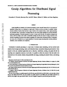
2.5.3 Simulation results In this subsection, the performance of the ZA–LMS and the RZA–LMS algorithms are compared with the standard LMS algorithm in terms of their MSD performance, based on a system identification scenario. System identification involves the following steps: experimental planning, the selection of a model structure, parameter estimation, and model validation [9]. Suppose we have an unknown plant ω 0 which is linear. x(i) is the available input signal at time instant i with size M × 1 and is applied simultaneously to the plant and the model. Then, d(i) and y(i) are employed to stand for the desired signal and the output of the adaptive 32


filter respectively. The output y(i) is obtained by y(i) = ω H (i)x(i),

(2.60)

where ω(i) is the estimate of the unknown plant generated by the adaptive filter. The error e(i) = d(i) − y(i) is used to adjust the adaptive filter. The task of the adaptive filtering algorithm is to keep the modeling error small [33]. The structure for the system identification is shown in Fig. 2.7. y(n) Adaptive Filter e(n)

System input

Unknown Plant

d(n)

System output

Observed Noise

Figure 2.7: System identification

The unknown plant ω 0 contains 20 coefficients and three scenarios are considered. In the first scenario, we set the 5th coefficient with value 1 and others to zero, forcing the system to have a sparsity level of 1/20. In the second scenario, all the odd coefficients are set to 1 while all the even coefficients remaining to be zero, i.e., a sparsity level of 10/20. In the third scenario, all the even coefficients are set with value -1 while all the odd coefficients are maintained to be 1, leaving a completely non–sparse system. The input signal and the observed noise are white Gaussian random sequences with variance of 1 and 10−3 , respectively. The parameters are set as µ = 0.05, ρ = 5 × 10−4 and ε = 10. Note that the same µ and ρ are used for the LMS, ZA–LMS and RZA–LMS algorithms. The average mean square deviation (MSD) is shown in Fig. 2.8, 2.9 and 2.10. It is clear that, from Fig. 2.8, when the system is very sparse, both ZA–LMS and RZA–LMS yield faster convergence rate and better steady–state performances than the LMS algorithm. The RZA–LMS algorithm achieves lower MSD than ZA–LMS. In the second scenario, as the number of non–zero coefficients increases to 10, the performance of ZA–LMS deteriorates while RZA–LMS maintains the best performance among the 33


three algorithm. In the third scenario, RZA–LMS still performs comparably with the standard LMS algorithm even though the system is now completely non–sparse.

5

LMS ZA−LMS RZA−LMS

0

−5

MSD (dB)

−10

−15

−20

−25

−30

−35 0

50

100

150

200

250 Time i

300

350

400

450

500

Figure 2.8: MSD comparison for scenario 1

2.6 Summary In this chapter, we have presented an overview of the theory relevant to this thesis and introduced the applications that are used to present the work in this thesis, including distributed estimation, spectrum estimation and smart grids. The topics of distributed signal processing, incremental and diffusion strategies, adaptive signal processing, compressive sensing and sparsity–aware techniques are then covered and discussed with an outline of previous work in these fields and important applications.

34


10


5 0

MSD (dB)

−5 −10 −15 −20 −25 −30 −35 0

50

100

150

200

250 Time i

300

350

400

450

500


15


10 5

MSD (dB)

0 −5 −10 −15 −20 −25 −30 0

50

100

150

200

250 Time i

300

350

400


35

450

500

Chapter 3 Distributed Conjugate Gradient Strategies for Distributed Estimation Over Sensor Networks Contents 3.1

Introduction . . . . . . . . . . . . . . . . . . . . . . . . . . . . . . . 36

3.2

System Models . . . . . . . . . . . . . . . . . . . . . . . . . . . . . . 38

3.3

Proposed Incremental Distributed CG–Based Algorithms . . . . . . 41

3.4

Proposed Diffusion Distributed CG–Based Algorithms . . . . . . . . 46

3.5

Preconditioner Design . . . . . . . . . . . . . . . . . . . . . . . . . . 48

3.6

Simulation Results . . . . . . . . . . . . . . . . . . . . . . . . . . . . 52

3.7

Summary . . . . . . . . . . . . . . . . . . . . . . . . . . . . . . . . . 58

3.1 Introduction In recent years, distributed processing has become popular in wireless networks. Distributed processing of information consists of collecting data at each node of a network of sensing devices spread over a geographical area, conveying information to the whole network and performing statistical inference in a distributed way [1, 47]. These techniques 36

CHAPTER 3. DISTRIBUTED CONJUGATE GRADIENT STRATEGIES FOR DISTRIBUTED ESTIMATION OVER SENSOR NETWORKS

exhibit several distinctive advantages such as flexibility, robustness to sensor failures and improved performance. In this context, for each specific node, a set of neighbor nodes collect their local information and transmit their estimates to the specific node. Then, each specific node combines the collected information together with its local estimate to generate an improved estimate. There are three main protocols for cooperation and exchange of information for distributed processing, incremental, diffusion and consensus strategies, and recent studies indicate that the diffusion strategy is the most effective one [5]. In the last few years, several algorithms have been developed and reported in the literature for distributed networks. Steepest-descent, least mean square (LMS) [1], recursive least squares (RLS) [48] and affine projection (AP) [16] solutions have been considered with incremental adaptive strategies over distributed networks [1], while LMS, AP and recursive least squares (RLS) algorithms have been reported using diffusion adaptive strategies [2, 18, 20, 49, 50]. Although the LMS–based algorithms have their own advantages, when compared with conjugate gradient (CG) algorithms, there are several disadvantages. First, for the LMS–based algorithms, the adaptation speed is often slow, especially for the conventional LMS algorithm. Second, with the increase of the adaptation speed, the system stability may decrease significantly [13]. Furthermore, the RLS–based algorithms usually are prone to numerical instability when implemented in hardware [9]. In order to develop distributed solutions with a more attractive tradeoff between performance and complexity, we focus on the development of distributed CG algorithms. To the best of our knowledge, CG–based algorithms have not been developed so far for distributed processing. The existing standard CG algorithm has a faster convergence rate than the LMS-type algorithms and a lower computational complexity than RLS–type algorithms, depending on the number of iterations that CG employs [6–8]. We consider variants of CG algorithms, including the conventional CG (CCG) and modified CG (MCG) algorithms [8, 51]. In this chapter, we propose distributed CG algorithms for both incremental and diffusion adaptive strategies. In particular, we develop distributed versions of the CCG algorithm and of the MCG algorithm for distributed estimation and spectrum estimation using wireless sensor networks. The design of preconditioners for CG algorithms, which have the ability to improve the performance of the CG algorithms is also presented in this chapter. These algorithms can be applied to civilian and defence applications, such

37


as parameter estimation in wireless sensor networks, biomedical engineering, cellular networks, battlefield information identification, movement estimation and detection and distributed spectrum estimation. In summary, the main contributions of this chapter are:

• We devise distributed CCG and MCG algorithms for incremental and diffusion strategies to perform distributed estimation tasks. • The design of preconditioners for CG algorithms, which have the ability to improve the performance of the proposed CG algorithms. • A simulation study of the proposed and existing distributed estimation algorithms with applications to distributed parameter estimation and spectrum estimation.

3.2 System Models In this section, we describe the system models of two applications of distributed signal processing, namely, parameter estimation and spectrum estimation. In these applications, we consider a wireless sensor network which employs distributed signal processing techniques to perform the desired tasks. We consider a set of N nodes, distributed over a given geographical area. The nodes are connected and form a network, which is assumed to be partially connected because nodes can exchange information only with neighbors determined by the connectivity topology. We call a network with this property a partially connected network whereas a fully connected network means that data broadcast by a node can be captured by all other nodes in the network in one hop [19].

3.2.1 Distributed Parameter Estimation For distributed parameter estimation, we focus on the processing of estimating an unknown vector ω 0 with size M × 1. The desired signal of each node at time instant i

38


is dk (i) = ω H 0 xk (i) + nk (i), i = 1, 2, . . . , I,

(3.1)

where xk (i) is the M × 1 input signal vector, nk (i) is the Gaussian noise at each node 2 with zero mean and variance σn,k . At the same time, the output of the adaptive algorithm

for each node is given by yk (i) = ω H k (i)xk (i), i = 1, 2, . . . , I,

(3.2)

where ω k (i) is the local estimate of ω 0 for each node at time instant i. To compute an estimate of the unknown vector, we need to solve a problem expressed in the form of a minimization of the cost function in the distributed form for each node k: 2 ( ) Jk ω k (i) = E dk (i) − ω H (i)x (i) k k

(3.3)

and the global network cost function could be described as N 2 ) ∑ E dk (i) − ω H J ω k (i) = k (i)xk (i) .

(

(3.4)

k=1

The optimum solution for the cost function (3.3) is the Wiener solution which is given by ω 0 = R−1 k (i)bk (i).

(3.5)

where the M × M autocorrelation matrix is given by Rk (i) = E[xk (i)xH k (i)] and bk (i) = E[xk (i)d∗k (i)] is an M × 1 cross–correlation matrix. In this chapter, we focus on incremental and diffusion CG–based algorithms to solve the equation and perform parameter estimation and spectrum estimation in a distributed fashion.

3.2.2 Distributed Spectrum Estimation In distributed spectrum estimation, we aim to estimate the spectrum of a transmitted signal s with N nodes using a wireless sensor network. Let Φs (f ) denote the power spectral density (PSD) of the signal s. The PSD can be represented as a linear combination of some B basis functions, as described by Φs (f ) =

B ∑

bm (f )ω0m = bT0 (f )ω 0 ,

m=1

39

(3.6)


where b0 (f ) = [b1 (f ), ..., bB (f )]T is the vector of basis functions evaluated at frequency f , ω 0 = [ω01 , ..., ω0B ] is a vector of weighting coefficients representing the power that transmits the signal s over each basis, and B is the number of basis functions. For B sufficiently large, the basis expansion in (3.6) can well approximate the transmitted spectrum. Possible choices for the set of basis {bm (f )}Bm=1 include [22–24]: rectangular functions, raised cosines, Gaussian bells and Splines. Let Hk (f, i) be the channel transfer function between a transmit node conveying the signal s and receive node k at time instant i, the PSD of the received signal observed by node k can be expressed as Ik (f, i) = |Hk (f, i)|2 Φs (f ) + vk2 =

B ∑

|Hk (f, i)|2 bm (f )ω0m + vk2

m=1

= bTk,i (f )ω 0 + vk2

(3.7)

where bTk,i (f ) = [|Hk (f, i)|2 bm (f )]Bm=1 and vk2 is the receiver noise power at node k. At every time instant i, every node k observes measurements of the noisy version of the true PSD Ik (f, i) described by (3.7) over Nc frequency samples fj = fmin : (fmax − fmin )/Nc : fmax , for j = 1, ..., Nc , according to the model: djk (i) = bTk,i (fj )ω 0 + vk2 + njk (i).

(3.8)

2 The term njk (i) denotes sampling noise and have zero mean and variance σn,j . The re2 ceiver noise power vn,k can be estimated with high accuracy in a preliminary step using,

e.g., an energy estimator over an idle band, and then subtracted from (3.8) [25, 26]. Thus, collecting measurements over Nc contiguous channels, we obtain a linear model given by dk (i) = B k (i)ω 0 + nk (i),

(3.9)

Nc ×B T c c where B k (i) = [bTk,i (fj )]N , with Nc > B, and nk (i) = [n1k (i), ...nN j=1 ∈ R k (i)] . At

this point, we can generate the cost function for node k as: 2 Jωk (i) (ω k (i)) = E dk (i) − B k (i)ω k (i)

(3.10)

and the global network cost function could be described as N 2 ( ) ∑ E dk (i) − B k (i)ω . Jω ω = k=1

40

(3.11)


3.3 Proposed Incremental Distributed CG–Based Algorithms In this section, we propose two CG–based algorithms which are based on the CCG [8] and MCG [52] algorithms with incremental distributed solution for distributed parameter estimation and spectrum estimation over wireless sensor networks.

3.3.1 Incremental Distributed CG–Based Solutions In the incremental distributed strategy, each node is only allowed to communicate with its direct neighbor at each time instant. To describe the whole process, we define a cycle where each node in this network could only access its immediate neighbor in this cycle [1]. The quantity ψ k (i) is defined as a local estimate of the unknown vector ω 0 at time instant i. As a result, we assume that node k has access to an estimate of ω 0 at its immediate neighbor node k − 1 which is ψ k−1 (i) in the defined cycle. Fig.3.1 illustrates this processing. In the following, we introduce two kinds of incremental distributed CG–

Node k-1 ψk−1(i) Node 1

Node k

ψk−1(i)

dk (i), xk (i)

Incremental Distributed CG–Based Algorithm

ψk (i) ψk (i), pass to node k+1 Node N

Node k+1 Figure 3.1: Incremental distributed CG–based network processing

based algorithms, which are the incremental distributed CCG (IDCCG) algorithm and the incremental distributed MCG (IDMCG) algorithm.

41


Proposed IDCCG Algorithm

Based on the main steps of CG algorithm which are described in Table. 2.4, we introduce the main steps of the proposed IDCCG algorithm. In the IDCCG algorithm, the iteration procedure is introduced. At the jth iteration of time instant i, the step size αkj (i) for updating the local estimate at node k is defined as: (

αkj (i)

)H j−1 g j−1 g k (i) k (i) = ( j−1 )H , pk (i) Rk (i)pkj−1 (i)

(3.12)

where pjk (i) is the search direction and defined as pjk (i) = g jk (i) + βkj (i)pkj−1 (i).

(3.13)

In (3.13), the coefficient βkj (i) is calculated by the Gram–Schmidt orthogonalization procedure [7] for the conjugacy: (

βkj (i)

)H g jk (i) g jk (i) = ( j−1 )H j−1 . g k (i) g k (i)

(3.14)

g jk (i) is the residual, which is obtained as j j−1 g jk (i) = g j−1 k (i) − αk (i)Rk (i)pk (i).

(3.15)

The initial search direction is equal to the initial residual, which is given by p0k (i) = g 0k (i) = bk (i) − Rk (i)ψ 0k (i). Then, the local estimate is updated as j j−1 ψ jk (i) = ψ j−1 k (i) + αk (i)pk (i).

(3.16)

There are two ways to compute the correlation and cross–correlation matrices which are the ’finite sliding data window’ and the ’exponentially decaying data window’ [8]. In this chapter, we focus on the ’exponentially decaying data window’. The recursions are given by: Rk (i) = λf Rk (i − 1) + xk (i)xH k (i)

(3.17)

bk (i) = λf bk (i − 1) + d∗k (i)xk (i)

(3.18)

and

where λf is the forgetting factor. The IDCCD algorithm is summarized in Table 3.1 42


Table 3.1: IDCCG Algorithm Initialization:

Complexity

Complexity

Multiplications

Additions

Rk (i) = λf Rk (i − 1) + xk (i)xH k (i)

2M 2

M2

bk (i) = λf bk (i − 1) + d∗k (i)xk (i)

2M

M

ω(0) = 0 For each time instant i = 1, 2, . . . , I ψ 01 (i) = ω(i − 1) For each node k = 1, 2, . . . , N

p0k (i)

=

g 0k (i)

= bk (i) −

Rk (i)ψ 0k (i)

For iterations j = 1, 2, . . . , J ( j−1 )H j−1 g (i) g (i) j αk (i) = ( j−1k )H k j−1

M

2

2M 2

M 2 + 2M + 1

M2 + M − 2

j j−1 ψ jk (i) = ψ j−1 k (i) + αk (i)pk (i)

M

M

j j−1 g jk (i) = g j−1 k (i) − αk (i)Rk (i)pk (i) ( j )H j g (i) g k (i) βkj (i) = ( j−1k )H j−1

M

M

M +1

M −1

M

M

pk

gk

(i)

(i)

Rk (i)pk

gk

(i)

(i)

pjk (i) = g jk (i) + βkj (i)pj−1 k (i) End When k < N ψ 0k+1 (i) = ψ Jk (i) End ω(i) = ψ JN (i) End

43


Proposed IDMCG Algorithm

The idea of the IDMCG algorithm comes from the existing MCG algorithm. For the IDMCG solution, a recursive formulation for the residual vector is employed, which can be found by using (3.12), (3.17) and (3.18) [8, 51], resulting in g k (i) = bk (i) − Rk (i)ψ k (i) = λf g k (i − 1) − αk (i)Rk (i)pk (i − 1) + xk (i)[dk (i) −

ψH k−1 (i)xk (i)].

(3.19)

Premultiplying (3.19) by pH k (i − 1) gives H H pH k (i − 1)g k (i) = λf pk (i − 1)g k (i − 1) − αk (i)pk (i − 1)Rk (i)pk (i − 1) H + pH k (i − 1)xk (i)[dk (i) − ψ k−1 (i)xk (i)].

(3.20)

Taking the expectation of both sides and considering pk (i − 1) uncorrelated with xk (i), dk (i) and ψ k−1 (i) yields H H E[pH k (i − 1)g k (i)] ≈ λf E[pk (i − 1) g k−1 (i)] − E[αk (i)]E[pk (i − 1)Rk (i)pk (i − 1)] [ ] H + E[pH k (i − 1)]E xk (i)[dk (i) − ω k−1 (i)xk (i)] .

(3.21) Assuming that the algorithm converges, the last term of (3.21) can be neglected and we obtain [8]: E[αk (i)] =

H E[pH k (i − 1)g k (i)] − λf E[pk (i − 1)g k (i − 1)] E[pH k (i − 1)Rk (i)pk (i − 1)]

(3.22)

and the E[αk (i)] should satisfied the following equation [8]: (λf − 0.5)

E[pH E[pH k (i − 1)g k (i − 1)] k (i − 1)g k (i − 1)] ≤ E[α (i)] ≤ k H H E[pk (i − 1)Rk (i)pk (i − 1)] E[pk (i − 1)Rk (i)pk (i − 1)] (3.23)

The inequalities in (3.23) are satisfied if we define [8]: αk (i) = η

pH k (i − 1)g k (i − 1) , pH k (i − 1)Rk (i)pk (i − 1)

(3.24)

where (λf − 0.5) ≤ η ≤ λf . The direction vector pk (i) for the IDMCG algorithm is defined by pk (i) = g k (i) + βk (i)pk (i − 1).

44

(3.25)


Table 3.2: IDMCG Algorithm Initialization: ω(0) = 0

Complexity

Complexity

Multiplications

Additions

2M 2

M2

M 2 + 2M + 1

M2 + M − 2

M

M

4M

3M

2M + 1

3M − 2

M

M

For each node k = 1, 2, . . . , N bk (1) = d∗k (1)xk (1) pk (0) = g k (0) = bk (1) End For each time instant i = 1, 2, . . . , I ψ 0 (i) = ω(i − 1) For each node k = 1, 2, . . . , N Rk (i) = λf Rk (i − 1) + xk (i)xH k (i) pH (i−1)g (i−1) k (i−1) k

k k αk (i) = η pH (i−1)R k (i)p

where (λf − 0.5) ≤ η ≤ λf ψ k (i) = ψ k−1 (i) + αk (i)pk (i − 1) g k (i) = λf g k (i − 1) − αk (i)Rk (i)pk (i − 1) +xk (i)[dk (i) − ψ H (i)xk (i)] ( )H k−1 βk (i) =

g k (i)−g k (i−1)

g k (i)

gH k (i−1)g k (i−1)

pk (i) = g k (i) + βk (i)pk (i − 1) End ω(i) = ψ N (i) End

For the IDMCG algorithm, for the computation of βk (i), the Polak–Ribiere method [8], which is given by

(

)H g k (i) − g k (i − 1) g k (i) βk (i) = gH k (i − 1)g k (i − 1)

(3.26)

should be used for improved performance, according to [53, 54]. In the comparison of the IDCCG algorithm with the IDMCG algorithm, the difference between these two strategies is that IDCCG needs to run J iterations while IDMCG only needs one iteration. The details of the IDMCG solution are shown in Table 3.2.

45


Table 3.3: Computational Complexity of Different Incremental Algorithms per Node Algorithm

Additions

Multiplications

IDCCG

2M 2 + M

3M 2 + 2M

+J(M 2 + 5M − 4)

J(M 2 + 6M + 2)

IDMCG

2M 2 + 9M − 4

3M 2 + 10M + 2

Incremental LMS [1]

4M − 1

3M + 1

Incremental RLS [1]

4M 2 + 12M + 1

4M 2 + 12M − 1

3.3.2 Computational Complexity To analyze the proposed incremental distributed CG algorithms, we detail the computational complexity in terms of arithmetic operations. Additions and multiplications are used to measure the complexity and are listed in Table 3.3. The parameter M is the length of the unknown vector ω 0 that needs to be estimated. Detailed computational complexity of each step for the proposed incremental distributed CG algorithms are shown in Table 3.1 and 3.2. When compare the IDMCG and IDCCG algorithms with the RLS–type algorithm, we can see that the complexity of IDMCG is lower than the RLS algorithm, while the complexity of the IDCCG solution depends on the number of iterations J.

3.4 Proposed Diffusion Distributed CG–Based Algorithms In this section, we detail the proposed diffusion distributed CCG (DDCCG) and diffusion distributed MCG (DDMCG) algorithms for distributed parameter estimation and spectrum estimation using wireless sensor networks.

46


3.4.1 Diffusion Distributed CG–Based Algorithms In the derivation of diffusion distributed CG–based strategy, we consider a network structure where each node from the same neighborhood could exchange information with each other at every time instant. For each node in the network, the CTA scheme [17] is employed. Each node can collect information from all its neighbors and itself, and then convey all the information to its local adaptive algorithm and update the estimate of the weight vector through our algorithms. Specifically, at any time instant i, we define that node k has access to a set of estimates {ω l (i − 1)}l∈Nk from its neighbors, where Nk denotes the set of neighbor nodes of node k including node k itself. Then, these local estimates are combined at node k as ψ k (i) =

∑

ckl ω l (i − 1)

(3.27)

l∈Nk

where ckl is calculated through the Metropolis rule in (2.16) due to its simplicity and good performance [55]. For the proposed diffusion distributed CG–based algorithms, the whole processing is shown in Fig. 3.2.

Node k-1 ωk−1(i − 1) Node k Node 1

dk (i), xk (i)

ψk (i)

Diffusion Distributed CG–Based Algorithm

ω1(i − 1) ωk+1(i − 1)

Node N

ωk (i) Node k+1 Figure 3.2: Diffusion Distributed CG–Based Network Processing

Proposed DDCCG Algorithm

For the DDCCG algorithm, (3.27) is employed to combine the estimates ω l (i − 1), l ∈ Nk from node k’s neighbor nodes and then the estimate at node k is updated as follows: j j−1 ω jk (i) = ω j−1 k (i) + αk (i)pk (i),

47

(3.28)


where ω 0k (i) = ψ k (i). The rest of the derivation is similar to the IDCCG solution and the pseudo–code is detailed in Table 3.4.

Proposed DDMCG Algorithm

For the DDMCG algorithm, the iteration j is removed and the estimate at node k is updated as: ω k (i) = ψ k (i) + αk (i)pk (i),

(3.29)

The complete DDMCG algorithm is described in Table 3.5.

3.4.2 Computational Complexity The proposed diffusion distributed CG–based algorithms are analysed in terms of computational complexity, where additions and multiplications are measured. The details are listed in Table 3.6. Similarly to the incremental distributed CG–based algorithms, it is clear that the complexity of the DDCCG solution depends on the iteration number J and both DDCCG and DDMCG solutions depend on the number of neighbor nodes |Nk | of node k. The parameter M is the length of the unknown vector ω 0 that needs to be estimated.

3.5 Preconditioner Design Preconditioning is an important technique which can be used to improve the performance of CG algorithms [56–59]. The idea behind preconditioning is to employ the CG algorithms on an equivalent system or in a transform–domain. Thus, instead of solving ˜ which is modified with the aim of ob˜ω ˜ = b, Rω = b we solve a related problem R taining better convergence and steady state performance. The relationships between these two equations are given by ˜ = T RT H , R

48

(3.30)


Table 3.4: DDCCG Algorithm Initialization: ω k (0) = 0, k = 1, 2, . . . , N For each time instant i = 1, 2, . . . , I For each node k = 1, 2, . . . , N (Combination Step) ∑ ψ k (i) = l∈Nk ckl ω l (i − 1) End For each node k = 1, 2, . . . , N (Adaptation Step) Rk (i) = λf Rk (i − 1) + xk (i)xH k (i) bk (i) = λf bk (i − 1) + d∗k (i)xk (i) ω 0k (i) = ψ k (i) p0k (i) = g 0k (i) = bk (i) − Rk (i)ω 0k (i) For iterations j = 1, 2, . . . , J ( j−1 )H j−1 g (i) g (i) j αk (i) = ( j−1k )H k j−1 pk

(i)

Rk (i)pk

(i)

j j−1 ω jk (i) = ω j−1 k (i) + αk (i)pk (i) j j−1 g jk (i) = g j−1 k (i) − αk (i)Rk (i)pk (i)

(

βkj (i) pjk (i)

=( =

g jk (i)

g j−1 (i) k

g jk (i)

)H j g k (i) )H j−1

+

End ω k (i) = ω Jk (i) End End

49

gk

(i)

βkj (i)pkj−1 (i)


Table 3.5: DDMCG Algorithm Initialization: ω k (0) = 0, k = 1, 2, . . . , N For each node k = 1, 2, . . . , N bk (1) = d∗k (1)xk (1) pk (0) = g k (0) = bk (1) End For each time instant i = 1, 2, . . . , I For each node k = 1, 2, . . . , N (Combination Step) ∑ ψ k (i) = l∈Nk ckl ω l (i − 1) End For each node k = 1, 2, . . . , N (Adaptation Step) Rk (i) = λf Rk (i − 1) + xk (i)xH k (i) bk (i) = λf bk (i − 1) + d∗k (i)xk (i) pH (i−1)g (i−1) k (i−1) k

k k αk (i) = η pH (i−1)R k (i)p

where (λf − 0.5) ≤ η ≤ λf ω k (i) = ψ k (i) + αk (i)pk (i − 1) g k (i) = λf g k (i − 1) − αk (i)Rk (i)pk (i − 1) + xk (i)[dk (i) − ψ H k−1 (i)xk (i)] ( )H g (i)−g k (i−1) g k (i) βk (i) = k gH (i−1)g (i−1) k

k

pk (i) = g k (i) + βk (i)pk (i − 1) End End Table 3.6: Computational Complexity Of Different Diffusion Algorithms per Node Algorithm

Additions

Multiplications

DDCCG

2M 2 + M

3M 2 + 2M

+J(M 2 + 5M

+J(M 2 + 6M

+|Nk |M − 4)

+|Nk |M + 2)

2M 2 + 9M − 4

3M 2 + 10M + 2

+|Nk |M

+|Nk |M

Diffusion LMS [17]

4M − 1 + |Nk |M

3M + 1 + |Nk |M

Diffusion RLS [20]

4M 2 + 16M + 1 + |Nk |M

4M 2 + 12M − 1 + |Nk |M

DDMCG

50


˜ = Tω ω

(3.31)

˜ = T b, b

(3.32)

and

where the M × M matrix T is called a preconditioner. We design the matrix T as an arbitrary unitary matrix that has the following property [10] T T H = T H T = I.

(3.33)

Two kinds of unitary transformations are considered to build the preconditioner T , which are discrete Fourier transform (DFT) and discrete cosine transform (DCT) [10]. The motivation behind employing these two matrix is they have useful de–correlation properties and often reduce the eigenvalue spread of the auto–correlation matrix of the input signal [10]. For the DFT scheme, we employ the following expression j2πmv 1 [T DF T ]vm , √ e− M , v, m = 0, 1, 2, . . . , M − 1, M

(3.34)

where v indicates the row index and m the column index. M is the length of the unknown parameter ω 0 . The matrix form of T DF T is illustrated as  1 1 1  j2π j4π 1 e− M e− M  1  j4π j8π T DF T = √  1 e− M e− M  M . .. ..  .. . .  j4(M −1)π j2(M −1)π e− M 1 e− M



···

1

···

e−

j2(M −1)π M

··· .. .

e−

j4(M −1)π M

· · · e−

.. . j2(M −1)2 π M

        

For the DCT scheme, the preconditioner T is defined as ) ( v(2m + 1)π [T DCT ]vm , δ(v) cos , v, m = 0, 1, 2, . . . , M − 1, 2M where 1 δ(0) = √ and δ(v) = M

51

√

2 for v ̸= 0 M

(3.35)

(3.36)

(3.37)


and the matrix form of T DCT is illustrated as  1 1 1  √ √ 1 3π 5π 2 cos( 2M ) 2 cos( 2M )  √ √ 1  6π T DCT = √  1 2 cos( 2M ) 2 cos( 10π ) 2M M . .. ..  .. . .  √ √ −1)π −1)π 1 2 cos( 3(M2M ) 2 cos( 5(M2M )

···

 1

     ···   ..  .  √ (2M −1)(M −1)π ··· 2 cos( ) 2M (3.38) ···

√ −1)π 2 cos( (2M2M ) √ −1)π 2 cos( 2(2M ) 2M .. .

Then, for the DCT scheme, we choose T = T H DCT . It should be noticed that the scaling factor

√1 M

is added in the expression for the T DF T in order to result in a unitary

H transformation since then T DF T satisfies T DF T T H DF T = T DF T T DF T = I [10].

The optimal selection of the preconditioner is the Karhunen–Lo`eve transform (KLT) [10]. However, using the KLT is not practical since it requires knowledge of the auto– correlation matrix R of the input signal and this information is generally lacking in implementations.

3.6 Simulation Results In this section, we investigate the performance of the proposed incremental and diffusion distributed CG–based algorithms in two scenarios: distributed estimation and distributed spectrum estimation in wireless sensor networks.

3.6.1 Distributed Estimation in Wireless Sensor Networks In this subsection, we compare the proposed incremental and diffusion distributed CG– based algorithms with LMS [1, 17] and RLS [1, 20] algorithms, based on the MSE and MSD performance metrics. For each comparison, the number of time instants is set to 1000, and we assume there are 20 nodes in the network. The length of the unknown parameter vector ω 0 is 10, the variances for the input signal and the noise are 1 and 0.001, respectively. In addition, the noise samples are modeled as circular Gaussian noise with zero mean. 52


Performance of Proposed Incremental Distributed CG–Based Algorithms

First, we define the parameters of the performance test for each algorithm and the network. The step size µ for the LMS algorithm [1] is set to 0.2, the forgetting factor λ for the RLS [1] algorithm is set to 0.998. The λf for IDCCG and IDMCG are both set to 0.998. For IDMCG, the η is equal to 0.55. The iteration number J for IDCCG is set to 5. We choose the DCT matrix as the preconditioner.

0

Incremental LMS[1] Incremental RLS[1] IDCCG IDMCG Preconditioned IDCCG Preconditioned IDMCG

−5

−10

MSD(dB)

−15

−20

−25

−30

−35

−40

−45 0

100

200

300

400

500 600 Time instant

700

800

900

1000

Figure 3.3: MSD performance comparison for the incremental distributed strategies

The MSD and MSE performances of each algorithm is shown in Fig. 3.3 and 3.4 respectively. We can verify that, the IDMCG and IDCCG algorithm performs better than incremental LMS, while IDMCG is close to the RLS algorithm. With the preconditioning strategy, the performance of the IDCCG and IDMCG is further improved. The reason why the proposed IDMCG algorithm has a better performance than IDCCG is because IDMCG employs the negative gradient vector g k with a recursive expression and the βk is computed using the Polak–Ribiere approach, which results in more accurate estimates. Comparing with the IDCCG algorithm, the IDMCG is a non–reset and low complexity algorithm with one iteration per time instant. Since the frequency which the algorithm resets influences the performance, the IDMCG algorithm introduces the non–reset method 53


5

Incremental LMS[1] Incremental RLS[1] IDCCG IDMCG Preconditioned IDCCG Preconditioned IDMCG

0

MSE(dB)

−5

−10

−15

−20

−25

−30 0

100

200

300

400

500 600 Time instant

700

800

900

1000

Figure 3.4: MSE performance comparison for the incremental distributed strategies

together with the Polak– Ribiere approach which are used to improve the performance [8]. In detail, according to (3.26), when g k (i) ≈ g k (i − 1), βk (i) ≈ 0. This will lead to pk (i) ≈ g k (i), which means the algorithm is reset.

Performance of Proposed Diffusion Distributed CG–Based Algorithms

The parameters of the performance test for each algorithm and the network are defined as follows: the step size µ for the LMS [17] algorithm is set to 0.2, the forgetting factor λ for the RLS [20] algorithm is set to 0.998. The λf for DDCCG and DDMCG are both 0.998. The η is equal to 0.45 for DDMCG. The iteration number J for DDCCG is set to 5. We choose the DCT matrix as the preconditioner. For the diffusion strategy, the combining coefficients ckl are calculated following the Metropolis rule. Fig. 3.5 shows the network structure. The results are illustrated in Fig. 3.6 and 3.7. We can see that, the proposed DDMCG and DDCCG still have a better performance than the LMS algorithm and DDMCG is closer to the RLS’s performance. The performance of the DDCCG and DDMCG can still benefit from the preconditioning 54


strategy.

20

14

12 11

18

16

10 4

14

18

20 12

10

9

15

7

8

19

8

6

13

4

3

6 17

2

16 0

0

2

4

6

2

1 8

10

12

5 14

16

18

20

Figure 3.5: Network structure

10

Diffusion LMS[17] Diffusion RLS[20] DDCCG DDMCG Preconditioned DDCCG Preconditioned DDMCG

0

MSD(dB)

−10

−20

−30

−40

−50 0

100

200

300

400 500 600 Time instant

700

800

900

1000

Figure 3.6: MSD performance comparison for the diffusion distributed strategies

55


5

Diffusion LMS[17] Diffusion RLS[20] DDCCG DDMCG Preconditioned DDCCG Preconditioned DDMCG

0

MSE(dB)

−5

−10

−15

−20

−25

−30 0

100

200

300

400 500 600 Time instant

700

800

900

1000

Figure 3.7: MSE performance comparison for the diffusion distributed strategies

3.6.2 Distributed Spectrum Estimation In this simulation, we consider a network composed of N = 20 nodes estimating the unknown spectrum ω 0 , as illustrated in Fig. 3.5. The nodes scan Nc = 100 frequencies over the frequency axis, which is normalized between 0 and 1, and use B = 50 non– overlapping rectangular basis functions to model the expansion of the spectrum [25]. The basis functions have amplitude equal to one. We assume that the unknown spectrum ω 0 is transmitted over 8 basis functions, thus leading to a sparsity ratio equal to 8/50. The power transmitted over each basis function is set equal to 0.7. The variance for the observation noise is 0.01. For distributed estimation, we employ the DDMCG and the DDCCG algorithms, together with the preconditioned DDMCG algorithm to solve the cost function (3.11). The λf for DDCCG and DDMCG are both 0.99. The ηf is equal to 0.3 for DDMCG. The iteration number J for DDCCG is set to 5. The DCT matrix is employed as the preconditioner. We compare the proposed DDCCG and DDMCG algorithms with the sparse ATC diffusion algorithm [25], diffusion LMS algorithm [17] and diffusion RLS algorithm [20]. 56


The step–sizes for the sparse ATC diffusion algorithm and diffusion LMS algorithm are set equal to 0.2, while for the sparse ATC diffusion algorithm, γ is set to 2.2 × 10−3 and β is set to 50. The forgetting factor λ for the diffusion RLS algorithm is set to 0.998.

10

DDMCG Preconditioned DDMCG Diffusion LMS[17] Sparse ATC diffusion[25] DDCCG Diffusion RLS[20]

5

MSD (dB)

0

−5

−10

−15

−20

−25 0

20

40

60

80 100 Time instant

120

140

160

180

Figure 3.8: Performance comparison for the distributed spectrum estimation

We illustrate the result of distributed spectrum estimation carried out by different algorithms in the term of the MSD comparison in Fig. 3.8. We also select the sparse ATC diffusion algorithm [25], diffusion LMS algorithm [17] and DDMCG to compare their performance in term of PSD in Fig. 3.9. The true transmitted spectrum is also reported in Fig. 3.9. From Fig. 3.8, the DDMCG still performs better than other algorithms and is close to the diffusion RLS algorithm. From Fig. 3.9, we can notice that all the algorithms are able to identify the spectrum, but it is also clear that the DDMCG algorithm is able to strongly reduce the effect of the spurious terms.

57


0

Diffusion LMS[17] Sparse ATC Diffusion[25] DDMCG True spectrum

−5

PSD (dB)

−10

−15

−20

−25

−30

0

0.1

0.2

0.3

0.4

0.5

0.6

0.7

0.8

0.9

1

Frequency Axis

Figure 3.9: Example of distributed spectrum estimation

3.7 Summary In this chapter, we have proposed distributed CG algorithms for both incremental and diffusion adaptive strategies. We have investigated the proposed algorithms in distributed estimation for wireless sensor networks and distributed spectrum estimation. The CG–based strategies have a lower computational complexity than RLS–type algorithms, depending on the number of iterations that CG employs and a faster convergence than the LMS algorithm. The preconditioning strategy is also introduced to further improve the performance of the proposed algorithms. Simulation results have illustrated the advantages of the proposed IDCCG/IDMCG and DDCCG/DDMCG algorithms in different applications.

58

Chapter 4 Adaptive Link Selection Algorithms for Distributed Diffusion Estimation Contents 4.1

Introduction . . . . . . . . . . . . . . . . . . . . . . . . . . . . . . . 59

4.2

System Model and Problem Statement . . . . . . . . . . . . . . . . . 62

4.3

Proposed Adaptive Link Selection Algorithms . . . . . . . . . . . . 64

4.4

Analysis of the proposed algorithms . . . . . . . . . . . . . . . . . . 72

4.5

Simulations . . . . . . . . . . . . . . . . . . . . . . . . . . . . . . . . 90

4.6

Summary . . . . . . . . . . . . . . . . . . . . . . . . . . . . . . . . . 100

4.1 Introduction Distributed signal processing algorithms have become a key approach for statistical inference in wireless networks and applications such as wireless sensor networks and smart grids [1–4]. It is well known that distributed processing techniques deal with the extraction of information from data collected at nodes that are distributed over a geographic area [1]. In this context, for each specific node, a set of neighbor nodes collect their local information and transmit the estimates to a specific node. Then, each specific node combines the collected information together with its local estimate to generate an improved 59

CHAPTER 4. ADAPTIVE LINK SELECTION ALGORITHMS FOR DISTRIBUTED DIFFUSION ESTIMATION

estimate.

4.1.1 Prior and Related Work Several works in the literature have proposed strategies for distributed processing which include incremental [1, 60–62], diffusion [2, 17], sparsity–aware [3, 63] and consensus– based strategies [18]. With the incremental strategy, the processing follows a Hamiltonian cycle, i.e., the information flows through these nodes in one direction, which means each node passes the information to its adjacent node in a uniform direction. However, in order to determine an optimum cyclic path that covers all nodes (considering the noise, interference, path loss and channels between neighbor nodes), this method needs to solve an NP–hard problem. In addition, when any of the nodes fails, data communication through the cycle is interrupted and the distributed processing breaks down [1]. In distributed diffusion strategies [2, 63], the neighbors for each node are fixed and the combining coefficients are calculated after the network topology is deployed and starts its operation. One potential risk of this approach is that the estimation procedure may be affected by poorly performing links. More specifically, the fixed neighbors and the pre– calculated combining coefficients may not provide an optimized estimation performance for each specified node because there are links that are more severely affected by noise or fading. Moreover, when the number of neighbor nodes is large, each node requires a large bandwidth and transmit power. Prior work on topology design and adjustment techniques includes the studies in [64, 65] and [66], which are not dynamic in the sense that they cannot track changes in the network and mitigate the effects of poor links.

4.1.2 Contributions The adaptive link selection algorithms for distributed estimation problems are proposed and studied in this chapter. Specifically, we develop adaptive link selection algorithms that can exploit the knowledge of poor links by selecting a subset of data from neighbor nodes. The first approach consists of exhaustive search–based LMS/RLS link selection (ES–LMS/ES–RLS) algorithms, whereas the second technique is based on sparsity– 60


inspired LMS/RLS link selection (SI–LMS/SI–RLS) algorithms. With both approaches, distributed processing can be divided into two steps. The first step is called the adaptation step, in which each node employs LMS or RLS to perform the adaptation through its local information. Following the adaptation step, each node will combine its collected estimates from its neighbors and local estimate, through the proposed adaptive link selection algorithms. The proposed algorithms result in improved estimation performance in terms of the mean–square error (MSE) associated with the estimates. In contrast to previously reported techniques, a key feature of the proposed algorithms is that the combination step involves only a subset of the data associated with the best performing links. In the ES–LMS and ES–RLS algorithms, we consider all possible combinations for each node with its neighbors and choose the combination associated with the smallest MSE value. In the SI–LMS and SI–RLS algorithms, we incorporate a reweighted zero attraction (RZA) strategy into the adaptive link selection algorithms. The RZA approach is often employed in applications dealing with sparse systems in such a way that it shrinks the small values in the parameter vector to zero, which results in better convergence and steady–state performance. Unlike prior work with sparsity–aware algorithms [3, 13, 67, 68], the proposed SI–LMS and SI–RLS algorithms exploit the possible sparsity of the MSE values associated with each of the links in a different way. In contrast to existing methods that shrink the signal samples to zero, SI–LMS and SI–RLS shrink to zero the links that have poor performance or high MSE values. By using the SI–LMS and SI– RLS algorithms, data associated with unsatisfactory performance will be discarded, which means the effective network topology used in the estimation procedure will change as well. Although the physical topology is not changed by the proposed algorithms, the choice of the data coming from the neighbor nodes for each node is dynamic, leads to the change of combination weights and results in improved performance. We also remark that the topology could be altered with the aid of the proposed algorithms and a feedback channel which could inform the nodes whether they should be switched off or not. The proposed algorithms are considered for wireless sensor networks and also as a tool for distributed state estimation that could be used in smart grids. In summary, the main contributions of this chapter are:

• We present adaptive link selection algorithms for distributed estimation that are able 61


to achieve significantly better performance than existing algorithms. • We devise distributed LMS and RLS algorithms with link selection capabilities to perform distributed estimation. • We analyze the MSE convergence and tracking performance of the proposed algorithms and their computational complexities and we derive analytical formulas to predict their MSE performance. • A simulation study of the proposed and existing distributed estimation algorithms is conducted along with applications in wireless sensor networks and smart grids.

4.2 System Model and Problem Statement

k

Nk Figure 4.1: Network topology with N nodes

We consider a set of N nodes, which have limited processing capabilities, distributed over a given geographical area as depicted in Fig. 4.1. The nodes are connected and form a network, which is assumed to be partially connected because nodes can exchange information only with neighbors determined by the connectivity topology. We call a network with this property a partially connected network whereas a fully connected network means that data broadcast by a node can be captured by all other nodes in the network in one hop [19]. We can think of this network as a wireless network, but our analysis also applies to wired networks such as power grids. In our work, in order to perform link selection strategies, we assume that each node has at least two neighbors. 62


The aim of the network is to estimate an unknown parameter vector ω 0 , which has length M . At every time instant i, each node k takes a scalar measurement dk (i) according to dk (i) = ω H 0 xk (i) + nk (i), i = 1, 2, . . . , I,

(4.1)

where xk (i) is the M × 1 random regression input signal vector and nk (i) denotes the 2 Gaussian noise at each node with zero mean and variance σn,k . This linear model is able

to capture or approximate well many input-output relations for estimation purposes [9] and we assume I > M . To compute an estimate of ω0 in a distributed fashion, we need each node to minimize the MSE cost function [2] 2 ( ) , Jk ω k (i) = E dk (i) − ω H (i)x (i) k k

(4.2)

where E denotes expectation and ω k (i) is the estimated vector generated by node k at time instant i. Equation (4.3) is also the definition of the MSE and the global network cost function could be described as J(ω) =

N ∑

E|dk (i) − ω H xk (i)|2 .

(4.3)

k=1

To solve this problem, diffusion strategies have been proposed in [2, 17] and [16]. In these strategies, the estimate for each node is generated through a fixed combination strategy given by ω k (i) =

∑

ckl ψ l (i),

(4.4)

l∈Nk

where Nk denotes the set of neighbors of node k including node k itself, ckl ≥ 0 is the combining coefficient and ψ l (i) is the local estimate generated by node l through its local information. There are many ways to calculate the combining coefficient ckl which include the Hastings [55], the Metropolis [30], the Laplacian [31] and the nearest neighbor [32] rules. In this work, due to its simplicity and good performance we adopt the Metropolis rule [30] given by (2.16). The set of coefficients ckl should satisfy [2] ∑

ckl = 1.

l∈Nk ∀k

63

(4.5)


For the combination strategy mentioned in (4.4), the choice of neighbors for each node is fixed, which results in some problems and limitations, namely:

• Some nodes may face high levels of noise or interference, which may lead to inaccurate estimates. • When the number of neighbors for each node is high, large communication bandwidth and high transmit power are required. • Some nodes may shut down or collapse due to network problems. As a result, local estimates to their neighbors may be affected.

Under such circumstances, a performance degradation is likely to occur when the network cannot discard the contribution of poorly performing links and their associated data in the estimation procedure. In the next section, the proposed adaptive link selection algorithms are presented, which equip a network with the ability to improve the estimation procedure. In the proposed scheme, each node is able to dynamically select the data coming from its neighbors in order to optimize the performance of distributed estimation techniques.

4.3 Proposed Adaptive Link Selection Algorithms In this section, we present the proposed adaptive link selection algorithms. The goal of the proposed algorithms is to optimize the distributed estimation and improve the performance of the network by dynamically changing the topology. These algorithmic strategies give the nodes the ability to choose their neighbors based on their MSE performance. We develop two categories of adaptive link selection algorithms; the first one is based on an exhaustive search, while the second is based on a sparsity–inspired relaxation. The details will be illustrated in the following subsections.

64


4.3.1 Exhaustive Search–Based LMS/RLS Link Selection The proposed ES–LMS and ES–RLS algorithms employ an exhaustive search to select the links that yield the best performance in terms of MSE. First, we describe how we define the adaptation step for these two strategies. In the ES–LMS algorithm, we employ the adaptation strategy given by ]∗ [ , (i)x (i) ψ k (i) = ω k (i) + µk xk (i) dk (i) − ω H k k

(4.6)

where µk is the step size for each node. In the ES–RLS algorithm, we employ the following steps for the adaptation: −1 −1 Φ−1 k (i) = λ Φk (i − 1) −1 H λ−2 Φ−1 k (i − 1)xk (i)xk (i)Φk (i − 1) , − −1 1 + λ−1 xH k (i)Φk (i − 1)xk (i)

(4.7)

where λ is the forgetting factor. Then, we let P k (i) = Φ−1 k (i) and

(4.8)

λ−1 P k (i)xk (i) . 1 + λ−1 xH k (i)P k (i)xk (i) [ ]∗ ψ k (i) = ω k (i) + k(i) dk (i) − ω H k (i)xk (i) ,

(4.10)

P k (i + 1) = λ−1 P k (i) − λ−1 kk (i)xH k (i)P k (i).

(4.11)

kk (i) =

(4.9)

Following the adaptation step, we introduce the combination step for both ES–LMS and ES–RLS algorithms, based on an exhaustive search strategy. At first, we introduce a tentative set Ωk using a combinatorial approach described by Ωk ∈ 2|Nk | \∅,

(4.12)

where the set Ωk is a nonempty set with 2|Nk | elements. After the tentative set Ωk is defined, we write the cost function (4.2) for each node as 2 ( ) Jk ψ(i) , E dk (i) − ψ H (i)xk (i) , where ψ(i) ,

∑

ckl (i)ψ l (i)

l∈Ωk

65

(4.13)

(4.14)


is the local estimator and ψ l (i) is calculated through (4.6) or (4.10), depending on the algorithm, i.e., ES–LMS or ES–RLS. With different choices of the set Ωk , the combining coefficients ckl will be re–calculated through (2.16), to ensure condition (4.5) is satisfied. Then, we introduce the error pattern for each node, which is defined as eΩk (i) , dk (i) −

[∑

]H ckl (i)ψ l (i) xk (i).

(4.15)

l∈Ωk

For each node k, the strategy that finds the best set Ωk (i) must solve the following optimization problem: ˆ k (i) = arg Ω

min

Ωk ∈2Nk \∅

|eΩk (i)|.

(4.16)

After all steps have been completed, the combination step in (4.4) is performed as described by ω k (i + 1) =

∑

ckl (i)ψ l (i).

(4.17)

b k (i) l∈Ω

At this stage, the main steps of the ES–LMS and ES–RLS algorithms have been comb k (i) that minimizes pleted. The proposed ES–LMS and ES–RLS algorithms find the set Ω the error pattern in (4.15) and (4.16) and then use this set of nodes to obtain ω k (i) through (4.17). The ES–LMS/ES–RLS algorithms are briefly summarized as follows:

Step 1 Each node performs the adaptation through its local information based on the LMS or RLS algorithm. Step 2 Each node finds the best set Ωk (i), which satisfies (4.16). Step 3 Each node combines the information obtained from its best set of neighbors through (4.17).

The details of the proposed ES–LMS and ES–RLS algorithms are shown in Tables 4.1 and 4.2. When the ES–LMS and ES–RLS algorithms are implemented in networks with a large number of small and low–power sensors, the computational complexity cost may become high, as the algorithm in (4.16) requires an exhaustive search and needs more computations to examine all the possible sets Ωk (i) at each time instant.

66


Table 4.1: The ES-LMS Algorithm Initialize: ω k (1)=0, for k = 1, 2, . . . , N For each time instant i = 1, 2, ..., I For each node k = 1, 2, . . . , N ∗ ψ k (i) = ω k (i) + µk xk (i)[dk (i) − ω H k (i)xk (i)]

end For each node k = 1, 2, . . . , N find all possible sets of Ωk ∑ eΩk (i) = dk (i) − [ ckl (i)ψ l (i)]H xk (i) l∈Ωk

b k (i) = arg min |eΩ (i)| Ω k Ωk ∑ ω k (i + 1) = ckl (i)ψ l (i) b k (i) l∈Ω

end end

4.3.2 Sparsity–Inspired LMS/RLS Link Selection The ES–LMS/ES–RLS algorithms previously outlined need to examine all possible sets to find a solution at each time instant, which might result in high computational complexity for large networks operating in time–varying scenarios. To solve the combinatorial problem with reduced complexity, we propose sparsity-inspired based SI–LMS and SI–RLS algorithms, which are as simple as standard diffusion LMS or RLS algorithms and are suitable for adaptive implementations and scenarios where the parameters to be estimated are slowly time–varying. The zero–attracting strategy (ZA), reweighted zero–attracting strategy (RZA) and zero–forcing (ZF) are reported in [3] and [69] as for sparsity aware techniques. These approaches are usually employed in applications dealing with sparse systems in scenarios where they shrink the small values in the parameter vector to zero, which results in better convergence rate and steady–state performance. Unlike existing methods that shrink the signal samples to zero, the proposed SI–LMS and SI–RLS algorithms shrink to zero the links that have poor performance or high MSE values. To detail the novelty of the proposed sparsity–inspired LMS/RLS link selection algorithms, we illustrate the processing in Fig.4.2.

67


Table 4.2: The ES-RLS Algorithm Initialize: ω k (1)=0, for k = 1, 2, . . . , N −1 Φ−1 k (0) = δ I, δ = small positive constant

For each time instant i = 1, 2, ..., I For each node k = 1, 2, . . . , N −1 −1 Φ−1 k (i) = λ Φk (i − 1) −1 H λ−2 Φ−1 k (i − 1)xk (i)xk (i)Φ (i − 1) − −1 1 + λ−1 xH k (i)Φ (i − 1)xk (i) P k (i) = Φ−1 k (i) λ−1 P k (i)xk (i) kk (i) = 1 + λ−1 xH k (i)P k (i)xk (i) ∗ ψ k (i) = ω k (i) + k(i)[dk (i) − ω H k (i)xk (i)]

P k (i + 1) = λ−1 P k (i) − λ−1 k(i)xH k (i)P k (i) end For each node k = 1, 2, . . . , N find all possible sets of Ωk ∑ eΩk (i) = dk (i) − [ ckl (i)ψ l (i)]H xk (i) l∈Ωk

b k (i) = arg min |eΩ (i)| Ω k Ωk ∑ ω k (i + 1) = ckl (i)ψ l (i) b k (i) l∈Ω

end end

68


MSE Value

MSE Value Sparsity Aware Technique Nodes

a ) Sparsity Aware Technique MSE Value

Nodes

MSE Value SILMS/SIRLS Algorithms Nodes b ) SILMS and SIRLS Algorithms

Nodes

Figure 4.2: Sparsity aware signal processing strategies

Fig. 4.2 (a) shows a standard type of sparsity–aware processing. We can see that, after being processed by a sparsity–aware algorithm, the nodes with small MSE values will be shrunk to zero. In contrast, the proposed SI–LMS and SI–RLS algorithms will keep the nodes with lower MSE values and reduce the combining weight of the nodes with large MSE values as illustrated in Fig. 4.2 (b). When compared with ES–type algorithms, the SI–LMS/RLS algorithms do not need to consider all possible combinations of nodes, which means the SI–LMS/RLS algorithms have lower complexity. In the following, we will show how the proposed SI–LMS/SI–RLS algorithms are employed to realize the link selection strategy automatically. In the adaptation step, we follow the same procedure in (4.6)–(4.10) as that of the ES–LMS and ES–RLS algorithms for the SI–LMS and SI–RLS algorithms, respectively. Then we reformulate the combination step. First, we introduce the log–sum penalty into the combination step in (4.4). Different penalty terms have been considered for this task. We have adopted a heuristic approach [3, 70] known as reweighted zero–attracting strategy into the combination step in (4.4) because this strategy has shown an excellent performance and is simple to implement. The log–sum penalty is defined as: ∑ ( ) f1 (ek (i)) = log 1 + ε|ekl (i)| ,

(4.18)

l∈Nk

where the error ekl (i)(l ∈ Nk ), which stands for the neighbor node l of node k including node k itself, is defined as ekl (i) , dk (i) − ψ H l (i)xk (i)

(4.19)

and ε is the shrinkage magnitude. Then, we introduce the vector and matrix quantities 69


required to describe the combination step. We first define a vector ck that contains the combining coefficients for each neighbor of node k including node k itself as described by ck , [ckl ],

l ∈ Nk .

(4.20)

Then, we define a matrix Ψk that includes all the estimated vectors, which are generated after the adaptation step of SI–LMS and of SI–RLS for each neighbor of node k including node k itself as given by Ψk , [ψ l (i)],

l ∈ Nk .

(4.21)

Note that the adaptation steps of SI–LMS and SI–RLS are identical to (4.6) and (4.10), ˆ k that contains all error values calculated through (4.19) respectively. An error vector e for each neighbor of node k including node k itself is expressed by ˆ k , [ekl (i)], e

l ∈ Nk .

(4.22)

ˆ k in the following To devise the sparsity–inspired approach, we have modified the vector e way: ˆ k will be kept as |ekl (i)|. 1. The element with largest absolute value |ekl (i)| in e 2. The element with smallest absolute value will be set to −|ekl (i)|. This process will ensure the node with smallest error pattern has a reward on its combining coefficient. 3. The remaining entries will be set to zero.

At this point, the combination step can be defined as [70] ] |Nk | [ ∑ ∂f1 (ˆ ek,j ) ω k (i) = ck,j − ρ ψ k,j , ∂ˆ e k,j j=1

(4.23)

ˆ k and ψ k,j stands for the jth column where ck,j , eˆk,j stand for the jth element in the ck , e in Ψk . The parameter ρ is used to control the algorithm’s shrinkage intensity. We then ˆ k [j]: calculate the partial derivative of e

( ) ∂ log(1 + ε|ekl (i)|) ∂f1 (ˆ ek,j ) ( ) = ∂ˆ ek,j ∂ ekl (i) sign(ekl (i)) l ∈ Nk =ε 1 + ε|ekl (i)| sign(ˆ ek,j ) =ε . 1 + ε|ˆ ek,j | 70

(4.24)


To ensure that

|N ∑k | j=1

) ( ∂f1 (ˆ ek,j ) ck,j − ρ ∂ˆek,j = 1, we replace eˆk,j with ξmin in the denominator

ˆk . of (4.24), where the parameter ξmin stands for the minimum absolute value of ekl (i) in e Then, (4.24) can be rewritten as sign(ˆ ek,j ) ∂f1 (ˆ ek,j ) ≈ε . ∂ˆ ek,j 1 + ε|ξmin |

(4.25)

At this stage, the log-sum penalty performs shrinkage and selects the set of estimates from the neighbor nodes with the best performance, at the combination step. The function sign(a) is defined as

  a/|a| a ̸= 0 sign(a) =  0 a = 0.

(4.26)

Then, by inserting (4.25) into (4.23), the proposed combination step is given by ] |Nk | [ ∑ sign(ˆ ek,j ) ψ k,j . ω k (i) = ck,j − ρε 1 + ε|ξ | min j=1 sign(ˆ e

(4.27)

)

k,j Note that the condition ck,j − ρε 1+ε|ξmin ≥ 0 is enforced in (4.27). When ck,j − |

sign(ˆ e

)

k,j ρε 1+ε|ξmin = 0, it means that the corresponding node has been discarded from the combi|

nation step. In the following time instant, if this node still has the largest error, there will be no changes in the combining coefficients for this set of nodes. To guarantee the stability, the parameter ρ is assumed to be sufficiently small and the ˆ k for which the magnitude is comparable to penalty takes effect only on the element in e ˆ k whose |ˆ 1/ε [3]. Moreover, there is little shrinkage exerted on the element in e ek [j]| ≪ 1/ε. The SI–LMS and SI–RLS algorithms perform link selection by the adjustment of the combining coefficients through (4.27). At this point, it should be emphasized that: • The process in (4.27) satisfies condition (4.5), as the penalty and reward amounts of the combining coefficients are the same for the nodes with maximum and minimum error, respectively, and there are no changes for the rest nodes in the set. • When computing (4.27), there are no matrix–vector multiplications. Therefore, no additional complexity is introduced. As described in (4.23), only the jth element of ˆ k and jth column of Ψk are used for calculation. ck , e

ˆ k , its ekl (i) For the neighbor node with the largest MSE value, after the modifications of e sign(ˆ e

)

k,j ˆ k will be a positive number which will lead to the term ρε 1+ε|ξmin value in e in (4.27) |

71


being positive too. This means that the combining coefficient for this node will be shrunk and the weight for this node to build ω k (i) will be shrunk too. In other words, when a node encounters high noise or interference levels, the corresponding MSE value might be large. As a result, we need to reduce the contribution of that node. ˆ k will In contrast, for the neighbor node with the smallest MSE, as its ekl (i) value in e sign(ˆ e

)

k,j in (4.27) will be negative too. As a result, the be a negative number, the term ρε 1+ε|ξmin |

weight for this node associated with the smallest MSE to build ω k (i) will be increased. ˆ k is zero, which means the term For the remaining neighbor nodes, the entry ekl (i) in e sign(ˆ e

)

k,j ρε 1+ε|ξmin in (4.27) is zero and there is no change for the weights to build ω k (i). The |

main steps for the proposed SI–LMS and SI–RLS algorithms are listed as follows:

Step 1 Each node carries out the adaptation through its local information based on the LMS or RLS algorithm. Step 2 Each node calculates the error pattern through (4.19). ˆk . Step 3 Each node modifies the error vector e Step 4 Each node combines the information obtained from its selected neighbors through (4.27).

The SI–LMS and SI–RLS algorithms are detailed in Table 4.3. For the ES–LMS/ES– RLS and SI–LMS/SI–RLS algorithms, we design different combination steps and employ the same adaptation procedure, which means the proposed algorithms have the ability to equip any diffusion–type wireless networks operating with other than the LMS and RLS algorithms. This includes, for example, the diffusion conjugate gradient strategy [71].

4.4 Analysis of the proposed algorithms In this section, a statistical analysis of the proposed algorithms is developed, including a stability analysis and an MSE analysis of the steady–state and tracking performance. In addition, the computational complexity of the proposed algorithms is also detailed. 72


Table 4.3: The SI-LMS and SI-RLS Algorithms Initialize: ω k (−1)=0, k = 1, 2, . . . , N P (0) = δ −1 I, δ = small positive constant For each time instant i = 1, 2, ..., I For each node k = 1, 2, . . . , N The adaptation step for computing ψ k (i) is exactly the same as the ES-LMS and ES-RLS for the SI-LMS and SI-RLS algorithms respectively end For each node k = 1, 2, . . . , N ekl (i) = dk (i) − ψ H l (i)xk (i)

l ∈ Nk

ck = [ckl ] l ∈ Nk Ψk = [ψ l (i)]

l ∈ Nk

ˆ k = [ekl (i)] e

l ∈ Nk

Find the maximum and minimum absolute terms in ek ˆ k as e ˆ k =[0· · ·0,|ekl (i)|,0· · ·0,−|ekl (i)|,0· · ·0] Modified e | {z } | {z } max min ( ) ξmin = min |ekl (i)| [ ] |N ∑k | sign(ek,j ) ω k (i) = ck,j − ρε 1+ε|ξmin | ψ k,j j=1

end end

73


Before we start the analysis, we make some assumptions that are common in the literature [9]. Assumption I: The weight-error vector εk (i) and the input signal vector xk (i) are statistically independent, and the weight–error vector for node k is defined as εk (i) , ω k (i) − ω 0 ,

(4.28)

where ω 0 denotes the optimum Wiener solution of the actual parameter vector to be estimated, and ω k (i) is the estimate produced by a proposed algorithm at time instant i. Assumption II: The input signal vector xl (i) is drawn from a stochastic process, which is ergodic in the autocorrelation function [9]. Assumption III: The M ×1 vector q(i) represents a stationary sequence of independent zero–mean vectors and positive definite autocorrelation matrix Q = E[q(i)q H (i)], which is independent of xk (i), nk (i) and εl (i). Assumption IV (Independence): All regressor input signals xk (i) are spatially and temporally independent. This assumption allows us to consider the input signal xk (i) independent of ω l (i), l ∈ Nk .

4.4.1 Stability Analysis In general, to ensure that a partially-connected network performance can converge to the global network performance, the estimates should be propagated across the network [21]. The work in [64] shows that it is central to the performance that each node should be able to reach the other nodes through one or multiple hops [21]. To discuss the stability analysis of the proposed ES–LMS and SI–LMS algorithms, we

74


first substitute (4.6) into (4.17) and obtain ∑ ω k (i + 1) = ckl (i)ψ l (i + 1) b k (i) l∈Ω

∑

=

[ω l (i) + µl xl (i + 1)e∗l (i + 1)]ckl (i)

b k (i) l∈Ω

∑

=

[ω 0 + εl (i) + µl xl (i + 1)e∗l (i + 1)]ckl (i)

b k (i) l∈Ω

∑

=

ω 0 ckl +

b k (i) l∈Ω

subject to

∑

∑

[εl (i) + µl xl (i + 1)e∗l (i + 1)]ckl (i)

b k (i) l∈Ω

ckl (i) = 1

l

∑

= ω0 +

[εl (i) + µl xl (i + 1)e∗l (i + 1)]ckl (i).

(4.29)

b k (i) l∈Ω

Then, we have εk (i + 1) =

∑

[εl (i) + µl xl (i + 1)e∗l (i + 1)]ckl (i).

(4.30)

b k (i) l∈Ω

By employing Assumption IV, we start with (4.30) for the ES–LMS algorithm and define the global vectors and matrices: ε(i + 1) , [ε1 (i + 1), · · · , εN (i + 1)]T

(4.31)

M , diag{µ1 I M , ..., µN I M }

(4.32)

H D(i + 1) , diag{x1 (i + 1)xH 1 (i + 1), ..., xN (i + 1)xN (i + 1)}

(4.33)

and the N M × 1 vector g(i + 1) = [xT1 (i + 1)n1 (i + 1), · · · , xTN (i + 1)nN (i + 1)]T .

(4.34)

We also define an N × N matrix C where the combining coefficients {ckl } correspond to the {l, k} entries of the matrix C and the N M × N M matrix C G with a Kronecker structure: CG = C ⊗ IM

(4.35)

where ⊗ denotes the Kronecker product. By inserting el (i + 1) = e0−l (i + 1) − εH l (i)xl (i + 1) into (4.30), the global version of (4.30) can then be written as [ ] ε(i + 1) = C TG I − M D(i + 1) ε(i) + C TG M g(i + 1), 75

(4.36)


where e0−l (i + 1) is the estimation error produced by the Wiener filter for node l as described by e0−l (i + 1) = dl (i) − ω H 0 xl (i).

(4.37)

If we define D , E[D(i + 1)] = diag{R1 , ..., RN }

(4.38)

and take the expectation of (4.36), we arrive at [ ] E{ε(i + 1)} = C TG I − M D E{ε(i)}.

(4.39)

Before we proceed, let us define X = I − M D. We say that a square matrix X is stable if it satisfies X i → 0 as i → ∞. A known result in linear algebra states that a matrix is stable if, and only if, all its eigenvalues lie inside the unit circle. We need the following lemma to proceed [17]. Lemma 1: Let C G and X denote arbitrary N M × N M matrices, where C G has real, non-negative entries, with columns adding up to one. Then, the matrix Y = C TG X is stable for any choice of C G if, and only if, X is stable. Proof : Assume that X is stable, it is true that for every square matrix X and every α > 0, there exists a submultiplicative matrix norm ||·||τ that satisfies ||X||τ ≤ τ (X)+α, where the submultiplicative matrix norm ||AB|| ≤ ||A|| · ||B|| holds and τ (X) is the spectral radius of X [10, 72]. Since X is stable, τ (X) < 1, and we can choose α > 0 such that τ (X) + α = v < 1 and ||X||τ ≤ v < 1. Then we obtain [17] ||Y i ||τ = ||(C TG X)i ||τ ≤ ||(C TG )i ||τ · ||X i ||τ

(4.40)

≤ v i ||(C TG )i ||τ . Since C TG has non–negative entries with columns that add up to one, it is element–wise bounded by unity. This means its Frobenius norm is bounded as well and by the equivalence of norms, so is any norm, in particular ||(C TG )i ||τ . As a result, we have lim ||Y i ||τ = 0,

i→∞

so Y i converges to the zero matrix for large i. Therefor, Y is stable. 76

(4.41)


In view of Lemma 1 and (82), we need the matrix I − M D to be stable. As a result, it requires I −µk Rk to be stable for all k, which holds if the following condition is satisfied:

0 < µk
M + 1.

(4.67)


As a result, we can arrive ]( ∑ [ ( ( ) Λl Λ−1 Λ−1 Λl ) 2 2 l K k (i + 1) = E αkl (i)ckl (i) I− l K l (i) I − (4.68) i−M i−M l∈Nk ) ] −1 ∑ [ Λ−1 ∗ l Λl Λl E αkl (i)αkq (i)ckl (i)ckq (i) + e0−l (i + 1)e0−l (i + 1) + (i − M )2 l,q∈N k

l̸=q

( (

−1 ) ( Λq Λ−1 Λ−1 Λ−1 q ) l Λl,q Λq l Λl × I− K l,q (i) I − + e0−l (i + 1) i−M i−M (i − M )2 ) ] ∑ [ ∗ E αkl (i)αkq (i)ckl (i)ckq (i) × e0−q (i + 1) +

×

( (

l,q∈Nk l̸=q

) H −1 ( ) Λ−1 Λq Λ−1 Λ−1 q ) q Λl,q Λl H ∗ l Λl I− e0−q (i + 1)e0−l (i + 1) . K l,q (i) I − + i−M i−M (i − M )2 (4.69)

Due to the structure of the above equations, the approximations and the quantities involved, we can decouple (4.69) into ]( ∑ [ ( 2 2 n E αkl (i)ckl (i) 1− Kk (i + 1) =

e0−l (i + 1)e∗0−l (i + 1) 1 )2 n Kl (i) + i−M λnl (i − M )2 l∈Nk ]( ∑ [ ( 1 )2 n + E αkl (i)αkq (i)ckl (i)ckq (i) 1− Kl,q (i) i − M l,q∈N

)

k

+

×

l̸=q λnl,q e0−l (i

+ 1)e∗0−q (i + 1) (i − M )2 λnl λnq

( (

) +

1 )2 n 1− (Kl,q (i))H + i−M

[ ] E αkl (i)αkq (i)ckl (i)ckq (i)

∑

l,q∈Nk l̸=q n λl,q e0−q (i

+ 1)e∗0−l (i + 1) (i − M )2 λnq λnl

) (4.70)

where Kkn (i + 1) is the nth elements of the main diagonals of K k (i + 1). With the assumption that, upon convergence, αkl and ckl do not vary, because at steady state, the b k (i) for each node k will be fixed, we can rewrite (4.70) as (4.71). Then, choice of subset Ω the MSE is given by ∑

2 2 αkl ckl

l∈Nk

Kkn (ES-RLS)

= 1−

∑ l∈Nk

λnl,q e0−l e∗0−q ∑ Jmin−l +2 αkl αkq ckl ckq λnl (i − M )2 (i − M )2 λnl λnq l,q∈Nk

2 2 αkl ckl

(

1 1− i−M

)2

2 Jmse−k = Jmin−k + M σx,k

l̸=q

−2

( αkl αkq ckl ckq

l,q∈Nk l̸=q M ∑ n=1

86

∑

1 )2 1− i−M

.

(4.71) Kkn (ES-RLS).

(4.72)


On the basis of (4.71), we have that when i tends to infinity, the MSE approaches the MMSE in theory [9].

SI–RLS

For the proposed SI–RLS algorithm, we insert (4.58) into (4.71), remove the random variables αkl (i), and following the same procedure as for the SI–LMS algorithm, we can obtain (4.73), where hkl and hkq satisfy the rule in (4.60). Then, the MSE is given by Kkn (SI-RLS) = λnl,q e0−l e∗0−q ∑ Jmin−l (ckl − hkl ) n +2 (ckl − hkl )(ckq − hkq ) λl (i − M )2 (i − M )2 λnl λnq l∈Nk l,q∈Nk ∑

1−

∑

2

(ckl − hkl

l∈Nk

( )2

1 1− i−M

)2

l̸=q

−2

∑

( (ckl − hkl )(ckq − hkq ) 1 −

l,q∈Nk l̸=q

1 )2 i−M

.

(4.73) Jmse−k = Jmin−k +

2 M σx,k

M ∑

Kkn (SI-RLS).

(4.74)

n=1

In conclusion, according to (4.61) and (4.73), with the help of modified combining coefficients, for the proposed SI–type algorithms, the neighbor node with lowest MSE contributes the most to the combination, while the neighbor node with the highest MSE contributes the least. Therefore, the proposed SI–type algorithms perform better than the standard diffusion algorithms with fixed combining coefficients.

4.4.3 Tracking Analysis In this subsection, we assess the proposed ES–LMS/RLS and SI–LMS/RLS algorithms in a non–stationary environment, in which the algorithms have to track the minimum point of the error–performance surface [73, 74]. In the time–varying scenarios of interest, the optimum estimate is assumed to vary according to the model ω 0 (i + 1) = βω 0 (i) + q(i), where q(i) denotes a random perturbation [10] and β = 1 in order to facilitate the analysis. This is typical in the context of tracking analysis of adaptive algorithms [9, 10, 75, 76]. 87


ES–LMS

For the tracking analysis of the ES–LMS algorithm, we employ Assumption III and start from (4.47). After subtracting the ω 0 (i + 1) from both sides of (4.47), we obtain εk (i + 1) =

∑

ckl (i)[ω l (i) + µl xl (i + 1)(dl (i + 1) − xH l (i + 1)ω l (i))]

b k (i) l∈Ω

−

∑

ckl (i)ω 0 (i + 1)

b k (i) l∈Ω

=

∑

ckl (i)[ω l (i) + µl xl (i + 1)(dl (i + 1)

b k (i) l∈Ω

−

xH l (i

+ 1)ω l (i))] −

∑

( ) ckl (i) ω 0 (i) + q(i)

b k (i) l∈Ω

[ ] ∑ ( ) H = ckl (i) εl (i) + µl xl (i + 1) dl (i + 1) − xl (i + 1)(εl (i) + ω 0 ) − q(i) b k (i) l∈Ω

=

∑

[ ] ( ) H ∗ ckl (i) I − µl xl (i + 1)xl (i + 1) εl (i) + µl xl (i + 1)e0−l (i + 1) − q(i).

b k (i) l∈Ω

(4.75) Using Assumption III, we can arrive at Jex−k (i + 1) = tr{Rk (i + 1)K k (i + 1)} + tr{Rk (i + 1)Q}.

(4.76)

The first part on the right side of (4.76), has already been obtained in the MSE steady–state analysis part in Section IV B. The second part can be decomposed as { } [ ] [ ] H H tr{Rk (i + 1)Q} = tr E xk (i + 1)xk (i + 1) E q(i)q (i) 2 = M σx,k tr{Q}.

(4.77)

The MSE is then obtained as Jmse−k = Jmin−k +

2 M σx,k

M ∑

2 tr{Q}. Kkn (ES-LMS) + M σx,k

n=1

88

(4.78)


SI–LMS

For the SI–LMS recursions, we follow the same procedure as for the ES-LMS algorithm, and obtain 2 Jmse−k = Jmin−k + M σx,k

M ∑

2 Kkn (SI-LMS) + M σx,k tr{Q}.

(4.79)

n=1

ES–RLS

For the SI–RLS algorithm, we follow the same procedure as for the ES–LMS algorithm and arrive at 2 Jmse−k (i + 1) = Jmin−k + M σx,k

M ∑

2 Kkn (i + 1)(ES-RLS) + M σx,k tr{Q}.

(4.80)

n=1

SI–RLS

We start from (4.74), and after a similar procedure to that of the SI–LMS algorithm, we have Jmse−k (i + 1) = Jmin−k +

2 M σx,k

M ∑

2 Kkn (i + 1)(SI-RLS) + M σx,k tr{Q}.

(4.81)

n=1 2 In conclusion, for time-varying scenarios there is only one additional term M σx,k tr{Q} in

the MSE expression for all algorithms, and this additional term has the same value for all algorithms. As a result, the proposed SI–type algorithms still perform better than the standard diffusion algorithms with fixed combining coefficients, according to the conclusion obtained in the previous subsection.

4.4.4 Computational Complexity In the analysis of the computational cost of the algorithms studied, we assume complexvalued data and first analyze the adaptation step. For both ES–LMS/RLS and SI– LMS/RLS algorithms, the adaptation cost depends on the type of recursions (LMS or 89


Table 4.5: Computational complexity for the adaptation step per node per time instant Adaptation Method

Multiplications

Additions

LMS

2M + 1

2M

RLS

4M 2 + 16M + 2

4M 2 + 12M − 1

Table 4.6: Computational complexity for combination step per node per time instant Algorithms

Multiplications T! ES–LMS/RLS M (t + 1) t!(T − t)! SI–LMS/RLS (2M + 4)|Nk |

Additions T! Mt t!(T − t)! (M + 2)|Nk |

RLS) that each strategy employs. The details are shown in Table 4.5. For the combination step, we analyze the computational complexity in Table 4.6. The overall complexity for each algorithm is summarized in Table 4.7. In the above three tables, T is the total number of nodes linked to node k including node k itself and t is the number of nodes chosen from T . M is the length of the unknown vector ω 0 . The proposed algorithms require extra computations as compared to the existing distributed LMS and RLS algorithms. This extra cost ranges from a small additional number of operations for the SI-LMS/RLS algorithms to a more significant extra cost that depends on T for the ES-LMS/RLS algorithms. Table 4.7: Computational complexity per node per time instant Algorithm

SI–LMS

Multiplications ] (t + 1)T ! +8 M +2 t!(T [ − t)! ] (t + 1)T ! 2 4M + + 16 M + 2 t!(T − t)! (8 + 2Nk )M + 4|Nk | + 2

Additions ] T! +8 M [(t − 1)!(T − t)! ] T! 2 4M + + 12 M − 1 (t − 1)!(T − t)! (8 + |Nk |)M + 2|Nk |

SI–RLS

4M 2 + (16 + 2|Nk |)M + 4|Nk | + 2

4M 2 + (12 + |Nk |)M + 2|Nk | − 1

ES–LMS ES–RLS

[

[

4.5 Simulations In this section, we investigate the performance of the proposed link selection strategies for distributed estimation in two scenarios: wireless sensor networks and smart grids. In these applications, we simulate the proposed link selection strategies in both static and 90


20

14

12 11

18

16

10 4

14

18

20 12

10

9

15

7

8

19

8

6

13

4

3

6 17

2

16 0

0

2

4

6

2

1 8

10

12

5 14

16

18

20

Figure 4.5: Diffusion wireless sensor networks topology with 20 nodes

time–varying scenarios. We also show the analytical results for the MSE steady–state and tracking performances that we obtained in Section 4.4.

4.5.1 Diffusion Wireless Sensor Networks In this subsection, we compare the proposed ES–LMS/ES–RLS and SI–LMS/SI–RLS algorithms with the diffusion LMS algorithm [2], the diffusion RLS algorithm [20] and the single–link strategy [28] in terms of their MSE performance. The network topology is illustrated in Fig. 4.5 and we employ N = 20 nodes in the simulations. The length of the unknown parameter vector ω 0 is M = 10 and it is generated as a complex random vector. The input signal is generated as xk (i) = [xk (i) xk (i − 1) ... xk (i − M + 1)] and xk (i) = uk (i) + αk xk (i − 1), where αk is a correlation coefficient and uk (i) is a 2 white noise process with variance σu,k = 1 − |αk |2 , to ensure the variance of xk (i) is 2 σx,k = 1. The xk (0) is defined as a Gaussian randan number with zero mean and variance 2 σx,k . The noise samples are modeled as circular Gaussian noise with zero mean and 2 variance σn,k ∈ [0.001, 0.01]. The step size for the diffusion LMS ES–LMS and SI–LMS

algorithms is µ = 0.2. For the diffusion RLS algorithm, both ES–RLS and SI–RLS, the forgetting factor λ is set to 0.97 and δ is equal to 0.81. In the static scenario, the sparsity 91


parameters of the SI–LMS/SI–RLS algorithms are set to ρ = 4 × 10−3 and ε = 10. The Metropolis rule is used to calculate the combining coefficients ckl . The MSE and MMSE are defined as in (4.3) and (4.45), respectively. The results are averaged over 100 independent runs. In Fig. 4.6, we can see that ES–RLS has the best performance for both steady-state MSE and convergence rate, and obtains a gain of about 8 dB over the standard diffusion RLS algorithm. SI–RLS is worse than the ES–RLS, but is still significantly better than the standard diffusion RLS algorithm by about 5 dB. Regarding the complexity and processing time, SI–RLS is as simple as the standard diffusion RLS algorithm, while ES–RLS is more complex. The proposed ES–LMS and SI–LMS algorithms are superior to the standard diffusion LMS algorithm. In the time–varying scenario, the sparsity parameters of the SI–LMS and SI–RLS algorithms are set to ρ = 6 × 10−3 and ε = 10. The unknown parameter vector ω 0 varies according to the first–order Markov vector process: ω 0 (i + 1) = βω 0 (i) + q(i),

(4.82)

where q(i) is an independent zero–mean Gaussian vector process with variance σq2 = 0.01 and β = 0.9998. Fig. 4.7 shows that, similarly to the static scenario, ES–RLS has the best performance, and obtains a 5 dB gain over the standard diffusion RLS algorithm. SI–RLS is slightly worse than the ES–RLS, but is still better than the standard diffusion RLS algorithm by about 3 dB. The proposed ES–LMS and SI–LMS algorithms have the same advantage over the standard diffusion LMS algorithm in the time-varying scenario. Notice that in the scenario with large |Nk |, the proposed SI-type algorithms still have a better performance when compared with the standard techniques. To illustrate the link selection for the ES–type algorithms, we provide Figs. 4.8 and 4.9. From these two figures, we can see that upon convergence the proposed algorithms bk. converge to a fixed selected set of links Ω

92


10

Diffusion LMS[2] Single−Link Strategy[27] ES−LMS SI−LMS Diffusion RLS[20] ES−RLS SI−RLS MMSE Bound

5

−0

MSE (dB)

−5

−10

−15

−20

−25

−30 0

50

100

150

200 250 Time instant, i

300

350

400

450

Figure 4.6: Network MSE curves in a static scenario

5

Diffusion LMS[2] Single−Link Strategy[27] ES−LMS SI−LMS Diffusion RLS[20] ES−RLS SI−RLS MMSE Bound

0

MSE (dB)

−5

−10

−15

−20

−25

−30 0

50

100

150


300

350

400

Figure 4.7: Network MSE curves in a time-varying scenario

93

450

CHAPTER 4. ADAPTIVE LINK SELECTION ALGORITHMS FOR DISTRIBUTED DIFFUSION ESTIMATION Link selection state for Node 16 with ES−−LMS algorithm static scenarios 10

{11, 15, 18, 20}

5

MSE (dB)

0

−5

−10 {12,15,17,18} {11,12,14,15,18,20}

−15 {11,12,14,15,18,20} −20

−25 0

80

160

240

320 400 Time, i

480

560

640

720

Figure 4.8: Set of selected links for node 16 with ES–LMS in a static scenario

Link selection state for Node 16 with ES−LMS algorithm time−−varying scenarios 10

{12,14,17} 5

MSE (dB)

0

−5

{11,12,17,18} −10 {11,12,14,17,18,20} {11,12,14,17,18,20} −15

−20 0

80

160

240

320 400 Time, i

480

560

640

720

Figure 4.9: Link selection state for node 16 with ES–LMS in a time-varying scenario

94


4.5.2 MSE Analytical Results The aim of this section is to validate the analytical results obtained in Section IV. First, we verify the MSE steady–state performance. Specifically, we compare the analytical results in (4.57), (4.62), (4.72) and (4.74) to the results obtained by simulations under different SNR values. The SNR indicates the input signal variance to noise variance ratio. We assess the MSE against the SNR, as show in Figs. 4.10 and 4.11. For ES–RLS and SI–RLS algorithms, we use (4.72) and (4.74) to compute the MSE after convergence. The results show that the analytical curves coincide with those obtained by simulations, which indicates the validity of the analysis. We have assessed the proposed algorithms with SNR equal to 0dB, 10dB, 20dB and 30dB, respectively, with 20 nodes in the network. For the other parameters, we follow the same definitions used to obtain the network MSE curves in a static scenario. The details have been shown on the top of each sub figure in Figs. 4.10 and 4.11. The theoretical curves for ES–LMS/RLS and SI–LMS/RLS are all close to the simulation curves. b) SI−LMS, N=20 nodes, µ=0.045, ρ=4*10e−3, ε=10 10 Simulation Theory

a) ES−LMS, N=20 nodes, µ=0.045 5 Simulation Theory

5

0

0 −5

MSE (dB)

MSE (dB)

−5 −10

−15

−10

−15 −20 −20 −25

−30 0

−25

10 20 SNR (dB)

−30 0

30

10 20 SNR (dB)

30

Figure 4.10: MSE steady–state performance against SNR for ES–LMS and SI–LMS The tracking analysis of the proposed algorithms in a time–varying scenario is dis95

CHAPTER 4. ADAPTIVE LINK SELECTION ALGORITHMS FOR DISTRIBUTED DIFFUSION ESTIMATION a) ES−RLS, N=20 nodes, λ=0.97, δ=0.811 10 Simulation Theory

b) SI−RLS, N=20 nodes, λ=0.97, δ=0.811,ρ=4*10e−3, ε=10 5 Simulation Theory

5

0

0 −5

MSE (dB)

MSE (dB)

−5

−10

−10

−15

−15 −20 −20 −25

−25

−30 0

10 20 SNR (dB)

−30 0

30

10 20 SNR (dB)

30

Figure 4.11: MSE steady–state performance against SNR for ES–RLS and SI–RLS cussed as follows. Here, we verify that the results (4.78), (4.79), (4.80) and (4.81) of the subsection on the tracking analysis can provide a means of estimating the MSE. We consider the same model as in (4.82), but with β is set to 1. In the next examples, we employ N = 20 nodes in the network and the same parameters used to obtain the network MSE curves in a time–varying scenario. A comparison of the curves obtained by simulations and by the analytical formulas is shown in Figs. 4.12 and 4.13. From these curves, we can verify that the gap between the simulation and analysis results are extraordinary small under different SNR values. The details of the parameters are shown on the top of each sub figure in Figs. 4.12 and 4.13.

4.5.3 Smart Grids The proposed algorithms provide a cost–effective tool that could be used for distributed state estimation in smart grid applications. In order to test the proposed algorithms in a possible smart grid scenario, we consider the IEEE 14–bus system [27], where 14 is the

96

CHAPTER 4. ADAPTIVE LINK SELECTION ALGORITHMS FOR DISTRIBUTED DIFFUSION

a) ES−LMS, N=20 nodes, µ=0.045 5 Simulation Theory

b) SI−LMS, N=20 nodes, µ=0.045, ρ=6*10e−3, ε=10 5 Simulation Theory

0

0

−5

−5

MSE (dB)

MSE (dB)

ESTIMATION

−10

−10

−15

−15

−20

−20

−25 0

10 20 SNR (dB)

−25 0

30

10 20 SNR (dB)

30

Figure 4.12: MSE steady–state performance against SNR for ES–LMS and SI–LMS in a time-varying scenario b) SI−RLS, N=20 nodes, λ=0.97, δ=0.811, ρ=6*10e−3, ε=10 5 Simulation Theory

−5

0

−10

−5

MSE (dB)

MSE (dB)

a) ES−RLS, N=20 nodes, λ=0.97, δ=0.811 0 Simulation Theory

−15

−10

−20

−15

−25

−20

−30 0

10 20 SNR (dB)

−25 0

30

10 20 SNR (dB)

30

Figure 4.13: MSE steady–state performance against SNR for ES–RLS and SI–RLS in a time-varying scenario

97


number of substations. At every time instant i, each bus k, k = 1, 2, . . . , 14, takes a scalar measurement dk (i) according to ( ) dk (i) = Xk ω 0 (i) + nk (i), k = 1, 2, . . . , 14,

(4.83)

where ω 0 (i) is the state vector of the entire interconnected system, and Xk (ω 0 (i)) is a nonlinear measurement function of bus k. The quantity nk (i) is the measurement error with mean equal to zero and which corresponds to bus k. Initially, we focus on the linearized DC state estimation problem. The state vector ω 0 (i) is taken as the voltage phase angle vector ω 0 for all buses. Therefore, the nonlinear measurement model for state estimation (4.83) is approximated by dk (i) = ω H 0 xk (i) + nk (i), k = 1, 2, . . . , 14,

(4.84)

where xk (i) is the measurement Jacobian vector for bus k. Then, the aim of the distributed estimation algorithm is to compute an estimate of ω 0 , which can minimize the cost function given by 2 Jk (ω k (i)) = E|dk (i) − ω H k (i)xk (i)| .

(4.85)

We compare the proposed algorithms with the M–CSE algorithm [4], the single link strategy [28], the standard diffusion RLS algorithm [20] and the standard diffusion LMS algorithm [2] in terms of MSE performance. The MSE comparison is used to determine the accuracy of the algorithms, and compare the rate of convergence. We define the IEEE–14 bus system as in Fig. 4.14. 2 All buses are corrupted by additive white Gaussian noise with variance σn,k ∈

[0.001, 0.01]. The step size for the standard diffusion LMS [2], the proposed ES–LMS and SI–LMS algorithms is 0.15. The parameter vector ω 0 is set to an all–one vector. For the diffusion RLS, ES–RLS and SI–RLS algorithms the forgetting factor λ is set to 0.945 and δ is equal to 0.001. The sparsity parameters of the SI–LMS/RLS algorithms are set to ρ = 0.07 and ε = 10. The results are averaged over 100 independent runs. We simulate the proposed algorithms for smart grids under a static scenario. From Fig. 4.15, it can be seen that ES–RLS has the best performance, and significantly outperforms the standard diffusion LMS [2] and the M–CSE [4] algorithms. The ES– 98

CHAPTER 4. ADAPTIVE LINK SELECTION ALGORITHMS FOR DISTRIBUTED DIFFUSION ESTIMATION 13 14

12

10 11 6 9 8 7 1 5 4 3 2

Figure 4.14: IEEE 14–bus system for simulation

10

Diffusion LMS[2] Single−Link Strategy[27] M−CSE[4] ES−LMS SI−LMS Diffusion RLS[20] ES−RLS SI−RLS MMSE Bound

5

0

MSE (dB)

−5

−10

−15

−20

−25

−30 0

50

100

150


300

350

400

450

Figure 4.15: MSE performance curves for smart grids

LMS is slightly worse than ES–RLS, which outperforms the remaining techniques. SI– RLS is worse than ES–LMS but is still better than SI–LMS, while SI–LMS remains better than the diffusion RLS, LMS, M–CSE algorithms and the single link strategy.

99


4.6 Summary In this chapter, we have proposed ES–LMS/RLS and SI–LMS/RLS algorithms for distributed estimation in applications such as wireless sensor networks and smart grids. The proposed algorithms are based on the ideas of exhaustive search and sparsity-inspired penalty function. We have compared the proposed algorithms with existing methods. We have also devised analytical expressions to predict their MSE steady–state performance and tracking behavior. Simulation experiments have been conducted to verify the analytical results and illustrate that the proposed algorithms significantly outperform the existing strategies, in both static and time–varying scenarios, in examples of wireless sensor networks and smart grids.

100

Chapter 5 Distributed Compressed Estimation Based on Compressive Sensing Contents 5.1

Introduction . . . . . . . . . . . . . . . . . . . . . . . . . . . . . . . 101

5.2

System Model and Problem Statement . . . . . . . . . . . . . . . . . 103

5.3

Proposed Distributed Compressed Estimation Scheme . . . . . . . . 104

5.4

Measurement Matrix Optimization . . . . . . . . . . . . . . . . . . 108

5.5

Simulations . . . . . . . . . . . . . . . . . . . . . . . . . . . . . . . . 110

5.6

Summary . . . . . . . . . . . . . . . . . . . . . . . . . . . . . . . . . 113

5.1 Introduction Distributed signal processing algorithms are of great importance for statistical inference in wireless networks and applications such as wireless sensor networks (WSNs) [2,17,47, 71]. Distributed processing techniques deal with the extraction of information from data collected at nodes that are distributed over a geographic area [2]. In this context, for each node a set of neighbor nodes collect and process their local information, and transmit their estimates to a specific node. Then, each specific node combines the collected information together with its local estimate to generate improved estimates. 101

CHAPTER 5. DISTRIBUTED COMPRESSED ESTIMATION BASED ON COMPRESSIVE SENSING

In many scenarios, the unknown parameter vector to be estimated can be sparse and contain only a few nonzero coefficients. Many algorithms have been developed in the literature for sparse signal estimation [3, 25, 44, 77–81]. However, these techniques are designed to take into account the full dimension of the observed data, which increases the computational cost, slows down the convergence rate and degrades mean square error (MSE) performance. Compressive sensing (CS) [11, 12] has recently received considerable attention and been successfully applied to diverse fields, e.g., image processing [82], wireless communications [83] and MIMO radar [84]. The theory of CS states that an S–sparse parameter vector ω 0 of length M can be recovered exactly with high probability from O(S log M ) ¯ 0 with dimension D ×1 that carries sufficient measurements. Mathematically, the vector ω information about ω 0 (S ≤ D ≪ M ) can be obtained via a linear model [12] ¯ 0 = Γω 0 ω

(5.1)

where Γ ∈ RD×M is the measurement matrix. The application of CS to WSNs has been recently investigated in [83, 85] and [86, 87]. A compressive wireless sensing scheme was developed in [83] to save energy and bandwidth, where CS is only employed in the transmit layer. In [85], a greedy algorithm called precognition matching pursuit was developed for CS and used at sensors and the fusion center to achieve fast reconstruction. However, the sensors are assumed to capture the target signal perfectly with only measurement noise. The work of [86] introduced a theory for distributed CS based on jointly sparse signal recovery. However, in [86] CS techniques are only applied to the transmit scenario, whereas distributed CS in the estimation scenario has not been widely investigated. A sparse model that allows the use of CS for the online recovery of large data sets in WSNs was proposed in [87], but it assumes that the sensor measurements could be gathered directly, without an estimation procedure. In summary, prior work has focused on signal reconstruction algorithms in a distributed manner but has not considered both compressed transmit strategies and estimation techniques. In this chapter, we focus on the design of an approach that exploits lower dimensions, reduces the required bandwidth, and improves the convergence rate and the MSE performance. Inspired by CS, we introduce a scheme that incorporates compression and decompression modules into the distributed estimation procedure. In the compression module, 102


we compress the unknown parameter ω 0 into a lower dimension. As a result, the estimation procedure is performed in a compressed dimension. After the estimation procedure is completed, the decompression module recovers the compressed estimate into its original dimension using an orthogonal matching pursuit (OMP) algorithm [38, 43, 88]. We also present a design procedure and develop an algorithm to optimize the measurement matrices, which can further improve the performance of the proposed scheme. Specifically, we derive an adaptive stochastic gradient recursion to update the measurement matrix. Simulation results illustrate the performance of the proposed scheme and algorithm against existing techniques. In real applications, for example, in a cognitive network, distributed compressed estimation could be used to sense a sparse spectrum from the primary user, before allocating a radio resources to the seconder users [5].

5.2 System Model and Problem Statement A wireless sensor network (WSN) with N nodes, which have limited processing capabilities, is considered with a partially connected topology. A diffusion protocol is employed although other strategies, such as incremental [1] and consensus [4] could also be used. A partially connected network means that nodes can exchange information only with their neighbors as determined by the connectivity topology. In contrast, a fully connected network means that, data broadcast by a node can be captured by all other nodes in the network [19]. At every time instant i, the sensor at each node k takes a scalar measurement dk (i) according to dk (i) = ω H 0 xk (i) + nk (i), i = 1, 2, . . . , I,

(5.2)

2 where xk (i) is the M × 1 input signal vector with zero mean and variance σx,k , nk (i) is 2 the noise at each node with zero mean and variance σn,k . From (5.2), we can see that

the measurements for all nodes are related to an unknown parameter vector ω 0 with size M × 1 that should be estimated by the network. We assume that ω 0 is a sparse vector with S ≪ M non-zero coefficients. The aim of such a network is to compute an estimate of ω 0 in a distributed fashion, which minimizes the cost function Jω (ω) =

N ∑ 2 E dk (i) − ω H xk (i) , k=1

103

(5.3)


where E denotes expectation. Distributed estimation of ω 0 is appealing because it provides robustness against noisy measurements and improved performance as reported in [1, 2, 4]. To solve this problem, a cost-effective technique is the adapt–then–combine (ATC) diffusion strategy [2]  [ ]∗ H  ψ (i) = ω (i) + µ x (i) d (i) − ω (i)x (i) ,  k k k k k k k   (5.4)

 ∑   ckl ψ l (i),  ω k (i + 1) = l∈Nk

where Nk indicates the set of neighbors for node k, ψ k (i) is the updated local estimator of node k, |Nk | denotes the cardinality of Nk and ckl is the combination coefficient, which is calculated with respect to the Metropolis rule  1  , if k ̸= l are linked    max(|Nk |,|Nl |) 0, for k and l not linked ckl =  ∑   ckl , for k = l  1−

(5.5)

l∈Nk /k

and satisfies

∑

ckl = 1, l ∈ Nk ∀k.

(5.6)

l

Existing distributed sparsity–aware estimation strategies, e.g., [3,63,77], are designed using the full dimension signal space, which reduces the convergence rate and degrades the MSE performance. In order to improve performance and reduce the required bandwidth, we incorporate at each node of the WSN the proposed distributed compressed estimation scheme based on CS techniques, together with a measurement matrix optimization algorithm.

5.3 Proposed

Distributed

Compressed

Estimation

Scheme In this section, we detail the proposed distributed compressed estimation (DCE) scheme based on CS, which is depicted in Fig. 5.1. In the proposed scheme, at each node, the ¯ k (i), then with the help of the D×M measurement sensor first observes the D×1 vector x matrix Γ performs the estimation of ω 0 in the compressed domain. In other words, the 104


input signal ¯ k (i) x D×1

nk (i)

Compression module Measurement matrix Γk D×M

dk (i)

Unknown parameter ω0 M ×1

ek (i)

yk (i)

D