3098
IEEE TRANSACTIONS ON SIGNAL PROCESSING, VOL. 62, NO. 12, JUNE 15, 2014
Distributed State Estimation With Dimension Reduction Preprocessing Hang Ma, Student Member, IEEE, Yu-Han Yang, Student Member, IEEE, Yan Chen, Member, IEEE, K. J. Ray Liu, Fellow, IEEE, and Qi Wang
Abstract—System state estimation relies heavily on the measurements. With the advance of sensing technology, the ability to measure is no longer a bottleneck in many systems, and more and more researchers now focus on the rich-information setting, i.e., big data. However, although information never hurts, it does not help unconditionally. How to make the most of it depends on whether we can process the data efficiently. In some systems, the inherent constraint such as the bandwidth and cost makes it necessary to reduce the dimension of the measurement before further processing. The problem that the raw measurements are first preprocessed to reduce size and then used for estimation is addressed in this paper. It is shown that there is a lower bound on the size of the preprocessed data such that if the size is beyond the bound, there exists a closedform estimator design that the linear minimum mean-square estimation can be obtained. Moreover, we propose an algorithm that is guaranteed to converge to a stationary point to design an estimator in the conditions that the lower bound cannot be reached. Besides convergence, the proposed algorithm guarantees bounded performance loss compared with the global optimal solution under some additional conditions. Finally, simulation results in three different applications are shown to demonstrate the effectiveness of the proposed algorithm. Index Terms—Distributed state estimation, fusion, LMMSE, lossless compression, optimal lossy compression.
I. INTRODUCTION
T
HE sensing technology has enabled us to measure the “states” in our daily life in the past few decades, such as monitoring the water distribution [1], railway traffic [2] and power grid [3]. In recent years, the sensing technology has been greatly improved in terms of cost and resolution, due to which the wide deployment of sensors with/without high sampling rate becomes possible. Such improvements lead to the fact that people are able to obtain more and more measurements, i.e., a typical phenomenon in the big data trend. With the availability of more measurements, the performance of the estimators are expected to be improved. They would be able to provide more
Manuscript received August 23, 2013; revised January 07, 2014 and April 14, 2014; accepted April 27, 2014. Date of publication May 09, 2014; date of current version May 19, 2014. The associate editor coordinating the review of this manuscript and approving it for publication was Prof. Walaa Hamouda. The authors are with the Department of Electrical and Computer Engineering, University of Maryland, College Park, MD 20742 USA (e-mail:
[email protected];
[email protected];
[email protected];
[email protected];
[email protected]). Color versions of one or more of the figures in this paper are available online at http://ieeexplore.ieee.org. Digital Object Identifier 10.1109/TSP.2014.2323021
precise information about the “states” even in non-ideal environments. However, measurement itself does not unconditionally help. Whether we can make the most of it depends on the ability to effectively process the measurements to extract the information we need. The way we leverage the measurements must be compatible with the inherent constraints of the system. In some cases, the estimator is unable to directly utilize the massive measurements due to some limitations in the system. For example, in wireless sensor networks, the sensors are usually distantly distributed such that transmitting massive data within a small time interval is expensive, and sometimes even impossible considering the fact that sensors are always powered by battery and subject to stringent power and bandwidth limit [4]–[6]. Another example is the channel state estimation of communication systems. Since the terminal device is generally small and cheap, the memory is often limited and thus impossible to store the massive measurements. In these systems, preprocessing the measurements to make them compatible with the inherent constraint of the system is necessary. Motivated by these facts, we aim to design a preprocessing method that could make the raw measurements concise enough while at the same time preserve as much information as possible for the subsequent estimation. There has been extensive research in similar topics, especially in the realm of wireless sensor network where stringent power and bandwidth constraint is always imposed. In order to save power and bandwidth, one of the approaches is to use quantized data for the state estimation [7]–[11]. This method is inherent with the discrete nature of the communication between the sensors and the fusion center (FC) in the FC-based network or between sensors in the ad hoc network. Instead of limiting the bits representing each measurement, another approach is to preprocess the data transmitted by each sensor and/or cluster to reduce the dimension of data that need to be transmitted [12]–[23]. This method is motivated by the fact that the raw data contains some redundancy, and the preprocessing could help to reduce the redundancy. Moreover, due to the block-wise and multi-rate [24] nature of most wireless sensor networks, reducing the dimension of the data is useful in matching the data from multiple sensors and/or clusters. Besides the wireless sensor network, other researches on compressing the raw data before estimation lie in different fields including image processing [25], power grid [26], [27] and robotic networks [28]. The authors in [20]–[22] provided methods that utilizing a subset of the raw measurements for state estimation in order to reduce the dimension of data. While using a subset of the raw
1053-587X © 2014 IEEE. Personal use is permitted, but republication/redistribution requires IEEE permission. See http://www.ieee.org/publications_standards/publications/rights/index.html for more information.
MA et al.: DISTRIBUTED STATE ESTIMATION WITH DIMENSION REDUCTION PREPROCESSING
3099
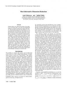
Fig. 1. The hierarchical system structure.
measurements is a good solution in some systems, especially in the wireless sensor networks where each sensor has limited computation power, there are certain cases that the raw measurements can be compressed in some more complicated ways to improve the performance. The authors in [16] presented a minimal bound of the dimension of the compressed sensor data, which could achieve the same estimation performance as using uncompressed sensor data. In other words, this bound is a “lossless” bound. The lossless compression problem was also investigated in [17]. In practice, it is not always possible and/or necessary to ensure the lossless performance. Sometimes, engineers are more concerned about the optimal compression given any system inherent constraint. This problem was studied in [19], however the results were argued to be suboptimal in [18], in which the authors further considered the fading and noisy channels in the sensor network. The algorithm provided in [18] was also suboptimal, which ensured the convergence to a stationary point. Moreover, the algorithm in [18] is computation expensive and sometimes unstable due to the matrix inversion required at each iteration. In [23], the authors addressed the measurement dimension reduction problem with knowledge of the network topology. In this paper, we consider the block-wise preprocessing and estimation problem. We aim to jointly design the preprocessors and the subsequent estimator where the preprocessors associated with each measurement block is responsible for compressing the raw data within this block to meet the inherent constraints of the system and the estimator relies solely on the compressed data for estimation. We assume that all preprocessors and the estimator are linear. It is found that there is a bound for the dimension reduction. If the permitted dimension is beyond this bound, then it is possible to design the preprocessors and the estimator to make the estimation equivalent to the linear minimum mean square error (LMMSE) estimation, which is the best that can be achieved within the linear space. In other words, there is no performance degradation incurred by the compression. However, if the required dimension reduction is below this bound, then it is impossible to achieve the LMMSE. In this case, we propose an algorithm to design the preprocessor and the subsequent estimator to minimize the mean square error (MSE) between the real “state” and the estimation. Different from most existing algorithms that can only ensure convergence to a stationary point without
performance guarantee, the proposed estimator can bound the MSE by a constant factor times the global minimum value under some additional conditions. The effectiveness of the proposed method is illustrated in different applications. It is shown in some cases that the designed preprocessors are able to compress the raw data into vectors of dimension far below the “LMMSE-achieving” bound without incurring too much performance loss. The rest of this paper is organized as follows. In Section II, the dimension reduction problem is formulated. The bound for the lossless dimension reduction is proposed in Section III and the algorithm for designing the estimator if the reduction requirement is below the bound is provided in Section IV. The performance bound of the proposed algorithm under some additional conditions is analyzed in Section V. The proposed algorithm is illustrated in three different applications in Section VI. Section VII concludes this paper. II. PROBLEM FORMULATION We consider a system where the linear measurements of states are contaminated by noise as follows (1) is the vector composed of the states of the where system, is the measurement vector, is the by measurement matrix with , and is the vector composed of the noise components. Without loss of generality, it is assumed that all the state and noise components are zero mean. In this paper, we focus on the two-level distributed state estimation problem in this system where the measurement vector is partitioned into multiple vectors ’s, and each of them is defined as a block. The measurements in one block would be preprocessed to a shorter vector before subsequent estimation. As shown in Fig. 1, each is a block and is the corresponding shorter vector by preprocessing. The subsequent state estimation will be purely based on the ’s. Assume that there is no shared measurement, i.e., each measurement is involved in only one block. Let denote the -th block, and we have , , where is the number of measurements corresponding with the -th block and denotes the transpose of . is the total number
3100
IEEE TRANSACTIONS ON SIGNAL PROCESSING, VOL. 62, NO. 12, JUNE 15, 2014
of blocks. The (1) could be re-written in the block-wise form as follows
By (3), the rows of which are all zeros correspond to the zeros in and are not necessarily kept. Therefore, the constraint on the size of is equivalent to limiting the number of nonzero rows of . According to (4) and (8), the problem of minimizing the MSE can be formulated as follows,
.. .
.. .
.. .
(2)
and are the measurement matrix and noise vector where associated with the block , respectively. We are interested in designing a distributed two-level linear estimator , , and , , where the local measurements related with block are first locally processed using , and then further processed using as follows (3) is the block preprocessed by . where Our goal is to properly design and such that the mean square error (MSE) is minimized. According to the orthogonality principle [29], we can write the MSE as follows
(4) where is the true state vector, is the output of the linear minimum mean square error (LMMSE) estimator, which is in the form of [29]
(5) where and denote the covariance matrix of and , respectively. Partitioning the corresponding matrices into sub-matrices for each block, we have , , and is the block diagonal matrix composed of , . Let us define
(6) for
and then (5) can be re-written as (7)
In (4), is a constant independent of the designed estimator. Thus, minimizing the MSE of the designed estimator is equivalent to minimizing , which can be further expanded by substituting (3) and (7) as follows (8) where
,
.
(9) where is the number of nonzero rows of and is the constraint on the size of . In other words, the designing purpose is to use to linearly combine the measurements in to reduce the size of data while preserving as much as possible useful information for the subsequent state estimation. Due to the linear measurement model , the measurements are not totally independent and thus contains some redundancy. The would serve to remove the redundancy by linearly combining them. However, the redundancy is limited, due to which there is a minimum size to represent the measurements in . It will be shown in the next section that if is beyond this size, can remove the redundancy such that the constraints are satisfied and all the useful information is preserved. If is below the minimum size, then not only the redundancy but also some useful information would be removed, incurring performance loss in the subsequent estimation. III. MINIMUM DIMENSION REQUIREMENT LOSSLESS COMPRESSION
FOR
In this section, a sufficient and necessary condition on the ’s for the system to achieve the LMMSE estimation will be shown. Before we show the condition, let us first establish an equivalent form of the problem in (9). For any given , it is always possible to use the singular value decomposition (SVD) to re-write it as [30] (10) where denote the Hermitian conjugate of . If let and , then , which means that we can always reduce to . Moreover, it is impossible to reduce below because if , then . In this case, the controversy comes that . In other words, for any given , we can always and at most reduce to , i.e., limiting is equivalent to limiting . The problem in (9) could be reformulated as
(11) Therefore, the problem of jointly designing and is equivalent to finding an optimal in the low-rank space constrained by ’s to minimize the MSE. From (11), we develop the sufficient and necessary condition on ’s for the system to achieve the LMMSE estimation. Please note that similar result with different assumptions had also been derived in Theorem 2.1 of [16].
MA et al.: DISTRIBUTED STATE ESTIMATION WITH DIMENSION REDUCTION PREPROCESSING
Theorem 1: A sufficient and necessary condition on ’s for the estimation defined in (3) constrained by (11) to achieve the global LMMSE state estimation is . Proof: First notice from (6) that . In the following, we would prove as the sufficient and necessary conditions instead. (proof of sufficiency) If , then is in the low-rank space constrained by ’s. Choose for all the blocks thus , achieving the LMMSE. (Proof of Necessity) The state estimation in (3) as a function of achieves the LMMSE if for any where is defined in (7). We will show the necessity by contradiction. Suppose there exists a block indexed such that . Let denote the dimension of the linear space , since , where and are the null spaces of and , respectively. In other words, a vector such that while . Therefore, there exists a vector such that , where is the vector with appropriate size composed of all zeros. By definition, the estimation does not achieve the LMMSE. Therefore, is a necessary condition for the estimator to achieve LMMSE. From Theorem 1, we can see that the minimum for the system to achieve LMMSE is . Taking expectation over in (2), we have , where we can see that the number of independent values in the mean of is determined by . Therefore, Theorem 1 could be interpreted that no information of the measurement is lost if is at least the number of independent components in . If we view the linear combination as projection, in case that , one tries to project the vector into a space with insufficient bases, due to which some information is lost and the LMMSE estimation cannot be achieved. IV. ESTIMATOR DESIGN FOR LOSSY COMPRESSION In the previous section, we derive a lower bound for ’s to enable the LMMSE estimator, i.e., for any dimension constraint beyond the lower bound, we can achieve the same MSE performance as the LMMSE estimator. However, in some situations where high compression ratio is needed due to, for example, high communication cost, the required dimension may be even smaller than the lower bound. In such a case, the design of the estimators will be constrained in the low-rank space, as given in (11). Obviously, the objective function is quadratic thus a convex function of , but the set is not a convex set. In this section, we proposed an algorithm to tackle this non-convex optimization problem that is guaranteed to converge. To make (11) more tractable, we first decompose the covariance matrix as follows (12) where
.
3101
We then further re-write
in the block-wise form
.. .
(13)
where . Now we can re-write the objective function in (11) as follows
(14) denotes the Frobenius norm [30] of matrix . where Since the matrices and are determined by the system parameter, they are independent of the designed estimator. Let us denote the matrix by . With , the problem in (11) can be re-written as
(15) In (15), we can see that the problem boils down to finding estimator in the low rank space to minimize the distance between and a point , where and are independent of . If is an identity matrix, the solution is trivial by discarding the most insignificant singular values of until [31]. However, for a general , there is no explicit solution. Since the problem in (15) is hard to directly solve, we seek to tackle it by formulating another optimization problem which is an approximation to the original problem (15). By introducing a new matrix , the objective function in (15) can be written as
(16) where values of
is the maximum absolute value of the eigen. Therefore, we try to solve the problem
(17) which is to minimize an upper bound of the objective function in (15). We further transform the problem in (17) using a similar idea in [32]. We replace by another parameter . This
3102
IEEE TRANSACTIONS ON SIGNAL PROCESSING, VOL. 62, NO. 12, JUNE 15, 2014
transformation gives the algorithm one more degree of flexibility in choosing to further improve the performance than fixing it to be . The problem becomes
Combining (21) and (23), the iterative steps for solving (18) can be written as follows
(24) (18) where ’s are the estimators in the low-rank constrained space and ’s are the estimators in the unconstrained space. The first term in (18) is the distance between the appropriate estimation chosen in the non-constrained space and the point that we aim to approximate in the non-constrained space. The second term is the distance between the point chosen in the non-constrained space and its projection in the low rank space. From (18), we can see that the optimal estimator is found by simultaneously minimizing two different distances through a balance factor . In such a case, we will obtain an estimator in the unconstrained space that make small, while at the same time the corresponding projection on the low rank space will not introduce too much performance degradation. In the sequel, it will be discussed in details how to solve the optimization problem and derive the performance bound. Since directly solving the optimization problem in (18) is difficult, we will solve it iteratively with two steps in each iteration: in the first step we fix and optimize , and then in the second step we optimize by fixing . For the first step, when is fixed, since the feasible set for is , the problem is a convex optimization problem, and we can derive the solution using the first order condition as follows (19) At the second step we fix in (18) and optimize it with respect to , which is equivalent to optimizing since is independent of . By Eckart-Young Theorem [31], the optimal for the problem
(20) is derived by applying low rank projection for each follows
as
where
(25) The initial point of the iteration could be easily set as . The algorithm is terminated if where is the MSE achieved by the estimator at iterations and is the pre-defined threshold. There is a tradeoff between runtime and performance in selecting . It can be seen from (24) that the proposed algorithm iteratively fixes one of and and updates the other one to minimize the cost in (18) until the termination condition is reached. Thus, it can be easily seen that the proposed algorithm always converges since the cost is always nonincreasing during the iterations and the cost is lower bounded by the LMMSE. Note that the converged solution is a stationary point and it may not be a global optimum. However, one unique characteristic of the proposed algorithm is that under some additional conditions, the MSE of the local optimal designed by this algorithm is bounded by a constant times the minimum MSE achievable by any low rank estimator satisfying the constraints in (11), which will be shown in next section. V. PERFORMANCE ANALYSIS UNDER ADDITIONAL CONDITIONS In this section, it will be shown that the convergence value of would bound the MSE by a constant times the MSE achieved by where is the estimator minimizing over the whole low-rank space . We will also show that is related with the restricted isometry constant [33] of the matrix . To show the condition, we first introduce the definition of restricted isometry constant. Definition 1: The -restricted isometry constant [33] of is defined as such that satisfying ,
(21)
(26)
where is the singular value decomposition of and is the truncated singular value matrix where only the most significant singular values are kept while all other singular values are assigned 0. The (19) can be re-written as (22)
With this definition, we are able establish a lemma that would facilitate the performance analysis of the proposed iterative algorithm. Lemma 1: Suppose the eigenvalue decomposition of is , define , then if has the -restricted isometry constant where , for any satisfying , we have
(23)
(27)
Combining (22) for all the blocks, we have
MA et al.: DISTRIBUTED STATE ESTIMATION WITH DIMENSION REDUCTION PREPROCESSING
Proof: For any we have
3103
satisfying the conditions in Definition 1, (36) Substituting
in the above equation into (35), we get
By applying the restricted isometry property (RIP), it can be further re-written as (28) To evaluate the estimator calculated by the proposed algorithm, we first define the functions (29) and (30) where to (4), as
, and . According is the MSE achieved by the estimator . Define
(31)
(37) where we have applied Lemma (1) in the first inequality since and . The last inequality is due to the fact that is the global minimizer of in the block-wise low-rank subspace thus replacing it with would increase the value. On the other hand,
is the optimal solution for the minimization In other words, problem in (15). Then we have the following theorem: Theorem 2: If has the -restricted isometry constant satisfying , then by the iterative steps in (24), (32) where
(33) satisfying the constraints in (15), we Proof: For any have . By Lemma (1), the following condition holds for any satisfying the constraints in (15)
(34) Since the is quadratic in , we could represent it by the Taylor series up to the second order as follows
(35) where
. Recall that in (24)
(38) where Lemma (1) has been used. Now subtracting (38) from (37), we get
3104
IEEE TRANSACTIONS ON SIGNAL PROCESSING, VOL. 62, NO. 12, JUNE 15, 2014
TABLE I MINIMUM ACHIEVABLE VALUES OF
FOR
SOME
Comparing it with (39) (45) where the Lemma (1) and the Cauchy-Schwarz inequality have been used in the first inequality. The second inequality is due to the RIP in (26). By the same way, the last term is bounded by
(40) Substituting (40) into (39) we can get
(41) By simplifying (41), we can get (42) where
(43) if , it is Since possible to find small enough such that making the iteration converge, and . According to (29) and (30), the MSE achieved by the estimator is (44)
where the inequality is due to that fact that is always greater than and . It is shown in the above discussions that besides an estimator design, the proposed algorithm also provides some measure based on the system parameter to evaluate the performance of the designed estimator, which is different from the existing method that can only guaranteed convergence to a stationary point [18]. Please note that the condition is only a sufficient condition for the performance analysis and it should not limit the applicability of the proposed algorithm. The convergence of the algorithm is always guaranteed independent of this condition. Moreover, sometimes it is possible to find some to make even if . From (33), since , is always greater than 1, which means that the MSE of the designed estimator is always greater than that of the optimal low-rank estimator and could provide a bound of the difference between them. This bound is related with and the -restricted isometry constant . The minimum feasible values of for some cases when are shown in Table I. For some cases, if is small, we can choose appropriate which would ensure both and to be close to 0 thus is close to 1. The MSE of the designed estimator will be close to that of the optimal estimator . However, if is relatively large, we need to choose small enough to ensure , which would make relatively large and therefore would be much greater than 1. In this case, the upper bound of performance loss provided by is loose. Nevertheless, it does not necessarily indicate the performance of the designed estimator is poor, which will be shown by numerical examples in next section. Before comparing the performance with that of the method in [18], let us first compare the computation complexity of these two methods. In Algorithm 1 of [18], it requires multiple matrix inversion at each iteration. There are two main disadvantages: first, sometimes the matrix that needs to be inverted is so close to singular that inverting it would incur a lot of inaccuracy due to which the convergence becomes an issue. Another disadvantage is that since the matrix inversion is of cubic complexity with respect to the number of measurements, this method might not be scalable. However, in the method proposed in this paper, the matrix inversion is independent of the iteration and thus does not need to be calculated each time. It makes the algorithm more robust without the risk of inverting
MA et al.: DISTRIBUTED STATE ESTIMATION WITH DIMENSION REDUCTION PREPROCESSING
3105
a matrix close to singular. Also, it reduces the complexity significantly and therefore makes it more suitable for the condition with massive measurements, especially in the case that estimators are re-designed periodically to meet the time-varying conditions. VI. APPLICATIONS There are a variety of problems in different fields using the linear measurement model in (1) where the proposed method can be applied such that the raw measurements are compressed to meet the system’s inherent constraints. If the conditions in Theorem 1 are satisfied, then the distributed LMMSE estimator can be implemented. Moreover, we are more interested in the performance of the designed low-rank estimator if those conditions can not be satisfied. In this section, three state estimation applications with inherent constraints are discussed to illustrate the effectiveness of the proposed algorithm. A. MIMO Channel Estimation To fully achieve the spatial and time diversity that MIMO systems can offer, the accurate channel state information (CSI) is required at the transmitter and/or receiver [34]. For example, the beamforming requires the CSI at the transmitter [35] while the space-time code requires the CSI at both the transmitter and the receiver [36]. While there are multiple ways to do the CSI estimation, in this example, we consider the approach using training sequence. In a MIMO system with transmitting and receiving antennas, we use the training sequence to estimate the CSI at the receiver. Namely, we consider the state estimation problem at each receiving antenna, where states are to be estimated. This estimation problem can be modeled using (1) where is the state vector of the channels from transmitting antennas to the specific receiving antenna, is composed of the received signals from time 1 up to by the receiving antenna, is the matrix composed of the training sequence from the transmitting antennas from time 1 up to and is the noise vector. Generally, the training sequence length is required to be no less then to ensure that the system is determined. In some cases, is much larger than to make the estimation less vulnerable to abnormal noise and/or interference from other devices. While the accuracy of the estimation is expected to increase with the length of the training sequence, it also brings massive measurements that the estimator need to deal with. Traditionally, the receiver would store all the measurements before using them to do the estimation. However, in some systems, the receiver side is expected to be cheap and small thus there might be not enough space for the massive measurements. We use the block-wise preprocessing to solve this problem. Instead of waiting until the end of the training sequence, the receiver would periodically preprocess the latest measurement block by a matrix to make it a shorter vector to be stored where is the index of the block. The subsequent estimation is done at the end of the training sequence when all the blocks have been received and preprocessed. Recall in (3) that the estimation is purely dependent on the preprocessed data ’s thus the raw measurement blocks can be discarded immediately after the preprocessing such that a lot of memory space can be saved.
Fig. 2. Performance of lossy preprocessing and estimation with combinations and . of
In this example, we assume that the MIMO system is equipped with 10 transmitting antennas thus the dimension of the state is 10. To ensure the performance, the training sequence of length is employed thus the total number of measurements is 40. The measurements are partitioned equally into two blocks of length 20 with the corresponding measurement matrices and where . Moreover, in this application, the is small compared with , which corresponds with the case that the system is with high measurement noise. Assume that the measurement noises are i.i.d, and without loss of generality assume that . Note that the of is bounded by in this example, which satisfies the sufficient condition in Theorem 2. To evaluate the performance of the designed estimator, we define (46) where is the state estimation obtained by the designed estimator. By (4), the MSE of the designed estimator is GAP plus a constant that is independent of the estimator design. In Fig. 2 and Fig. 3, it is shown that if the GAP is bounded by for all the cases where , which is small compared with the LMMSE that is 0.0417. It is shown that the performance of the proposed algorithm is very good such that it is able to compress the raw measurements into quite small size with little performance loss. Moreover, in Fig. 3, it is shown that the theoretical results match the simulation results obtained by Monte-Carlo simulations. The algorithm proposed in this paper is compared with Algorithm 1 in [18]. As shown in Fig. 4, the algorithm proposed in this paper has better performance than that in [18], especially in the cases where is low. Moreover, in this example, the algorithm in [18] converges within less than 10 iterations. However, the performance is not improved with more iterations. In contrast, the algorithm proposed in this paper has good enough performance with 10 iterations while at the same time the performance continues to improve, even after 1000 iterations.
3106
IEEE TRANSACTIONS ON SIGNAL PROCESSING, VOL. 62, NO. 12, JUNE 15, 2014
TABLE II THE GAP FOR THE CASES
Fig. 3. Performance of lossy preprocessing and estimation with fixed
.
Fig. 4. Comparison with Algorithm 1 in [18] with different number of iterations.
B. Power Grid In the power grid, there are generally two levels for the power to be delivered from the generation plant to household: the transmission level and the distribution level. The former delivers the power from generation plants to substations and between substations; the latter delivers the power from substations to households locally. They have quite different structures and physical properties.
,
We consider the state estimation problem in the transmission level, specifically in the IEEE 14 bus system model where there are 14 interconnected substations. Engineers are interested in the complex voltage phase differences in the substations, which is costly to directly measure. One way to get to know these states is to estimate them by power flow measurements which include the power injections at substations and the power flows in each transmission line. We assume that this system is fully measured, i.e., each substation would provide one power injection measurement while each transmission line would provide two power flow measurements, all of which are contaminated by random noise. In this system, there are 14 power injection measurements and 40 power flow measurements, while 13 phase differences are to be estimated. It can be modeled by (1) where is the measurement matrix related with the grid topology, is composed of the 54 measurements, is composed of the 13 system states and is the noise vector. In practice, the substations are usually distantly distributed. Therefore, transmitting a lot of measurements to the estimation center is expensive and sometimes even impossible. We partition the system into several groups and the measurements inside each group is preprocessed to be compatible with the transmission capability of the system. In this example, we partition the substations indexed 1,2,3,5,7,9,10 as one group while the rest as the other group. The power injection measurements are associated with the corresponding substation while the power flow measurements are associated with the originating substation. From Theorem 1, the sufficient and necessary conditions to enable LMMSE estimation is , , where and stand for the communication capability from the preprocessor of each group to the estimation center. If these conditions cannot be satisfied, the low rank estimators are designed using the proposed algorithm. By doing simulation using Matpower [37], Table II illustrates that the GAP decreases asymptotically to 0 as and increase. Moreover, it is 0 if and only if both and . Looking at the cases where both and , as shown in Table II and Fig. 5, the GAP is still close to 0 even if and are slightly below the and . It means that the estimation obtained by the low-rank estimator is quite close to the LMMSE estimation in the mean square sense. An interesting observation found in Fig. 5 is that there exists a sudden change of the GAP as and varies. Moreover, it seems like a boarder line such that if is greater than a specific value, then the GAP is insignificant compared with that when is below that value. It becomes more clear if we see the examples in Fig. 6. If , the sudden change is at ;
MA et al.: DISTRIBUTED STATE ESTIMATION WITH DIMENSION REDUCTION PREPROCESSING
3107
Fig. 5. Performance of lossy preprocessing and estimation with combinations and . of
if , the sudden change is at , and so on. The boarder line is . The reason why it is 13 is that in this system, the number of system states is 13. In other words, the estimator is using the preprocessed data with size to estimate the 13 states of the system. If , according to (3), the matrix has more rows than columns, i.e., the size of data is smaller than that of the states of the system. In this case, there is no way for any linear preprocessing to keep the linear independence of all the elements in the system state vector, i.e., to preserve enough information of all the system states. On the other hand, if , i.e., it is possible to linearly combine the measurements to preserve information of all the system states, the algorithm would always find the way to do so by designing the appropriate low-rank estimator with performance close to the LMMSE estimation. In other words, in this application, the proposed algorithm has pushed the linear preprocessing to its limit, which is to compress measurements to totally as few values as the dimension of the system, which demonstrates the effectiveness of the proposed algorithm. In Fig. 6, it is also shown that the theoretical results match the simulation results obtained by 5000 Monte-Carlo trials. In this example, the -restricted isometry constant is hard to obtain [33] and a lower bound can be provided. It is somehow surprising that . Although the condition in Theorem 2 no longer holds, the algorithm still converges. Moreover, the performance of the designed estimator is good enough. Comparing the algorithm proposed in this paper with that in [18] as shown in Fig. 7, at 10 iterations, the two methods perform really close in some cases while in other cases the proposed algorithm has better performance than that in [18]. The performance of the proposed algorithm is further improved by increasing the number of iterations from 10 to 100 while the algorithm in [18] does not have much improvement, where the proposed algorithm outperforms that in [18] in all the cases. Moreover, since it is free of matrix inversion in each iteration, the computation cost of each iteration in the proposed algorithm
Fig. 6. Performance of lossy preprocessing and estimation with fixed
.
Fig. 7. Comparison with algorithm 1 in [18] with different number of iterations.
is much lower than that in [18]. Therefore, the proposed algorithm can afford more iterations to improve the performance. C. Target Tracking Target tracking is one of the primary applications of wireless sensor network (WSN). Each sensor would observed the target and report the measurement to a fusion center for the purpose of tracking, i.e., estimating the location of the target. By combining the measurements from multiple sensors, it can be modeled using (1) where is the state containing the location information of the target, is the measurement matrix composed of the measurement matrices of all sensors, is the vector
3108
IEEE TRANSACTIONS ON SIGNAL PROCESSING, VOL. 62, NO. 12, JUNE 15, 2014
Fig. 8. Performance of lossy preprocessing and estimation with combinations and . of ,
containing the measurements from all users and is the noise vector. In reality, there are many inherent constraints in this system. For example, due to the stringent power and spectrum budget, the communication capability of the system is limited. Sometimes it is impossible for the sensor to directly report the measurements to the fusion center. One of the solutions is using the block-wise structure that the sensors are partitioned into several clusters. Each sensor first reports the measurements to a local substation within the cluster with higher communication capability that is responsible for providing information for the fusion center. However, in some applications, the communication capability of the substation is still not enough for reporting all the raw measurements. In this example, we use the proposed preprocessing method to compress the measurements reported by the sensors at the substation to meet its communication capability. Suppose that 2 targets that are randomly distributed in a particular area monitored by a sensor network composed by multiple sensors with block-wise structure, and thus the dimension of the system is 6. The sensor network is composed of sensors that partitioned into 3 clusters, each containing 10 sensors and equipped with a substation. Assume the distribution of the target and the noise are both zero-mean, with variance 5 and 0.1. We use the algorithms proposed in this paper to design the preprocessors and the estimator to satisfy the communication capability from the substation to the fusion center. In Fig. 8, it is shown that with any fixed , when both and are slightly below the lower bounds and , the GAP is close to 0. Recall in (4) that the MSE of the estimation is the sum of GAP and the LMMSE, it is still possible to estimate the target location with satisfactory MSE. For example, if , , , the GAP of the estimation is 0.0004. Since the LMMSE of this problem is 0.02, the MSE of the estimation is 0.0204 which is slightly increased. However, instead of transmitting the 30 measurements, only 9 preprocessed values are transmitted from the substations to the fusion center, saving 70% of the communication load. In Fig. 9, similar sudden changes in the GAP are observed. It is shown that if , which is the dimension of
Fig. 9. Performance of lossy preprocessing and estimation with fixed .
and
this system, the performance is satisfactory. However, if , then GAP will grow dramatically. Moreover, it also illustrates that the theoretical results match the simulation results obtained by 5000 Monte-Carlo trials. In the above, it is assumed that the target evolution model is unknown, i.e., we are doing instantaneous estimations at each time slot. However, it is worth noting that the proposed methods could be generalized to the case that the system evolution models are known. In this case, since the measurements in consecutive time slots are correlated, the proposed preprocessing method can be used to combine the measurements obtained by neighboring sensors at consecutive time slots. For example, suppose that a target is moving in a particular area that monitored by a sensor network composed by homogeneous sensors with hierarchical structure modeled by
(47) where is the state vector, is the state evolution matrix and is the system noise. is the measurement vector, is the measurement matrix composed of the measurement matrix of clusters where is the measurement matrix associated with the cluster indexed , is the noise vector. In this example, consider the preprocessing at cluster where the measurements of time instants are compressed into one single vector. By combining the states of time instants, define
.. .
(48)
MA et al.: DISTRIBUTED STATE ESTIMATION WITH DIMENSION REDUCTION PREPROCESSING
where is the states at the -th instant. The measurement model for the cluster indexed is
.. .
.. .
conditions where the estimators need to be re-designed periodically. Also, in this paper, it was assumed that the grouping of the measurements is fixed. Since different grouping may lead to quite different performance, it might also be interesting to investigate the problem of optimal grouping of the measurements. REFERENCES
.. . where stant , Define
3109
.. .
(49)
is the measurement noise in cluster at time inis the measurements in cluster at time instant .
.. .
.. .
.. .
(50)
then it can be re-written as (51) that corresponding with the model in (1) thus the proposed preprocessing method could be applied to compress the measurements. Besides using the correlation of measurements in the spatial domain, the proposed method also utilizes the correlation of the measurements in the time domain to compress them. More specifically, the measurement matrix enables us to leverage the spatial correlation between the measurements obtained by neighboring sensors. If we further have the knowledge of the temporal correlation from (47), they can be combined in (51) to compress the measurements jointly using spatial domain and time domain correlations of the measurements. VII. CONCLUSION In this paper, we addressed the problem of preprocessing the measurements to balance between the estimation accuracy and the data conciseness. It is shown that there is a bound on the compressed data size to enable lossless compression. Moreover, an algorithm to design the preprocessor and the estimator when the required size of the compressed data is below the bound is proposed. The estimator designed by the algorithm has the performance guarantee that the MSE of the estimation is at most a constant factor times the MSE of the global optimal solution under some additional conditions. Moreover, the proposed algorithm has the advantage in both robustness and computation complexity compared with existing works. Three applications are shown to demonstrate the effectiveness of the proposed method. In the future, it might be interesting to investigate distributed algorithms for designing the estimators to meet time-varying
[1] M. Lin, Y. Wu, and I. Wassell, “Wireless sensor network: Water distribution monitoring system,” in Proc. IEEE Radio Wireless Symp., Jan. 2008, pp. 775–778. [2] M. Filograno, P. Corredera Guillen, A. Rodriguez-Barrios, S. MartinLopez, M. Rodriguez-Plaza, A. Andres-Alguacil, and M. GonzalezHerraez, “Real-time monitoring of railway traffic using fiber Bragg grating sensors,” IEEE Sensors J., vol. 12, no. 1, pp. 85–92, Jan. 2012. [3] S. Massoud Amin and B. F. Wollenberg, “Toward a smart grid: Power delivery for the 21st century,” IEEE Power Energy Mag., vol. 3, no. 5, pp. 34–41, 2005. [4] A. Ribeiro and G. Giannakis, “Bandwidth-constrained distributed estimation for wireless sensor networks-part i: Gaussian case,” IEEE Trans. Signal Process., vol. 54, no. 3, pp. 1131–1143, Mar. 2006. [5] A. Ribeiro and G. Giannakis, “Bandwidth-constrained distributed estimation for wireless sensor networks-part ii: Unknown probability density function,” IEEE Trans. Signal Process., vol. 54, no. 7, pp. 2784–2796, Jul. 2006. [6] J. Yick, B. Mukherjee, and D. Ghosal, “Wireless sensor network survey,” Comput. Netw., vol. 52, no. 12, pp. 2292–2330, 2008. [7] O. Ozdemir, R. Niu, and P. Varshney, “Channel aware target localization with quantized data in wireless sensor networks,” IEEE Trans. Signal Process., vol. 57, no. 3, pp. 1190–1202, 2009. [8] K. Agrawal, A. Vempaty, H. Chen, and P. Varshney, “Target localization in wireless sensor networks with quantized data in the presence of byzantine attacks,” in 45fth Asilomar Conf. Signals, Syst., Comput. (ASILOMAR) Conf. Rec., 2011, pp. 1669–1673. [9] Z. Luo et al., “A censoring and quantization scheme for energy-based target localization in wireless sensor networks,” J. Eng. Technol., vol. 2, no. 2, p. 69, 2012. [10] Y. Zhou, C. Huang, T. Jiang, and S. Cui, “Wireless sensor networks and the internet of things: Optimal estimation with nonuniform quantization and bandwidth allocation,” IEEE Sensors J., vol. 13, no. 10, pp. 3568–3574, 2013. [11] G. Liu, B. Xu, and H. Chen, “Robust distributed estimators for wireless sensor networks with one-bit quantized data,” in Wireless Algorithms, Systems, and Applications. New York, NY, USA: Springer, 2012, pp. 309–314. [12] J. Fang and H. Li, “Power constrained distributed estimation with correlated sensor data,” IEEE Trans. Signal Process., vol. 57, no. 8, pp. 3292–3297, 2009. [13] K. Zhang, X. Li, P. Zhang, and H. Li, “Optimal linear estimation fusion—Part VI: Sensor data compression,” in Proc. 6th Int. Conf. Inf. Fusion, 2003, vol. 1, pp. 221–228. [14] Z.-Q. Luo, G. Giannakis, and S. Zhang, “Optimal linear decentralized estimation in a bandwidth constrained sensor network,” in Proc. Int. Symp. Inf. Theory (ISIT), 2005, pp. 1441–1445. [15] J. Fang and H. Li, “Joint dimension assignment and compression for distributed multisensor estimation,” IEEE Signal Process. Lett., vol. 15, pp. 174–177, 2008. [16] Z.-Q. Luo and J. Tsitsiklis, “Data fusion with minimal communication,” IEEE Trans. Inf. Theory, vol. 40, no. 5, pp. 1551–1563, 1994. [17] Z. Duan and X. Li, “Lossless linear transformation of sensor data for distributed estimation fusion,” IEEE Trans. Signal Process., vol. 59, no. 1, pp. 362–372, Jan. 2011. [18] I. Schizas, G. Giannakis, and Z.-Q. Luo, “Distributed estimation using reduced-dimensionality sensor observations,” IEEE Trans. Signal Process., vol. 55, no. 8, pp. 4284–4299, Aug. 2007. [19] Y. Zhu, E. Song, J. Zhou, and Z. You, “Optimal dimensionality reduction of sensor data in multisensor estimation fusion,” IEEE Trans. Signal Process., vol. 53, no. 5, pp. 1631–1639, May 2005. [20] K. You and L. Xie, “Kalman filtering with scheduled measurements,” IEEE Trans. Signal Process., vol. 61, no. 6, pp. 1520–1530, 2013. [21] E. Msechu and G. Giannakis, “Sensor-centric data reduction for estimation with WSNS via censoring and quantization,” IEEE Trans. Signal Process., vol. 60, no. 1, pp. 400–414, 2012. [22] K. You, L. Xie, and S. Song, “Asymptotically optimal parameter estimation with scheduled measurements,” IEEE Trans. Signal Process., vol. 61, no. 14, pp. 3521–3531, 2013.
3110
IEEE TRANSACTIONS ON SIGNAL PROCESSING, VOL. 62, NO. 12, JUNE 15, 2014
[23] N. Goela and M. Gastpar, “Reduced-dimension linear transform coding of correlated signals in networks,” IEEE Trans. Signal Process., vol. 60, no. 6, pp. 3174–3187, 2012. [24] H. Zhu, I. Schizas, and G. Giannakis, “Power-efficient dimensionality reduction for distributed channel-aware Kalman tracking using WSNS,” IEEE Trans. Signal Process., vol. 57, no. 8, pp. 3193–3207, 2009. [25] B. Aiazzi, L. Alparone, S. Baronti, and M. Selva, “Lossy compression of multispectral remote-sensing images through multiresolution data fusion techniques,” in Proc. Int. Soc. Opt. Photon. Int. Symp. Opt. Sci. Technol., 2003, pp. 95–106. [26] H. Ma, Y.-H. Yang, Y. Chen, and K. J. R. Liu, “Distributed state estimation in smart grid with communication constraints,” in Proc. Asia-Pacific Signal Inf. Process. Assoc. Annu. Summit Conf. (APSIPA ASC), 2012, pp. 1–4. [27] H. Ma, Y.-H. Yang, Q. Wang, Y. Chen, and K. Liu, “Distributed state estimation with lossy measurement compression in smart grid,” in Proc. IEEE Global Conf. Signal Inf. Process. (GlobalSIP), Dec. 2013, pp. 519–522. [28] J. Hu, J. Xu, and L. Xie, “Cooperative search and exploration in robotic networks,” Unmanned Syst., pp. 1–22, 2013. [29] B. Hajek, “An exploration of random processes for engineers,” Electr. Comput. Eng. Dept., Univ. of Illinois at Urbana-Champaign, Urbana , IL, USA, 2009. [30] R. A. Horn and C. R. Johnson, Matrix Analysis. Cambridge, U.K.: Cambridge Univ. Press, 2012. [31] C. Eckart and G. Young, “The approximation of one matrix by another of lower rank,” Psychometrika, vol. 1, no. 3, pp. 211–218, 1936. [32] R. Meka, P. Jain, and I. S. Dhillon, “Guaranteed rank minimization via singular value projection,” 2009 [Online]. Available: http://arxiv.org/ abs/0909.5457, abs/0909.5457. [33] B. Recht, M. Fazel, and P. A. Parrilo, “Guaranteed minimum-rank solutions of linear matrix equations via nuclear norm minimization,” SIAM Rev., vol. 52, no. 3, pp. 471–501, 2010. [34] K. J. R. Liu, A. K. Sadek, W. Su, and A. Kwasinski, Cooperative Communications and Networking. Cambridge, U.K.: Cambridge Univ. Press, 2009. [35] A. Sadek, W. Su, and K. J. R. Liu, “Transmit beamforming for spacefrequency coded MIMO-OFDM systems with spatial correlation feedback,” IEEE Trans. Commun., vol. 56, no. 10, pp. 1647–1655, 2008. [36] W. Su, Z. Safar, M. Olfat, and K. J. R. Liu, “Obtaining full-diversity space-frequency codes from space-time codes via mapping,” IEEE Trans. Signal Process., vol. 51, no. 11, pp. 2905–2916, 2003. [37] R. Zimmerman, C. Murillo-Sánchez, and R. Thomas, “Matpower: Steady-state operations, planning, and analysis tools for power systems research and education,” IEEE Trans. Power Syst., vol. 26, no. 1, pp. 12–19, Feb. 2011.
Yu-Han Yang (S’06) received his B.S. in electrical engineering in 2004, M.S. degrees in computer science and communication engineering in 2007, from National Taiwan University, Taipei, Taiwan, and Ph.D. degree in electrical and computer engineering in 2013 from University of Maryland, College Park, USA. His research interests include wireless communication and signal processing. He received Class A Scholarship from the ECE department, National Taiwan University in Fall 2005 and Spring 2006. He is a recipient of Study Abroad Scholarship from Taiwan (R.O.C.) government in 2009–2010. He received the University of Maryland Innovation Award in 2013.
Hang Ma (S’10) received his B.S. degree in information engineering from Northwestern Polytechnical University, Xian, China, in 2010. He is currently pursuing the Ph.D. degree at University of Maryland, College Park, USA. His research interests include wireless communication and signal processing. He received the honor of Outstanding Graduate of Northwestern Polytechnical University in 2010.
Qi Wang received his B.S. degree in electrical and information engineering from Xidian University, Xi’an, China, in 2011. He is currently pursuing the M.S. degree at University of Maryland, College Park, USA. His research interests include Neural Networks and Deep Learning. He received first class honor of graduate students of Xidian University in 2011.
Yan Chen (S’06–M’11) received the Bachelor’s degree from University of Science and Technology of China in 2004, the M. Phil degree from Hong Kong University of Science and Technology (HKUST) in 2007, and the Ph.D. degree from University of Maryland College Park in 2011. His current research interests are in data science, network science, game theory, social learning and networking, as well as signal processing and wireless communications. Dr. Chen is the recipient of multiple honors and awards including best paper award from IEEE GLOBECOM in 2013, Future Faculty Fellowship and Distinguished Dissertation Fellowship Honorable Mention from Department of Electrical and Computer Engineering in 2010 and 2011, respectively, Finalist of Deans Doctoral Research Award from A. James Clark School of Engineering at the University of Maryland in 2011, and Chinese Government Award for outstanding students abroad in 2011.
K. J. Ray Liu (F’03) was named a Distinguished Scholar-Teacher of University of Maryland, College Park, in 2007, where he is Christine Kim Eminent Professor of Information Technology. He leads the Maryland Signals and Information Group conducting research encompassing broad areas of signal processing and communications with recent focus on cooperative and cognitive communications, social learning and network science, information forensics and security, and green information and communications technology. Dr. Liu was a Distinguished Lecturer, recipient of IEEE Signal Processing Society 2009 Technical Achievement Award and various best paper awards. He also received various teaching and research recognitions from University of Maryland including university-level Invention of the Year Award; and Poole and Kent Senior Faculty Teaching Award, Outstanding Faculty Research Award, and Outstanding Faculty Service Award, all from A. James Clark School of Engineering. An ISI Highly Cited Author, Dr. Liu is a Fellow of IEEE and AAAS. Dr. Liu is Past President of IEEE Signal Processing Society where he has served as President, Vice President C Publications and Board of Governor. He was the Editor-in-Chief of IEEE SIGNAL PROCESSING MAGAZINE and the founding Editor-in-Chief of EURASIP Journal on Advances in Signal Processing.