1
Distributed synchronization of noisy non-identical double integrators Ruggero Carli, Alessandro Chiuso, Senior Member, IEEE , Luca Schenato Member, IEEE , Sandro Zampieri Abstract— In this paper we present a novel synchronization protocol to synchronize a network of controlled discrete-time double integrators which are non-identical, with unknown model parameters and subject to additive measurement and process noise. This framework is motivated by the typical problem of synchronizing a network of clocks whose speeds are non-identical and are subject to variations. This synchronization protocol is formally studied in its synchronous implementation. In particular, we provide a completely distributed strategy that guarantees convergence for any undirected connected communication graph, and we also propose an optimal convex design strategy when the underlaying communication graph is known. Moreover, this protocol can be readily used to study the effect of noise and external disturbances on the steady-state performance. Finally, some simulations including also asynchronous implementation of the proposed algorithm are presented.
I. I NTRODUCTION The extraordinary success of Internet and of wireless technologies has created the opportunity to interconnect a huge number of devices which can exchange information and cooperate to accomplish new tasks and to control the environment more effectively. One important problem to be solved in many applications involving a network of distributed devices, such as in wireless sensors networks (WSNs), is to maintain them temporally synchronized. The main challenges in time synchronization for networked clocks are due to random communication delay among devices, to the unknown, non-identical and often time-varying periods of each clock oscillator, and to the unknown topology of the network. Moreover, there might not be a reference clock in the network. Many synchronization protocols have already been proposed and experimentally tested, in particular for WSNs. A common approach is to create a hierarchical structure such a directed tree where each clock synchronizes itself with respect to its parent. The challenge with this approach is to dynamically elect a root and reconstruct the tree whenever nodes fail or new nodes appear, as proposed by Ganeriwal et al. [4] and Maroti et al. [6] for example. Another hierarchical approach is to divide the network into distinct clusters, each with an elected cluster-head. All nodes within the same cluster synchronize themselves with the corresponding cluster-head, and each cluster-head synchronizes itself with a another cluster-head, as described by Elson et al. [2]. These hierarchical approaches however require substantial overhead to build the dynamic trees or clusters and might not scale well for very large networks. More recently, totally distributed synchronization protocols have been proposed where each node in the network runs exactly the same algorithm irrespective of This work has been supported by the project FeedNetBack funded by the European Community, by WISE-WAI project funded by CaRiPaRo Foundation, by the national project Sviluppo di nuovi metodi e algoritmi per l’identificazione, la stima bayesiana e il controllo adattativo e distribuito funded by MIUR and Progetto di Ateneo CPDA090135/09 funded by the University of Padova. Ruggero Carli is with the Center for Control, Dynamical Systems and Computation, University of California at Santa Barbara, Santa Barbara, CA 93106, USA.
[email protected] Alessandro Chiuso is with the Department of Management and Engineering, Universit`a di Padova, Stradella S. Nicola, 3 - 36100 Vicenza, Italy, ph. +39049-8277709, fax. +39-049-8277699, e-mail:
[email protected] Luca Schenato and Sandro Zampieri are with the Department of Information Engineering, Universit`a di Padova, Via Gradenigo, 6/b, 35100 Padova, Italy. e-mail:{schenato,zampi}@dei.unipd.it
the size or topology of the network, such as those proposed by Solis et al. [11] and Schenato et al. [10]. In this work we present a novel distributed synchronization protocol which is based on a second order linear consensus algorithm. The term consensus refers to a general class of distributed algorithms that allow multiple agents to converge to the same quantity of interest using only local communication. This class of algorithms has been successfully applied to many applications such as flocking, coordinated formation control and distributed estimation (e.g. see [8]). As in [11] and [10] our proposed protocol is fully distributed, however it has the advantage to use a simple linear output feedback strategy which allows performance analysis also in the presence of measurement and process noise. In fact, the protocol in [11], which is based on the cascade of two distributed least-square algorithms, and the protocol in [10], which is based on the cascade of two first order consensus algorithms, are both nonlinear and do not lead to simple characterization of performance in the presence of noise. Time synchronization of clocks with different speeds provides an interesting class of systems. In fact, each local clock can be modeled as the output of a double integrator whose rate in not perfectly known. Moreover this rate is slightly different from one clock to another, therefore even if all clocks are perfectly synchronized at one time, they will slowly diverge from each other if no compensation or resynchronization is applied. Synchronization can be modeled as the tracking of the average of external signals with linear growth, namely local clocks without compensation. Work in the context of signal tracking with consensus algorithms have been proposed, among others, by Spanos et al. [12], Freeman et al. [3], and Zhu et. al [16]. However these works are in continuous time with no noise and do not provide optimization strategies for the protocol parameters. The presence of noise has been explicitly taken into account by Xiao et al. [15], but only for first order consensus dynamics. Differently, synchronization of networked higher order systems is a more recent topic of research. Most of the available results are for synchronization of either non-identical systems which are strictly stable [5], or identical linear systems [9],[13]. More challenging is the problem of stabilizing unstable systems. Specific attention has also been given to the synchronization of double integrators which are unstable systems with a ramp mode [7]. However these strategies strongly rely on the assumption that all systems are identical and no optimization is performed. In this paper we first propose a distributed clock synchronization protocol based on the consensus algorithm for non identical double integrators whose rates of growth are not known nor measurable. This technique is only analyzed in the unrealistic synchronous implementation. Motivated by this application, the main contributions of the present paper reside in the extension of the optimization techniques proposed by Xiao et al. [15] for first order consensus protocols to consensus protocols for double integrators. More specifically, we propose centralized optimization algorithms for optimally designing the protocol parameters both in terms of rate of convergence and in terms of steady state error in case the protocol is perturbed by an additive noise. Interestingly, this last optimization problem shows that the optimal design strategy requires the optimization of a convex function of all the consensus matrix eigenvalues, thus being quite different from the standard procedure which suggests to minimize the second largest eigenvalue of the consensus matrix. Finally, we include some simulations where we compare the performance of the synchronous implementation with a randomized asynchronous implementation. These simulations seem to suggest that the solution we propose is effective also in its more realistic asynchronous version, even though we do not have at the moment any theoretical evidence of this fact.
2
II. M ODELING AND MOTIVATIONS Assume we have N units and that each unit i has a clock which is an oscillator able to periodically increment a register by one unit, commonly known as tick. We assume that the periods ∆i of these oscillators are unknown, but are “perturbed” values of a “nominal” and known period ∆. Therefore, the value of the i-th register is 0i τi (t) = ⌊ t−t ⌋, where the “floor” ⌊a⌋ indicates the largest integer ∆i smaller than or equal to a, and t0i denotes the time when the clock has been started. The unit has to use these ticks in order to estimate time. Since only the nominal clock period ∆ is known, the natural time estimate is yi (t) = ∆τi (t) + yi (t0i ) (II.1) where yi (t0i ) is the initial offset which is an estimate of t0i . Since the ∆i ’s are all different, then each clock will drift away from the others even under the ideal situation in which they are all initially synchronized, i.e., yi (0) = yj (0) for all i, j. Therefore some sort of information exchange and clock control must be enforced to obtain and maintain synchronization among all nodes. If we assume that the nodes periodically exchange their clock readings yi (t) at times t = hT , where h = 0, 1, . . . and T ∈ R is the synchronization period, then they can use them to adjust their clock estimate yi (t) so that eventually all nodes will be synchronized, i.e., yi (t) ≃ yj (t) for all i, j. A natural approach to achieve synchronization is to control the nominal clock period ∆ and the clock offset yi (0) based on the information received from the neighboring nodes. As a preliminary step, let us observe that the evolution of yi (hT ) in (II.1) can be described through the following iterative algorithm – – » » yi (0) 1 ∆δi (h) xi (h), xi (0) = xi ((h + 1)T ) = 1 0 1 ˆ ˜ yi (hT ) = 1 0 xi (hT )
where xi (hT ) ∈ R2 and where δi (h) := τi ((h + 1)T ) − τi (hT ). If x′i and x′′i denote the two components of xi , then x′i gives the time estimate, while ∆x′′i gives the oscillator period estimate. For sake of conciseness, with no loss of generality we will assume in the sequel that T = 1. Each node can use any information it receives from the neighboring nodes at time hT = h to insert a control in the previous iterative algorithm – » 1 ∆δi (h) xi (h)+ui (h) (II.2) xi (h+1) = 0 1 ˆ ˜ yi (h) = 1 0 xi (h). (II.3)
Notice that δi (h) = τi ((h + 1)T ) − τi (hT ) = 1/∆i + ǫ(h) where −1 < ǫ(h) < 1 and so ǫ(h) can be neglected if 1/∆i >> 1 which will be assumed in the sequel. Notice moreover that the previous system corresponds to the output of a second order integrator with unknown parameter, since ∆i is not known. Moreover, the dynamics of each clock is different since in general ∆i 6= ∆j . We propose here a linear control law of the following structure ui (h) = −F
N X
kij (h)yj (h)
(II.4)
j=1
where kij (h) is the i − j entry of the matrix K(h) ∈ RN×N , F ∈ R2×1 , and we assume that communication and computational delays are negligible. Notice that at time hT the protocol requires the transmission of the output yj (h) from the node j to the node i if and only if kij (h) 6= 0. The problem is to determine the matrix F and the matrices K(h) such that all the yi (h)’s converge to the same ramp shaped function.
Assume now that K(h) = K for all h and that K1 = 0, where 1 is the N -dimensional column vector with all entries equal to 1. Without loss of generality we can assume F = [f1 f2 ]T = [1 α]T since f1 can be absorbed into K so that α := f2 /f1 . Introduce finally the 2N dimensional vector x(h) having x′ (h) := [x′1 (h), . . . , x′N (h)]⊤ as the first N entries and having x′′ (h) := [x′′1 (h), . . . , x′′N (h)]⊤ as the second N entries. Then the previous equations can be collected in the following – » ′ x (0) x(h + 1) = AD x(h), x(0) = 1 – » (II.5) I−K D AD := −αK I where I ∈ RN×N is the identity matrix, D = diag{ ∆∆1 , . . . , ∆∆N }, and x′ (0) ∈ RN . Our objective is to find K and α such that the synchronization error defined as: e(h) = [Ω 0]x(h)
(II.6)
with Ω = I − N1 11∗ , converges to zero while the components of x′ (h) follow asymptotically a ramp function, i.e. limh→∞ [x′ (h) − (ah + b)1] = 0 for some a ∈ R+ , b ∈ R. Therefore the problem we tackle in this paper can be formulated as follows. Determine K and α such that: a) system (II.5) has one eigenvalue in 1 with algebraic multiplicity 2 and geometric multiplicity 1. This ensures that the state trajectories contains the modes of the form ah + b; b) the two modes associated with the eigenvalue 1 are unobservable with respect to output e defined in (II.6); c) all the other eigenvalues are inside the open unit disk; d) possibly some cost function (depending on K and α) is minimized. ˆ ˜⊤ For conditions a) and b) observe that, if we let v := 1⊤ 0 ˆ ˜ ⊤ and w := 0 1⊤ D−1 then we have that (AD − I)w = v
(AD − I)v = 0
showing in this way that v and w are respectively an eigenvector and a generalized eigenvector of AD in (II.5) associated with the eigenvalue 1. Notice moreover that [Ω 0]w = [Ω 0]v = 0, which shows that they are both unobservable. Remark 2.1: The strategy proposed by Scardovi and Sepulchre in [9] for obtaining consensus for higher order systems is not applicable for time synchronization. Indeed for their method we have that in the non ideal case in which D 6= I, the eigenvalue 1 becomes observable and so we do not obtain consensus. We need now to find methods able to give K and α satisfying conditions c) and d) of the previous list. Observe preliminarily that often the ∆i ’s are slightly different and can be seen to be a small perturbation of the nominal value ∆. Therefore the dynamics of Eqn. (II.5) can be seen as the perturbation of the system where D = I. Concerning condition c), observe that, since the eigenvalues are continuous function of the matrix elements, if we find a solution satisfying condition c) letting D = I, this solution will continue to satisfy that condition even in case that D is a small enough perturbation of I. Similarly for condition d), if the cost function to be minimized is continuous in D, then the optimal solution found assuming D = I will have approximately the same cost of the optimal solution obtained starting from the true D. For these reasons, in the stability analysis and in the optimization problems which will follow, we will assume that D = I. We will use the symbol AI for the matrix AD in (II.5) when D = I.
3
III. S TABILITY ANALYSIS The aim of this section is to study under which conditions on K and α the proposed synchronization algorithm yields e(h) converging to zero; this is equivalent to require that AI := AD |D=I in (II.5) has two eigenvalues in 1, as as seen before, while all the other eigenvalues belong to the open unit disc. For simplicity, in the sequel we will assume that K is symmetric. Let U be an orthogonal matrix formed with the eigenvectors of K, i.e., such that U ∗ KU = Λ where Λ = diag {λ1 , λ2 , . . . , λN } is the diagonal matrix containing the eigenvalues λi of K. Since K1 = 0, without loss of generality we will assume that λ1 = 0. Proposition 3.1: Consider the system (II.5) in the case where D = I. Then the remaining 2N − 2 eigenvalues of this system are inside the open unit disk if and only if 0 4α max |1 − λ/2 1 ± 1 − 4α/λ | As mentioned above, we have to minimize the largest of the r(λ, α)’s as λ varies in σ(K) \ 0, where σ(K) denotes the spectrum of K. Hence we define R(K, α) :=
max
λ∈σ(K)\0
r(λ, α)
(IV.2)
The optimal values of α and K are the solution of the optimization problem {Kopt , αopt } ∈ arg min R(K, α) (IV.3) K∈K, α∈(0,1)
where we recall that K is the set of rank N − 1, symmetric, positive semidefinite matrices compatible with the given graph and such that K1 = 0. Being of rank N − 1 is equivalent to the fact that λ2 (K) > 0. Notice that only matrices in K can yield stabilizing controllers and that, as observed in Proposition 3.2, such a set is nonempty if the supporting graph is connected. Define now KN as the subset of K formed S only by the matrices such that λ2 (K) = 1. Notice that K = β>0 βKN . This implies that the previous optimization is equivalent to the following one ¯ opt , αopt , βopt } ∈ {K
arg min
¯ K∈K N , α∈(0,1), β>0
¯ α) R(β K,
(IV.4)
since αopt here is the same as in Eqn. (IV.3) and since Kopt = ¯ opt . The optimization problem (IV.4) will now be considered. βopt K Tedious but straightforward computations yield to the following results which are summarized as a lemma. Lemma 4.1: The following facts hold true: a) The function r(λ, α) is decreasing in λ for λ < 4α and it is increasing in λ for λ > 4α. b) The value of R(K, α) depends on K only through its smallest λ2 and largest λN nonzero eigenvalues. More precisely we have R(K, α)
=
max{r(λ2 , α), r(λN , α)} =: F (α, λ2 , λN )
4
Root Locus
3.5
1
Imaginary Axis
3 0.5
2.5 2
0 1.5
β
1
−0.5
opt
0.5 −1 −1
−0.5
0
Real Axis
0.5
1
0 0
0.5
1
1.5
2
β
2.5
3
3.5
4
4.5
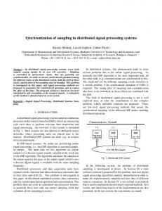
Fig. 1. Root locus of (z − 1)2 + λ(z − 1 + α) = 0 for α = 1/3 as a function of λ ∈ [λ2 , λN ].
¯ opt ), α) with α = 0.3 and Fig. 2. The graphs of r(β, α) and of r(βλN (K ¯ opt ) = 1.5 λN (K
c) For fixed α and λ2 , the function F (α, λ2 , λN ) is nondecreasing in λN . ¯ ∈ KN , α ∈ (0, 1) and β > 0 the condition Since, for any K ¯ α) = F (α, β, βλN (K)) ¯ holds, then a direct consequence of R(β K, ¯ opt in (IV.4) is given by item (c) in the previous lemma is that K
y(h) = v(h) so that, inserting the control (II.4) in equations (II.2) and (II.3), a term of the form – » K v(h) αK
¯ opt ∈ arg min λN (K). ¯ K
(IV.5)
¯ K∈K N
Note that the set KN is not convex but (IV.5) can be equivalently reformulated as the following convex optimization problem1 ¯ opt ∈ K
arg min
¯ ¯ K∈K, λ2 (K)≥1
¯ λN (K).
(IV.6)
¯ opt ) = 1. If this was not true, i.e. λ2 (K ¯ opt ) > 1, Note that λ2 (K ′ ¯ opt /λ2 (K ¯ opt ) would give a lower cost ¯ opt := K then the matrix K ′ ′ ¯ opt )/λ2 (K ¯ opt ) < λN (K ¯ opt ) and λ2 (K ¯ opt ¯ opt ) = 1, ) = λ N (K λ N (K ¯ opt . against the optimality assumption of K Thus the optimization problem (IV.4) is decoupled into the cascade of (IV.6) above followed by ¯ opt )). {αopt , βopt } ∈ arg min F (α, β, βλN (K
(IV.7)
α∈(0,1),β>0
Problem (IV.6) is a convex optimization problem since (i) the ¯ is a convex and symmetric spectral function (see objective λN (K) ¯ ∈ K, λ2 (K) ¯ ≥ 1} is convex set. In e.g. [1]) and (ii) the set {K particular (IV.6) can be formulated as a semi-definite program (SDP) for which standard and efficient software is available. ¯ opt has been found, we need to find αopt and βopt solving Once K (IV.7). To this aim, notice that ¯ opt )) = max{r(β, α), r(βλN (K ¯ opt ), α)} F (α, β, βλN (K and so, for fixed α and as a function of β, it is the maximum between ¯ opt ), α) (see Figure 2). r(β, α) and its stretched version r(βλN (K For the properties of the function r(λ, α) mentioned in Lemma 4.1, this function is minimized for the unique β such that r(β, α) = ¯ opt ), α) and so this equation gives βopt (α) which can be r(βλN (K found for instance using a bisection method. Finally, the optimal value of α can be found via a linear search for α ranging in the interval (0, 1). V. N OISY MODEL In this section we will consider a noisy version of Eqn. (II.5). First of all, we allow for noisy measurements y(h) of the form x′ (h) − 1 This
optimization it can performed using the techniques proposed in [14].
has to be added on the right hand side of (II.5). In addition we allow for a model noise to act on the second component of the state2 , thus obtaining – – » » 0 K n(h), (V.1) v(h) + x(h + 1) = AI x(h) + I αK where v(h) and n(h) are assumed ˆto be uncorrelated white noises ˜ with zero mean and covariances E n(t)n⊤ (τ ) = qIδ(t − τ ) and E [v(t)v ∗ (τ )] = rIδ(t − τ ). We will also assume that, for all h ≥ 0, both n(h) and v(h) are uncorrelated from the initial condition x(0), which is assumed to be random. For clearness of exposition, a motivation of the model noise n(h) in the clock synchronization problem will be given in Appendix A. Clearly the presence of the noise prevents in general that e(h) → 0. Therefore, in order to evaluate how much the performance of the algorithm degrades, we introduce the cost functional ˆ ˜ 1 J(K, α) := lim sup E ke(h)k2 (V.2) N h→∞
where the expectation is taken over the initial condition and the realizations of the noises. The cost J can be expressed as a function of α and of the eigenvalues λi as formalized in the following lemma. Lemma 5.1: Let J be defined as in (V.2) and let λ1 , . . . , λN be the eigenvalues of K. Under the conditions (III.1) and (III.2) in Proposition 3.1 the cost J(K, α) satisfies: N „ 1 X (α2 − 3α + 2)λh + 2α J(K, α) = r+ N h=2 (1 − α)(4 − (2 − α)λh ) « (α − 1)λh + 2 q (V.3) + α(1 − α)(4 − (2 − α)λh )λ2h
Proof: As we have seen in Section II the system (II.5) has an unobservable component with two eigenvalues in 1. Under the assumptions of Proposition 3.1, all other eigenvalues are stable. Thus, restricting to the (stable) observable component of the state, the proof follows from a rather standard application of Ljapunov equations to compute the steady state covariance in linear state space models and is omitted in the interest of space. 2 It should be observed that since we consider a double integrator, it would make little sense to add a model noise term also in the first component of the state.
5
The goal now is to design K and to choose α in order to minimize J(K, α), i.e. to solve arg min
J(K, α),
(V.4)
α∈(0,1), K ∈ K
where K is the set of symmetric positive semidefinite matrices introduced in the previous section. Observe that, from the proof of Lemma 5.1 it follows that, if the conditions (III.1) and (III.2) are not satisfied, then J(K, α) := +∞. Now, given α, let K(α) = {K ∈ K : λN < 4/(2 − α)} .
(V.5)
In other words K(α) is the set of positive semidefinite matrices compatible with the graph structure, satisfying K1 = 0 and ensuring that, given α such that 0 < α < 1, the cost functional J(K, α) is finite. The minimization problem (V.4) can be treated in the following way. We start by observing that ` ´ min J(K, α) = min J K opt (α), α , α∈(0,1), K ∈ K
α∈(0,1)
opt
where K (α) ∈ arg minK ∈ K(α) J(K, α). Assume now α fixed. We have the following proposition. Proposition 5.2: Fix α ∈ (0, 1) and let K(α) be defined as in (V.5). Then the function J(K, α) defined on K(α) is a convex function. Proof: Consider the function f : B → R defined as N „ X (α2 − 3α + 2)xh + 2α f (x1 , . . . , xN ) = r+ (1 − α)(4 − (2 − α)xh ) h=2 « (α − 1)xh + 2 + q (V.6) α(1 − α)(4 − (2 − α)xh )x2h ˘ ¯ where B = x ∈ RN : 0 < xi < 4/(2 − α) . We show that f (x1 , . . . , xN ) is convex. To this aim consider the h-th term in the summation in the right-hand side of (V.6). Observe that (α2 −3α+2)xh +2α is a convex hyperbola for xh ∈ ]0, 4/(2 − α)[. (1−α)(4−(2−α)xh ) Moreover » (α − 1)xh + 2 1 1 α = + 2+ α(1 − α)x2h (4 − (2 − α)xh ) α(1 − α) 8xh 2xh – (2 − α)α + 8(4 − (2 − α)xh ) where each term of the summation in the right-hand side of the above expression is convex for xh ∈ ]0, 4/(2 − α)[. Hence the function f is convex in B. Finally observe that the function f is symmetric, i.e., it is invariant to any permutation of the vector entries xh . Hence, it follows from the theory of convex spectral functions [1] that also J is a convex function. From the above proposition, and from the fact that the set K(α) is a convex set, it follows that the minimization problem K opt (α) ∈ arg min J(K, α)
(V.7)
K ∈ K(α)
is a convex optimization problem. In particular the solution of (V.7) can be obtained by suitable numerical algorithms. Once (V.7) has been solved, one is left with ` ´ arg min J K opt (α), α α ∈ (0,1)
which reduces to a linear search over α and is easily solved. VI. N UMERICAL EXAMPLES
In this section we provide two examples illustrating the approach proposed in this paper. Specifically, in Example 6.1 we simulate the algorithm described in Section II in a time-varying setup, while in
Example 6.2 we deal with the minimization problems formulated in Section IV and in Section V. Example 6.1: In Section II the convergence properties of the synchronization algorithm illustrated in Section II have been characterized, under the assumption that K is time-invariant. The goal of this example is to show the effectiveness of this synchronization algorithm also in a time-varying setup. To do so, we propose a comparison between the synchronous implementation given in (II.5) and a randomized asynchronous implementation, based on a broadcast communication protocol, that we describe next. Let G be a generic undirected graph. To the graph G we can associate the doubly stochastic (Metropolis) matrix PM etr , built as illustrated in Eqn. (III.4), and the corresponding matrix KM etr := I − PM etr . Assume now that at each time instant a node of G is randomly chosen with a probability 1/N . Without loss of generality let i be the node chosen at time h and let us denote by Ni the set of its neighbors in G. At time h, node i broadcasts the value x′i (h) to all the nodes in Ni . The neighboring nodes j ∈ Ni update their state using the input uj (h) := [1 α]T kji (x′j (h) − x′i (h)), where kji denotes the element of the j-th row and i-th column of KM etr . For all nodes ℓ which are not neighbors of node i, i.e. ℓ ∈ / Ni we set uℓ (h) = 0. In more compact form the matrix K(h) can be written as “ ” X K(h) = kji ej eTj − ej eTi . (VI.1) j∈Ni
Observe that E[K(h)] = N −1 KM etr . In Figure 3, we show the behavior of the synchronization error both for the synchronous implementation given in (II.5) and for the asynchronous implementation described above for a connected random geometric graph generated by choosing N = 15 points uniformly distributed in the unit square and by connecting with an edge each pair of points at distance less than 0.4. Notice that in the asynchronous implementation only one node transmits its information at each time instant. For this reason, in order to make a fair comparison, when analyzing the asynchronous implementation we sample the value of the synchronization error every N iterations of the algorithm. To be more precise, in Figure 3, we plot in dashed line the quantity Js (h) := log √1N kes (h)k, where es denotes the synchronization error for the synchronous implementation, in solid line the quantity Ja (h) := log √1N kea (N h)k, where ea denotes the synchronization error for the asynchronous implementation. The synchronous algorithm in (II.5) has been implemented with K = KM etr and α = αM etr , where αM etr = minα∈(0,1) R(KM etr , α). In the asynchronous algorithm we built K(h) as in (VI.1) and we fixed α = αM etr /N . The factor 1/N in α used in the asynchronous implementation is related to the fact that the N asynchronous steps should be compared with one synchronous, as discussed above. As far as the initial condition is concerned, the speeds of the clocks (i.e., the elements of the matrix D) and the initial local time (i.e., the values x′i (0), i ∈ {1, . . . , N }) have been chosen randomly in the intervals [0.9, 1.1] and [0, 100], respectively. Moreover the plot reported is the result of the average over 1000 Monte Carlo runs, randomized with respect to both the graph and the initial conditions. The results obtained show the effectiveness of the randomized asynchronous implementation whose performance turns out to be comparable with the performance of the synchronous one. Example 6.2: In this example we analyze numerically the optimization problems formulated in (IV.4) and in (V.4). To this aim, we introduce the following nomenclature. Given a connected undirected
6
200 10
J
a
150
s
JMetr
J
0
100
−5
10
50 0 0
−10
5
10
10
0
50
100
150
200
h
250
300
350
400
450
15
20
25
400
Fig. 3. Behavior of the synchronization error both for the synchronous implementation and asynchronous implementation. Metr
300
200
τ
graph G, let
JOpt
ROpt = min R(K, α), α∈(0,1) K∈K
JOpt = min J(K, α),
100
α∈(0,1) K∈K
where R and J have been defined in (IV.2) and in (V.3), respectively. Now, we associate with the graph G the matrix PM etr , built as illustrated in (III.4). Let KM etr := I − PM etr and define RM etr := R(KM etr , α = 1/2)
0 0
20
τ
Opt
40
60
Fig. 4. Plot of the points (JOpt , JM etr ) (upper). Plot of the points (τOpt , τM etr ) (lower).
JM etr := J(KM etr , α = 1/2). which correspond to the performance of the totally distributed design strategy proposed in Proposition 3.2. We run 30 experiments. At each experiment, we generated a connected random geometric graph, as in the previous example. For all the experiments we set the value of the parameters q and r, i.e., the variances of ni (t) and vi (t), equal to 1. We plotted the points (JOpt , JM etr ) and the points (τOpt , τM etr ) log 0.05 log 0.05 3 where τOpt = log in the upper figure and , τM etr = log ROpt RM etr in the lower figure of Figure 4, respectively. In order to facilitate the comparison we also plot the bisector straight lines. As expected, in both cases, all the points lie above these lines. Moreover, observe that, in most cases, the improvement gained by choosing the optimal matrix K is considerable for both cost functionals. VII. C ONCLUSIONS We have presented a second-order consensus algorithm for a family of non-identical double integrators which borrows tools from standard control theory and consensus algorithms. The main motivation comes from clock synchronization in a network of agents. The optimal controller for fastest rate of convergence in this class can be formulated as a convex optimization problem. Linearity also allows to perform a rather simple analysis of the effect of the noise on the asymptotic performance. While the analysis has been performed for a synchronous algorithm, numerical simulations show that an asynchronous implementation of the same algorithm has a comparable performance to the synchronous one. Indeed an important research direction is the theoretical analysis of asynchronous algorithms and their testing in real networks of clocks.
are time varying functions, it is reasonable to write D in Eqn. (II.5) as D(h) = I + S(h) i . It is reawhere S(h) = diag {Si (h)}i=1,..,N , Si (h) := ∆−∆ ∆i sonable to model the terms Si (h) as a random walk, i.e. Si (h) = Si (h − 1) + ni (h). The noises ni (h) enters in the model in a multiplicative manner since Si (h) multiplies the second state component x′′i (h). However x′′i is always approximately equal to one4 and hence it is reasonable to assume Si (h)x′′i (h) ≃ Si (h). Under this approximation, and redefining the second component of the state as x′′i (h) + Si (h), we obtain the term – » 0 n(h) I
on the right hand side of (V.1), where ni (h) is the i-th component of n(h). R EFERENCES
(respec-
[1] J.-M. Borwein and A.-S. Lewis. Convex Analysis and Nonlinear Optimazation. CMS Books in Mathematics. Canadian Mathematical Society, 2000. [2] J. Elson, L. Girod, and D. Estrin. Fine-grained network time synchronization using reference broadcasts. In Proceedings of the 5th symposium on Operating systems design and implementation (OSDI’02), pages 147– 163, 2002. [3] R. Freeman, P. Yang, and K.M. Lynch. Stability and convergence properties of dynamic average consensus estimators. In 45th IEEE Conference on Decision and Control (CDC’06), pages 398–403, San Diego, December 2006. [4] S. Ganeriwal, R. Kumar, and M. Srivastava. Timingsync protocol for sensor networks. In Proceedings of the first international conference on Embedded networked sensor systems (SenSys’03), 2003. [5] C.-Y. Kao, U. T. Jonsson, and H. Fujioka. Characterization of robust stability of a class of interconnected systems. To appear in Automatica.
) gives the asymptotic number of steps for the tively the synchronization error decreasing of a factor ǫ when K = KOpt (respectively when K = KM etr ).
4 In the practical implementation x′′ is kept bounded in an interval of the i form [1 − ǫ, 1 + ǫ] to avoid dangerous drifts.
A PPENDIX A In the context of clock synchronization the process noise n(h) in (V.1) can be justified as follows. Assuming that the clock’s periods ∆i 3 Note
that, given an positive real number ǫ, the quantity ǫ quantity log log RM etr
log ǫ log ROpt
7
` [6] Mikl`os Mar`oti, Branislav Kusy, Gyula Simon, and Akos Ldeczi. The flooding time synchronization protocol. In Proceedings of the 2nd international conference on Embedded networked sensor systems (SenSys’04), pages 39–49, 2004. [7] W. Ren. On consensus algorithms for double-integrator dynamics. IEEE Transactions on Automatic Control, 53(6):1503–1509, 2008. [8] R. Olfati Saber, J.A. Fax, and R.M. Murray. Consensus and cooperation in multi-agent networked systems. Proceedings of IEEE, 95(1):215–233, January 2007. [9] L. Scardovi and R. Sepulchre. Synchronization in networks of identical linear systems. Automatica, 45(11):2557–2562, 2009. [10] L. Schenato and F. Fiorentin. Average timesync: A consensus-based protocol for time synchronization in wireless sensor networks. In Proceedings of 1st IFAC Workshop on Estimation and Control of Networked Systems (NecSys09), September 2009. [11] R. Solis, V. Borkar, and P. R. Kumar. A new distributed time synchronization protocol for multihop wireless networks. In 45th IEEE Conference on Decision and Control (CDC’06), pages 2734–2739, San Diego, December 2006. [12] D. Spanos, R. Olfati-Saber, and R.M. Murray. Dynamic consensus on mobile networks. In Proceedings of the 16th IFAC World Congress, July 2005. [13] P. Wieland, J.-S. Kim, H. Scheu, and F. Allgower. On consensus in multi-agent systems with linear high-order agents. In Proc. 17th IFAC World Congress, pages 1541–1546, 2008. [14] L. Xiao and S. Boyd. Fast linear iterations for distributed averaging. Systems and Control Letters, 53:65–78, 2004. [15] L. Xiao, S. Boyd, and S.-J. Kim. Distributed average consensus with least-mean-square deviation. Journal of Parallel and Distributed Computing, 67(1):33–46, 2007. [16] M. Zhu and S. Martinez. Discrete-time dynamic average consensus. Automatica, 46(2):322–329, 2010.