Geosci. Model Dev., 9, 383–392, 2016 www.geosci-model-dev.net/9/383/2016/ doi:10.5194/gmd-9-383-2016 © Author(s) 2016. CC Attribution 3.0 License.
Distributed visualization of gridded geophysical data: the Carbon Data Explorer, version 0.2.3 K. A. Endsley1,2 and M. G. Billmire1 1 Michigan 2 School
Tech Research Institute (MTRI), Michigan Technological University, Ann Arbor, MI, USA of Natural Resources and Environment (SNRE), University of Michigan, Ann Arbor, MI, USA
Correspondence to: K. A. Endsley (
[email protected]) Received: 24 June 2015 – Published in Geosci. Model Dev. Discuss.: 23 July 2015 Revised: 14 January 2016 – Accepted: 15 January 2016 – Published: 29 January 2016
Abstract. Due to the proliferation of geophysical models, particularly climate models, the increasing resolution of their spatiotemporal estimates of Earth system processes, and the desire to easily share results with collaborators, there is a genuine need for tools to manage, aggregate, visualize, and share data sets. We present a new, web-based software tool – the Carbon Data Explorer – that provides these capabilities for gridded geophysical data sets. While originally developed for visualizing carbon flux, this tool can accommodate any time-varying, spatially explicit scientific data set, particularly NASA Earth system science level III products. In addition, the tool’s open-source licensing and web presence facilitate distributed scientific visualization, comparison with other data sets and uncertainty estimates, and data publishing and distribution.
1
Introduction
Today’s scientific enterprise must consider the challenges and opportunities associated with the growing scale of scientific observations, the need for scalable analyses, and the benefits and obligations of sharing scientific outputs. In climate models, in particular, a wealth of observations can be generated or collected but rich, collaborative insight requires additional frameworks and software tools. Hence, there is a renewed emphasis in the Earth system sciences on tools and best practices for the documentation and sharing of analyses, metadata generation (e.g., Earth System Documentation, ESDOC), and scientific provenance (e.g., The Kepler Project; Altintas et al., 2004).
In this paper, we describe a new, web-based framework for managing, analyzing, and collaboratively visualizing Earth system science data sets: the Carbon Data Explorer (http: //spatial.mtri.org/flux-client/), version 0.2.3. Although the tool’s intended use is for carbon science data sets (e.g., regional carbon flux, global carbon concentration), the Carbon Data Explorer is compatible with any time-varying, spatially explicit Earth system data set or model output (e.g., land surface temperature, evapotranspiration, aerosol optical thickness). We present the tool as a prototype system that addresses the challenges of increasing scientific data volumes, the need for online analysis, and the desire to share results with collaborators. Commensurate with the growth of computing power, geophysical models are producing data with increasingly fine spatial and/or temporal resolution (Nativi et al., 2015). Considering the spatial and temporal dimensions within a data set simultaneously can be demanding both on computational resources and on a scientist’s ability to manage and visualize results. As a conceptual aid, a spatiotemporal data set consisting of only one parameter of interest can be visualized as a three-dimensional data cube (Fig. 1), a representation commonly used in scientific computing (Alder and Hostetler, 2015). The three-dimensional data cube metaphor should not be taken to mean that visualizations of the data cube are necessarily 3-D. Rather, the minimum three dimensions of the data cube include the two axes of a Cartesian coordinate system and an additional axis for time. The data cube representation has also gained traction in recent scientific visualization tools; UV-CDAT (Santos et al., 2013) and Panoply (Schmunk, 2015) are two examples.
Published by Copernicus Publications on behalf of the European Geosciences Union.
384
K. A. Endsley and M. G. Billmire: The Carbon Data Explorer, version 0.2.3
Figure 1. A three-dimensional data cube in which spatial data of two dimensions (e.g., latitude and longitude) are combined with a third dimension of time. In this view, a horizontal slice perpendicular to the time (t) axis corresponds to a geographic map while a line parallel to the time (t) axis represents a time series.
The Carbon Data Explorer also adopts the data cube as a functional interface for high-volume spatiotemporal data. A map view of a single point in time can be visualized as slicing the data cube perpendicular to the time (T ) axis and parallel to the geographic (X–Y ) plane. Conversely, a time series display at one point in space (one pair of geographic coordinates) can be visualized as a narrow threading along the time axis and perpendicular to the X–Y plane. For multivariate data we must begin to construct and think in terms of higherdimensional data hypercubes. The Carbon Data Explorer is agnostic as to the type of data contained in data cubes and can simultaneously accommodate any number of variables. While data cubes work well for storing scientific data offline, web browsers and web applications are designed to work largely with plain text documents (interpreted variously as HTML, XML, JavaScript, or other documents). Non-text formats can be downloaded directly from an online directory or through File Transfer Protocol (FTP). Indeed, many scientists, unable to procure or unaware of a more sophisticated solution, provide large collections of outputs directly through FTP – essentially a networked folder available to the public. Indexing, searching, or manipulating data must then be done offline. As an alternative, open application programming interface (API) standards such as the Open Geospatial Consortium (OGC) Web Map Service (WMS) allow two computers – a web browser and a remote web server – to communicate about data through an agreed-upon protocol (Blower et al., 2013). WMS, as an example, allows web applications to find tiled map images such as those that form the background of modern, interactive web maps like Google Maps. The Opensource Project for a Network Data Access Protocol (OPeNDAP) is another protocol that describes how hierarchical data files (HDFs) and Network Common Data Form (NetCDF) Geosci. Model Dev., 9, 383–392, 2016
files, among other file types, are stored and accessed (Cornillon et al., 2003). Thus, dissemination of scientific data on the web typically requires a metadata-driven API or resource descriptor framework (RDF); these are implemented as a kind of textbased communication protocol that describes (to a computer) where binary data can be found and how they can be accessed. This enables web applications to ultimately retrieve and display data in formats that are not native to the web. However, these APIs incur considerable performance costs when online analysis of data sets is required or when representations are generated dynamically from incoming, realtime data streams (e.g., Sun et al., 2012; Alder and Hostetler, 2015). The Carbon Data Explorer solves this problem by introducing a new API for text-based representations of data cubes, thereby enabling easy integration with and high performance in browser-based web applications while also providing capabilities for dynamic querying, aggregation, differencing, and anomaly calculations. This text-based representation is not only compatible with web browsers, it allows for the data to be manipulated directly in the website, providing asynchronous rapid filtering and aggregation. Only the OGC Web Coverage Service (WCS), a protocol also based in a data cube metaphor, allows for this level of interaction and online analysis of data (OGC, 2016). However, in our experience, stand-alone WCS implementations are usually undocumented or the documentation is relegated to the WCS standard. The adoption of web APIs for sharing data is further evidence of the scientific community’s desire to share results with a wider audience. In addition, the ubiquity of social media is bringing online conversations about science, albeit informal, and there are even emerging social networks dedicated to scientific discourse and exchange (e.g., ResearchGate, Academia.edu). This unprecedented interconnectivity is also motivated by best practices in collaborative science. The next phase of the Climate Model Intercomparison Project, CMIP6, will for the first time allow “anyone at any time [to] download model data for analysis” (Meehl et al., 2014). As part of CMIP5, the Earth System Grid Federation (ESGF) provides a unified gateway to scientific data sets hosted anywhere in the world. Thus, the ability to share and compare model results should motivate the further development of web-compatible scientific analyses. In response to this need, the Carbon Data Explorer allows data providers to share scientific data sets, analyses, and visualizations directly on the web. A data provider might be a modeler, the principal investigator of an interdisciplinary research team, or a technician or information technology (IT) professional embedded in a research team. NASA estimates that these scientists and model developers spend more than 60 % of their time preparing model inputs and model intercomparisons (as cited by Rood and Edwards, 2014). The Carbon Data Explorer was designed specifically to enable cliwww.geosci-model-dev.net/9/383/2016/
K. A. Endsley and M. G. Billmire: The Carbon Data Explorer, version 0.2.3 mate modeling outputs to be brought online, visualized, and compared. In its capacity as a data management and data access web server, the Carbon Data Explorer is similar to the THREDDS Data Server (TDS); its analytical capabilities make it similar to Ferret-THREDDS. The Carbon Data Explorer expands on both by providing an integrated front-end for visualization and analysis. While the THREDDS Client Catalog requires data to be registered with XML descriptors, the Carbon Data Explorer Python API has a user-friendly command-line interface that allows for faster, repeatable, one-time registration of data without the need to open a text editor and write XML. In data interchange, it also substitutes bulky XML for lightweight and more human-readable JavaScript Object Notation (JSON). In addition, it eschews the vulnerability-prone Java environment and Tomcat web server for a light-weight, nonblocking web server in Node.js that can be hidden behind a proxy server such as Apache. This design choice trades off the protocol interoperability of TDS, which was not identified as a requirement by our user community, for the ease of development and deployment of web services with newer, JavaScript-based technologies on the server. The scientific data sets supported by the Carbon Data Explorer include any gridded or non-gridded time-varying, spatially explicit data that can be decomposed into one variable at a time. The canonical example of a supported data set is any NASA level III scientific data product, defined as “variables mapped on uniform space–time grid scales” (NASA, 2010). These geophysical variables are usually derived from satellites (e.g., OCO-2) or models, reanalysis data sets and global or regional Earth system models. Many scientific data sets, particularly level III products, are already stored as binary (flat) files or in complex, hierarchical data structures (e.g., NetCDF or HDF) that were designed to accommodate data cubes (Blower et al., 2013). The Carbon Data Explorer shares similar aims with technologies such as NASA’s World Wind virtual globe, Giovanni, and Mirador. Compared with World Wind, the Carbon Data Explorer provides access to analytical capabilities that would be awkward or impossible to reproduce in a virtual globe. Also, unlike World Wind, it requires neither a stand-alone installation nor a dependency library such as Java and runs in any web browser. While Mirador allows users to download spatially explicit scientific data sets from NASA missions, it has no analytical or visualization capabilities. The Carbon Data Explorer most closely resembles Giovanni in that both are web-based, map-centered viewers. While Giovanni provides more sophisticated analytical capabilities, the Carbon Data Explorer is designed to deliver results faster and allows for greater customization of the visualization and the querying of measurement values within the web client. In sum, the Carbon Data Explorer is intended for more rapid examination and comparison of climate model outputs by the modelers themselves.
www.geosci-model-dev.net/9/383/2016/
385
In common with the Earth System Grid Federation (Williams et al., 2009), the Carbon Data Explorer aims to provide a common environment for the access to and analysis and visualization of Earth system science data sets. The ability to quickly load spatially explicit scientific data in a web browser allows for the online querying and comparison of measurement values at specific locations across data sets and the rapid, online filtering and aggregation of measurement data. These features are not currently available in Giovanni and alternative data management frameworks and web servers, such as TDS – particularly those that provide only rasterized data representations, such as WMS – are not capable of delivering this level of analysis or speed of interactivity. We expect that these and other features of the Carbon Data Explorer make it a useful contribution to the emerging frameworks for data analysis and intercomparison. The remainder of the paper discusses these and other technical details and describes the full suite of features available. 2 2.1
Technical description Data sources
In the development and evaluation of the tool, we relied heavily on some reference data sets exemplary of those we intend to support. These included a 1-degree-by-1-degree carbon flux estimate at 3 h time steps from the NASA Carnegie Ames Stanford Approach (CASA) model run with Global Fire Emissions Databaset (GFED) input data and 1degree-by-1-degree carbon concentration (XCO2 ) data at 6day time steps modeled by the Carnegie Institution for Science’s Department of Global Ecology at Stanford University (http://dge.stanford.edu/labs/michalaklab/CO2DAAD/). The CASA–GFED model outputs included monthly uncertainty estimates; the XCO2 data were gridded by kriging from biascorrected XCO2 retrievals. 2.2
Implementation
The Carbon Data Explorer has three main components: a Python API for data management, a web server API, and a client-side JavaScript web application (Fig. 2). From a data provider’s perspective, data enter a pipeline from creation to visualization on the web beginning with the Python API, which transforms and stores the data in a database. The data are then automatically available on the web (or a local area network) through the server API and can be viewed and shared through the web application. This suite of software could be run on a single computer or separately on multiple computers, each running any UNIX-like operating system (Mac OS X or a GNU/Linux system). The suite is designed to be installed on the data provider’s (modeler’s) network, with the server API optionally facing the public web. The Python programming language (version 2.7) was chosen as the framework for data management, manipulation, Geosci. Model Dev., 9, 383–392, 2016
386
K. A. Endsley and M. G. Billmire: The Carbon Data Explorer, version 0.2.3
Figure 2. A unified modeling language (UML) deployment diagram for the Carbon Data Explorer (CDE), illustrating the configuration and connections between the components as currently deployed.
and storage due to its high-level language design, wide adoption in the scientific community, and available open-source libraries. In particular, as many scientific products are stored as HDF or early Matlab files, Python provides fast and robust support for reading scientific data products through the NumPy (Van Der Walt et al., 2011) and SciPy (Jones et al., 2015) libraries. We also expect that Python provides an environment that many data providers are already familiar with or can learn easily should they need to extend the data management API to support new or customized data sets. The web server and web client are both implemented in JavaScript. This was a strategic but also practical decision. JavaScript is fast and expressive. It is also the de facto language of the web; the only language that is natively supported by every modern web browser (Crockford, 2008). While JavaScript is not widely used for scientific computing, no experience with the language is needed to use the Carbon Data Explorer. We selected Node.js (http://nodejs.org/) as the framework for running a JavaScript server because it provides event-driven request handling, which, like multithreading, can significantly speed up server response time for most web applications (Tilkov and Vinoski, 2010). Performance testing of the Carbon Data Explorer was conducted using Apache JMeter. For each of the requests listed in Table 1, 10 identical, repeated queries were sent to the server over 30 s. Tests were done sequentially and were performed three times with several hours to several days between the runs to ensure general results.
Geosci. Model Dev., 9, 383–392, 2016
2.3
Data management and storage
Open data APIs for science capitalize on storing and sharing text-based metadata associated with scientific data that are stored in a binary or hierarchical format. We took this a step further and designed a data model that is text-only; that is, the format of the data both on-disk and when transmitted over the web is plain text. Specifically, the data are stored and transmitted as JSON documents. These JSON documents are stored in a MongoDB database instance, which handles indexing and retrieval of plain-text representations. MongoDB is one of several document-oriented databases capable of storing semi-structured data as key-value pairs. As the goal was to get the data on the web, we chose MongoDB for its transparent, text-based storage. Alternatives such as Apache Hadoop and Cassandra, while offering performance advantages, do not provide a clear pathway for rendering binary files as text. These alternatives may faithfully and rapidly operate on chunks of the data but would require that input binary files be split and transformed into some kind of operational format for handling in a map-reduce framework. As no obvious intermediate format was known at the time of development, we opted for a format that most closely resembled the output representation – the native, text-based representation required for the web browser – as the intermediate format to be stored and operated on in the database. This design choice trades off performance for flexibility and the operational demands of bringing data in binary files onto the web. Array databases such as PostGIS, a spatial extension to the relational database management system (RDBMS) Postwww.geosci-model-dev.net/9/383/2016/
K. A. Endsley and M. G. Billmire: The Carbon Data Explorer, version 0.2.3
387
Table 1. Results of load testing in Apache JMeter; network speeds are in seconds to request completion. The off-network tests were performed over a wireless internet connection; on-network tests were performed with a wired, direct network connection to the server.
Request
Data extent and resolution
Grid structurea Grid structureb Gridded X–Y datac Gridded X–Y datad Temporal aggregation, 40 X–Y gridse Temporal aggregation, 40 X–Y gridsf Time series at X–Y pointg Time series at X–Y pointh Time series for region, 684 cellsi Time series for region, 684 cellsj
North America, 1-by-1 degrees World, 1-by-1 degrees North America, 1-by-1 degrees World, 1-by-1 degrees North America, 1-by-1 degrees World, 1-by-1 degrees North America, 1-by-1 degrees World, 1-by-1 degrees North America, 1-by-1 degrees World, 1-by-1 degrees
Mean return speed, s (n = 30) Off-network On-network 0.17 0.44 0.14 0.34 0.49 2.90 0.10 0.75 0.12 0.79
0.03 0.08 0.02 0.12 0.36 2.31 0.06 0.62 0.08 0.72
Request URIs: a /api/scenarios/casa_gfed_2004/grid.json; b /api/scenarios/r2_xco2_kriged/grid.json; c /api/scenarios/casa_gfed_2004/xy.json?time=2004-05-01T03:00; d /api/scenarios/r2_xco2_kriged/xy.json?time=2009-06-15T00:00; e /api/scenarios/casa_gfed_2004/xy.json?start=2004-05-01T03:00&end=2004-05-06T03:00 &aggregate=positive; f /api/scenarios/r2_xco2_kriged/xy.json?start=2009-06-01T00:00&end=2010-02-01T00:00 &aggregate=positive; g /api/scenarios/casa_gfed_2004/t.json?coords=POINT(-50.5+69.5)&start=2004-05-01T03:00 &end=2004-05-02T03:00; h /api/scenarios/r2_xco2_kriged/t.json?coords=POINT(-50.5+69.5)&start=2009-06-15T00:00 &end=2009-08-05T00:00; i /api/scenarios/casa_gfed_2004/t.json?start=2004-05-01T03:00&end=2004-05-02T03:00 &interval=hourly&geom=POLYGON((-97+46,-101+37,-93+35,-89+42,-97+46)); j /api/scenarios/r2_xco2_kriged/t.json?start=2009-06-15T00:00&end=2009-08-05T00:00 &geom=POLYGON((-97+46,-101+37,-93+35,-89+42,-97+46))
greSQL, are another alternative to MongoDB that we considered. The use of an array database would have satisfied the need for an intermediate format – in this case, array stores – but for the purposes of enabling in-client manipulation of the data (e.g., querying measurement values, changing the stretch) this approach would have required the transformation of requested data to another format, likely text. Based on the authors’ experience with PostGIS, there were also no clear performance advantages to array databases. Thus, a document-oriented database like MongoDB allows the latency associated with preparing scientific data for the web to be pushed offline, during initial registration and insertion of the data to the database. In addition, MongoDB features an aggregation pipeline, which allows us to make sophisticated queries such as net carbon flux over the last 16 days. The web server API, which facilitates connections to the MongoDB instance, contains libraries that enable further sophistication with queries, applying fast arithmetic operations for queries such as the difference between carbon concentration (in ppm) today and this day last year. Users can shuttle scientific data into and out of the MongoDB instance by directly interacting with the Carbon Data Explorer Python API classes or by using a set of accompanying command line tools designed to ease workflow. Command line tools are available for querying database contents as well as for loading, renaming, and removing data sets from the database. When loading a data set, its metadata must be
www.geosci-model-dev.net/9/383/2016/
specified either via command line argument or via an accompanying JSON file. Examples of required metadata parameters include column identifiers, grid resolution, units, starting timestamp, and time step length. These metadata parameters inform the correct methods for transforming and querying the data for use within the web server API. The metadata also encode population summary statistics, which are calculated by the Python API during insertion to MongoDB, to aid in visualization (e.g., calculating a stretch). The transformation of data from binary or hierarchical flat files to a database representation is facilitated by two Python classes, models and mediators, which are loosely based on the transformation interface described by Bulka (2001). The Model class is a data model that describes what a scientific data set looks like; i.e., whether it is a time series of gridded maps or a covariance matrix, for instance. The Mediator class describes how a given Model should be read from and the data it contains translated to a database representation. Some basic Mediator and Model classes are provided in the Python API. It is expected that data providers with a particular output format can easily create new Model and Mediator subclasses to seamlessly read and write data to and from the MongoDB database and the files in which their data are currently stored. Transforming heterogeneous data to a uniform structure is a typically onerous task. In developing the interface for storing data in MongoDB, we aimed for a flexible system predicated on sensible defaults. The Model class of the Python
Geosci. Model Dev., 9, 383–392, 2016
388
K. A. Endsley and M. G. Billmire: The Carbon Data Explorer, version 0.2.3
API defines how measurement values can be read from any file interface available in Python. This flexibility was also driven by the historical development of related software systems. For instance, we discovered that Matlab has changed the format of its saved binary output files over the years from a proprietary data structure to one that is compatible with HDF5 (MathWorks, 2015). We selected Python and its essential SciPy library as together they provide support for Matlab, HDF4, and HDF5 formats. Thus, our experience is a reminder of the importance of backwards compatibility, which is likely well-recognized in the scientific programming community. Scientific data in the Carbon Data Explorer are conceived of as belonging to a particular run of a scenario, i.e., a specific geophysical modeling objective. Data cube(s) are stored as one or more scenarios. During data insertion to MongoDB, the X–Y slices at all time points are stored as separate documents. Each scenario has one timeline associated with it and gridded data belonging to that scenario are uniquely keyed by their date and time. Non-gridded data are assigned arbitrary unique identifiers, making it possible to have two pieces of non-gridded data that represent the same instance in time (or span of time) associated with the same scenario. At the present time, the Carbon Data Explorer supports only structured grids; that is, the gridded data in a scenario must share the same uniform, rectangular grid. Measurement values are stored and transmitted independent of the spatial reference information, eliminating redundancies and allowing for rapid retrieval and display on the web. The X–Y values associated with gridded data – the spatial coordinates of each data point – are stored separately and transmitted only once to the web application. In contrast, non-gridded data are stored with their X–Y values and transmitted as GeoJSON, a spatially explicit form of JSON, as their spatial structure may vary. 2.4
Provision of scientific data on the web
The Carbon Data Explorer web server API is designed to work out-of-the-box so that data can be served and visualized with the web application on any web browser connected to the same local area network. That is, any user on the same network as the computer running the server can access the Carbon Data Explorer through its internet protocol (IP) address in their web browser. Data providers might choose to host the Carbon Data Explorer locally so as to keep their data private and collaborate internally. Deploying the server and web application on the public web is also easy, though it may require some familiarity with networking technology. The web server makes data available as resources that are each associated with a uniform resource identifier (URI). The model used for organizing these resources in a single namespace (i.e., under a single host or domain name) is the Representational State Transfer (REST) model (Fielding and Taylor, 2000), in which different representations of data are proGeosci. Model Dev., 9, 383–392, 2016
visioned with semantics. For example, a list of all available scenarios can be obtained at, e.g., /scenarios.json as a JSON document. Alternately, the metadata for a single scenario, e.g., the casa_gfed_2004 scenario, can be obtained at /scenarios/casa_gfed_2004.json. As another example, a map of carbon flux on 18 January 2004 at 03:00 UTC from the casa_gfed_2004 scenario can be obtained at /scenarios/casa_gfed_2004/xy.json?time=2004-0118T03:00 where xy refers to the X–Y values from our data cube (i.e., a geographic map). This distinguishes map data from a time series, which could be requested in JSON format from the t.json resource, e.g., t.json?start=2003-12-22T03:00&end=2005-0101T00:00&aggregate=mean&interval=daily. While the t.json endpoint could be conceived of as delivering multiple 2-D maps (X–Y slices), it actually delivers a 1-D time series. This is because fully-2-D time series were not required for any of the features identified by the user community and would be expensive to generate. The aggregate and interval keywords, which designate the statistic and bin size of the aggregation, respectively, are required parameters that describe how multiple 2-D maps are collapsed into a 1-D time series. These limited examples showcase only a small part of the functionality of the web server’s API (Table 2). These relatively human-readable URIs allow for experienced users to download data directly if preferred. They are also used behind-the-scenes in the web application to programmatically request data as indicated by a user through its graphical user interface (GUI). The RESTful design of the web server’s API underscores an important point about having scientific data directly available in the user’s web browser. We believe scale changes, changes in the palette, and similar changes are in the purview of the client application; as they are merely changes in the application’s state, they should be performed asynchronously in the client application without requiring interaction with the remote server. Keeping data on the server requires that new representations are generated even for relatively minor changes in application state. One example is the seamless rescaling of the visualization, e.g., changing the stretch on-the-fly. We have seen performance issues in comparable approaches to this problem, e.g., with WMS, which must request the data again from the server whenever scaling changes are desired. While similar tools such as Giovanni have also enabled seamless changes to visualization parameters, they do not allow for map-based querying of measurement values or simultaneous comparison of measurement values across data sets, as the Carbon Data Explorer does.
www.geosci-model-dev.net/9/383/2016/
K. A. Endsley and M. G. Billmire: The Carbon Data Explorer, version 0.2.3
389
Table 2. Entry points for the Carbon Data Explorer web server API. Web server API entry point
Description
/scenarios.json /[scenario]/grid.json /[scenario]/xy.json /[scenario]/t.json
Requests metadata for all or selected data sets Requests a GeoJSON representation of the scenario’s X–Y grid Requests data values corresponding to the scenario’s spatial grid Requests time series data
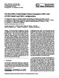
Figure 3. Screenshot of the Carbon Data Explorer web browser application in the Single Map View mode.
3
Features
In the Carbon Data Explorer client application, a rich user interface (Fig. 3) provides users many options for visualizing, exploring, comparing, and ultimately sharing geophysical data that have been previously imported with the Python API and made available to the client through the web server API. In Table 3 and in the subsequent text, we highlight some of the chief features available to users. A demonstration video (doi:10.5281/zenodo.18941) of the web browser application can also be seen through a link on the project website (http://spatial.mtri.org/flux/). 3.1
Spatial visualization and analysis
The default view in the Carbon Data Explorer client application is the Single Map View, which displays a geographic view (an X–Y slice) of the data at a particular time. The Map Settings define the map projection used (currently a choice between Equirectangular or Mercator) and what kind of base map should be drawn (e.g., continents with or without political boundaries). When gridded data are drawn on the map, the Symbology options allow a user to specify a color palette from a selection of colorblind-safe, perceptually linear color scales designed by Brewer (2014). Both sequential and diwww.geosci-model-dev.net/9/383/2016/
verging color scales are available for linear data that are either constantly increasing or are diverging from a threshold or mean value, respectively. The number of bins in the color scale can also be specified. While the default stretch of the data to the color scale is a standard deviation about the mean, both the measure of central tendency and the number of standard deviations can be changed. As an alternative to this stretch, the scale can be stretched to the domain of the data or any arbitrary endpoints as entered by the user. A binary map can also be shown, where a single color is used to code for grid cells or data points that fall within a userspecified range. The Single Map View allows the user to explore the data as in a geographic information system (GIS). Users can zoom into the map display, pan the map around, and query the value of a data point by hovering over it with the cursor. Nongridded data can be plotted on top of gridded data and automatically share the same color scale. An optional border drawn around the non-gridded data points can help to distinguish them from the gridded data. This feature allows, for example, the direct comparison of gridded carbon concentration with bias-corrected retrievals from atmospheric sounding. Data can be quickly aggregated in time or space from within the web application. The temporal aggregation is han-
Geosci. Model Dev., 9, 383–392, 2016
390
K. A. Endsley and M. G. Billmire: The Carbon Data Explorer, version 0.2.3
Table 3. List of features (present when marked with an X) in the two visualization modes of the Carbon Data Explorer web browser application. Category
Feature
Single map view
Coordinated view
Mapping
Gridded data map display Non-gridded data map display Basemap selection Map projection selection Map zoom and pan View multiple map frames simultaneously View global/ continental/ regional data
X X X X X
X
X
X X X X X
Symbology
Color palette selection Scaling, stretching, and thresholding
X X
X X
Analysis
Animation Map pixel querying Temporal queries and aggregation Spatial queries and aggregation Time series line plot Display difference of two maps Side-by-side comparison
X X X X X X
Data export (as image or GIS file) Browser remembers settings Shareable URI/URL generation
X X X
Sharing
dled by the MongoDB aggregation pipeline, which facilitates very fast aggregation of multiple X–Y slices (maps spanning time). Spatial aggregation of one or more pixels (an aggregate value spanning a spatially filtered subset) is achieved using a combination of the JavaScript Topology Suite (JSTS) Topology Suite JavaScript library and MongoDB’s geospatial query operators. Both temporal aggregation and differencing are handled by the MongoDB aggregation pipeline. The calculation and display of anomalies is done client-side in JavaScript. All other visualization tweaks and statistical stretching are done on-the-fly in JavaScript. Spatial filters can be drawn directly on the map interface or imported as polygons defined using GeoJSON or wellknown text (WKT), a human-readable representation of geometry. Currently, only a single polygon can be used at a time. Map data can also be differenced – one X–Y slice can be subtracted from another (from a different scenario and same time or vice-versa). This may help in identifying deviation from a seasonal trend or other anomalies as well as help in identifying differences between different models or different model runs of the same time step. 3.2
Time series analysis
While in the Single Map View, the map can be animated in time, updating its display (at time T ) with the next X– Y slice from our data cube. This update is seamless when the web server API is hosted on the same local network or when viewed over a high-speed internet connection, making Geosci. Model Dev., 9, 383–392, 2016
X
X
a refresh rate of one second practical for quickly reviewing model results at a rate of a few hours, days, or months every second (depending on the temporal resolution of the data). A slower animation speed can be selected for a more moderate pace. This high data throughput is made possible by the text-based data format discussed earlier. Aggregates and differenced data can also be animated in time. A line plot at the bottom of the map shows the global time series for the currently viewed scenario by default; it is the aggregate mean value across the X–Y domain at each point in time. This provides an overview of the overall trend in the data across the spatial domain. When a spatial filter is applied, an aggregate time series for only that region can be generated. The non-aggregate time series for a specific pixel can also be obtained by clicking on that grid point in the map. Retrieval of a time series data for the line plot is slower than other data requests but it still returns results in seconds. 3.3
Multiple-time and multiple-model comparison
The coordinated view allows for comparison of multiple adjacent map views; it is essentially a grid of multiple Single Map View elements. These maps synchronize their extent whenever the user pans or zooms so that the same portion of the globe is displayed in each one. The user’s cursor will now display not just the value of a data point in one map but the value at that those spatial coordinates in every map facilitating pixel-to-pixel comparison across the maps. Up to nine (9) maps can be viewed at once, which allows for nine www.geosci-model-dev.net/9/383/2016/
K. A. Endsley and M. G. Billmire: The Carbon Data Explorer, version 0.2.3 different time points or nine different models to be viewed simultaneously. 3.4
Other features
A user’s Map Settings, Symbology, and other global settings are stored in the web browser so that, upon closing the browser and returning to the web application later, the same color scale, map projection, and other settings are automatically applied. This allows users to customize their view of a data set and their workspace within the tool. All of these settings can also be encoded as a URI (or URL). This allows specific views of a data set to be bookmarked or shared with others over the web. With this feature, a user can apply a specific color scale, stretch (or threshold to highlight a particular anomaly), or an aggregate or differenced model result and then share a link that ensures that their team member will see the data exactly the same way. This is similar to the virtual variables of Ferret-THREDDS but provides not only access to an analysis but also access to a client for visualizing and interacting with that analysis. For offline storage and sharing of results, model visualizations and data slices can be exported as image files, CSVs (for non-gridded data), or as geospatial data (for gridded data) in the form of ESRI ASCII Grid files or GeoTIFFs; the latter two formats enable model results to be downloaded and opened in a desktop GIS like ArcGIS or QGIS.
4
Concluding remarks
The Carbon Data Explorer is presented as a prototype for a comprehensive data management, analysis, visualization, and sharing framework for Earth system science data sets, particularly gridded spatiotemporal data sets (e.g., NASA level III data products). As with any design, there are inherent trade-offs. In prioritizing client-side queries and analysis for regional and global-scale climate data (e.g., 1-degreeby-1-degree), this design will not scale to higher-resolution data sets, particularly those derived from moderate resolution satellite sensors (e.g., MODIS products at 1 km ground sample distance). Future iterations of the Carbon Data Explorer and similar software tools can meet the challenge of increasing spatial resolution by combining support for clientside vector features with conventional raster imagery services (e.g., Web Coverage Service, OPeNDAP, THREDDS). The authors hope that the Carbon Data Explorer serves such future integrations as a model for best practices in client-side interaction, analysis, and visualization. In order to accommodate high-resolution data sets in the future, later versions of the Carbon Data Explorer will need a radically redesigned back-end, incorporating the scalability of alternatives such as Apache Hadoop or Cassandra, and the development of a text-based HTTP response middleware. A future tool that makes these scalable back-ends operational for rapid, clientwww.geosci-model-dev.net/9/383/2016/
391
side queries and analysis in a user-friendly web application, informed by visualization best practices (as with the Carbon Data Explorer), which accommodates high-resolution geophysical data, would be a significant advance. The Carbon Data Explorer contains all the tools necessary for online scientific data analysis in one package, including a non-blocking web server, an extensible, light-weight API, and a user-friendly web application. The text-based JSON format for storage and data interchange is not only fundamentally compatible with web browsers, but also allows for scientific data to be manipulated in the web browser, providing asynchronous, rapid filtering, and aggregation. In response to the new protocols of CMIP6, the Carbon Data Explorer provides a framework for the distributed analysis of climate model outputs. Analyses can effectively be bookmarked with URIs serving as permanent links to a particular visualization and analysis of a data cube at a given point in time. The framework’s open-source licensing and web integration enable the visualization and sharing of scientific data through either a secure network or public portal. Also, as a prototype, it is hoped that the software’s seamless, interactive visualization and comparison features will inspire the expansion of existing data management and data access frameworks such as TDS and Ferret-THREDDS to support more rich, JavaScript-based visualization libraries. It is hoped they will also facilitate the future improvement of the Carbon Data Explorer and the inspiration of similar and better tools for Earth system science. Code availability The source code is available from GitHub (https://github. com/MichiganTechResearchInstitute/CarbonDataExplorer) under the MIT license. A built version of the web browser application (flux-client) is available upon request. This can significantly help integration and deployment of the visualization and analysis front-end.
Acknowledgements. The software described in this paper was developed by the Michigan Tech Research Institute (MTRI) in partnership with Anna Michalak at the Carnegie Institution for Science’s Department of Global Ecology at Stanford University and with funding from NASA (Grant no. NNX12AB90G). The authors would also like to acknowledge the contributions of Nicholas Molen to the early development of the Carbon Data Explorer and of Reid Sawtell to the front-end web browser application. Special thanks go to Mae Qiu at Stanford University and Vineet Yadav at NASA Jet Propulsion Laboratory for their contributions to design and testing. The authors would also like to thank James Arnott and Scott Kalafatis at the School of Natural Resources and Environment at the University of Michigan for their reviews of an early draft of this paper. Edited by: J. Kala
Geosci. Model Dev., 9, 383–392, 2016
392
K. A. Endsley and M. G. Billmire: The Carbon Data Explorer, version 0.2.3
References Alder, J. R. and Hostetler, S. W.: Web based visualization of large climate data sets, Environ. Model. Softw., 68, 175–180, doi:10.1016/j.envsoft.2015.02.016, 2015. Altintas, I., Berkley, C., Jaeger, E., Jones, M., Ludascher, B., and Mock, S.: Kepler: an extensible system for design and execution of scientific workflows, in: Proceedings 16th International Conference on Scientific and Statistical Database Management, 423–424, doi:10.1109/SSDM.2004.1311241, 2004. Blower, J. D., Gemmell, A. L., Griffiths, G. H., Haines, K., Santokhee, A., and Yang, X.: A Web Map Service implementation for the visualization of multidimensional gridded environmental data, Environ. Model. Softw., 47, 218–224, doi:10.1016/j.envsoft.2013.04.002, 2013. Brewer, C. A.: Color Brewer 2.0, available at: http://www. colorbrewer.org (last access: 24 June 2015), 2014. Bulka, A.: Transformation Interface Design Pattern, available at: http://www.andypatterns.com/files/ 74091232001410AndyBulkaTransformationInterfacePattern.pdf (last access: 24 June 2015), 2001. Cornillon, P., Gallagher, J., and Sgouros, T.: OPeNDAP: Accessing data in a distributed, heterogeneous environment, Data Science Journal, 2, 164–174, doi:10.2481/dsj.2.164, 2003. Crockford, D.: JavaScript: The Good Parts, O’Reilly Media, Inc., 1st Edn., doi:10.1241/johokanri.44.584, Sebastopol, CA, USA, 2008. Fielding, R. T. and Taylor, R. N.: Principled design of the modern Web architecture, in: ICSE ’00: Proceedings of the 22nd International Conference on Software Engineering, 407–416, doi:10.1145/337180.337228, 2000. Jones, E., Oliphant, T. E., and Peterson, P.: SciPy: Open source scientific tools for Python, available at: http://www.scipy.org/ (last access: 24 June 2015), 2015. MathWorks: Mat-File Versions, available at: http://www. mathworks.com/help/matlab/import_export/mat-file-versions. html (last access: 9 November 2015), 2015. Meehl, G. A., Moss, R., Taylor, K. E., Eyring, V., Stouffer, R. J., Bony, S., and Stevens, B.: Climate Model Intercomparisons: Preparing for the Next Phase, EOS T. Am. Geophys. Un., 95, 77–78, doi:10.1002/2014EO090001, 2014.
Geosci. Model Dev., 9, 383–392, 2016
NASA: Data Processing Levels for EOSDIS Data Products, http://science.nasa.gov/earth-science/earth-science-data/ data-processing-levels-for-eosdis-data-products/ (last access: 24 May 2015), 2010. Nativi, S., Mazzetti, P., Santoro, M., Papeschi, F., Craglia, M., and Ochiai, O.: Big Data challenges in building the Global Earth Observation System of Systems, Environ. Model. Softw., 68, 1–26, doi:10.1016/j.envsoft.2015.01.017, 2015. OGC: Web Coverage Service, available at: http://www. opengeospatial.org/standards/wcs (last access: 11 January 2015), 2016. Rood, R. B. and Edwards, P. N.: Climate Informatics: Human Experts and the End-to-End System, available at: http://earthzine.org/2014/05/22/ climate-informatics-human-experts-and-the-end-to-end-system/ (last access: 24 June 2015), 2014. Santos, E., Poco, J., Wei, Y., Liu, S., Cook, B., Williams, D. N., and Silva, C. T.: UV-CDAT: Analyzing climate datasets from a user’s perspective, Comput. Sci. Eng., 15, 94–103, doi:10.1109/MCSE.2013.15, 2013. Schmunk, R. B.: Panoply netCDF, HDF and GRIB Data Viewer, available at: http://www.giss.nasa.gov/tools/panoply/ (last access: 24 June 2015), 2015. Sun, X., Shen, S., Leptoukh, G. G., Wang, P., Di, L., and Lu, M.: Development of a Web-based visualization platform for climate research using Google Earth, Comput. Geosci., 47, 160–168, doi:10.1016/j.cageo.2011.09.010, 2012. Tilkov, S. and Vinoski, S.: Node.js: Using JavaScript to build highperformance network programs, IEEE Internet Computing, 14, 80–83, doi:10.1109/MIC.2010.145, 2010. Van Der Walt, S., Colbert, S. C., and Varoquaux, G.: The NumPy array: A structure for efficient numerical computation, Comput. Sci. Eng., 13, 22–30, doi:10.1109/MCSE.2011.37, 2011. Williams, D. N., Ananthakrishnan, R., Bernholdt, D. E., Bharathi, S., Brown, D., Chen, M., Chervenak, A. L., Cinquini, L., Drach, R., Foster, I. T., Fox, P., Fraser, D., Garcia, J., Hankin, S., Jones, P., Middleton, D. E., Schwidder, J., Schweitzer, R., Schuler, R., Shoshani, A., Siebenlist, F., Sim, A., Strand, W. G., Su, M., and Wilhelmi, N.: The earth system grid: Enabling access to multimodel climate simulation data, B. Am. Meteorol. Soc., 90, 195– 205, doi:10.1175/2008BAMS2459.1, 2009.
www.geosci-model-dev.net/9/383/2016/